Spectrum of ¹⁰Be in the basis of the leading representation of the SU(3) group

Abstract

A realization of the approximation of the SU(3) leading representation with the microscopic Hamiltonian and a nucleon-nucleon interaction is presented in detail. An effective Hamiltonian reproducing results of calculations with some known potentials is constructed. It is shown that its structure is quite similar to that of the triaxial rotator, and the wave functions in the Elliott’s scheme are linear combinations of Wigner’s $D$-functions although they should be properly normalized.

1 Introduction

For the theoretical studies of excitation spectra of valence nucleons in light and medium nuclei, Elliott[1] proposed the basis states of irreducible representations $(\lambda,\mu)$ of the SU(3) group satisfying the Pauli exclusion principle. A special attention was paid to the most symmetric irreducible (”leading”) representations. In the states belonging to the leading representations (LR) the number of even nucleonic pairs is the largest, as they are characterized by an even orbital momentum of the relative motion of the nucleons in the pairs, while the interaction between these nucleons are reproduced by the components $V_{2S+1=3,2T+1=1}$ and $V_{13}$ of a central nucleon-nucleon (NN) potential. The number of odd nucleonic pairs is, on the contrary, the smallest, the orbital momentum is odd, and the acting components of a NN potential are $V_{33}$ and $V_{11}$. While the even components are describing the strong attraction between the nucleons, the odd ones are responsible for the repulsion at short distances necessary to provide the saturation of nucleon forces and the known dependence of the volume of the nucleus on the number of nucleons. However, in the Elliott’s scheme, the main argument for the importance of the LR was related not to the properties of the nuclear force, but rather to the properties of the operator of quadrupole (QQ) interaction

$$-\eta{\bf QQ}=\hat{G}_{2}-{1\over 2}{\bf L}^{2},$$

which was chosen to describe the residual interaction in the system. Here, $\eta$ is a positive parameter, $\hat{G}_{2}$ is the second-order Casimir operator of the $su(3)$ algebra, and $\hat{\bf L}^{2}$ is the squared orbital momentum. The eigenvalue $g_{2}$ of the operator $\hat{G}_{2}$ is largest in the LR. As a result, firstly, the minimal eigenvalue $-\eta{\bf QQ}$ is found in the LR, and secondly, the model reproduces the ordering of lowest levels of the principle rotational band.

The Elliott’s scheme was further developed by the appearance of the pseudo-SU(3) model[2], [3], [4] and especially by the studies of the scissors mode[5]. In these studies, it became necessary to improve the phenomenological Hamiltonian and the wave functions of even-even nuclei (the ground states and the final states of the isovector M1 transitions)[6], [7], [8]. One more possible application of the SU(3) model is the neutron-rich nuclei like ^9,11Li and ^10,11Be, where the calculations may be made with some microscopic NN potential instead of just a phenomenological Hamiltonian. One has to find such an effective Hamiltonian expressed in terms of the SU(3) group generators, which would generate the same spectrum as the microscopic Hamiltonian. One has also to find those O(3)-scalar combinations of the SU(3) generators which, in principle, can enter such a Hamiltonian. This work deals with this kind of problems.

We shall see that the Elliott’s scheme and the triaxial rotator model share many common features. In particular, the basis states in both models can be expressed in terms of the Wigner’s $D$-functions, but the normalization differs due to the fact that the density matrix in the Elliott’s scheme corresponds to a mixed state, as opposed to a pure state in the case of the triaxial rotator. This conclusion is supported by the structure of the effective Hamiltonian in the Elliott’s scheme. It has a form of a linear combination of scalar expressions made of the SU(3) group generators, and can be expressed through integer powers of the Hamiltonian of the triaxial rotator. The larger the number of quanta in the valence shell, the largest power of the rotator Hamiltonian enters the Elliott’s effective Hamiltonian.

We apply the LR approximation to the ¹⁰Be nucleus as an example. The NN interaction is simulated by the known Volkov[9] and Minnesota[10] potentials in order to test whether they can reproduce the observed excitations of ¹⁰Be. Usually, the Elliott’s scheme is used with relatively simple phenomenological effective potentials. We therefore show in detail the procedure in the case of a microscopic Hamiltonian which, of course, is a generalization. We construct the scalar expressions from the SU(3) group generators and show that their linear combination can be reduced to the Hamiltonian of the triaxial rotator. Finally, we determine the parameters of the phenomenological effective potential making it equivalent to the microscopic one in the LR limit.

2 Elliott’s scheme and triaxial rotator

Elliott’s scheme (in its LR approximation) shares many common features with the theory of the rigid triaxial rotator[11]. It becomes clear in a space where the basis functions of both models are represented by the spherical Wigner’s functions. The tool for the transition to such a space is the construction of the function generating a complete LR basis in the form of a Slater determinant. As a result, the matrix elements of various operators are calculated easily. Operators involved are ${\bf LQL}$ and ${\bf LQQL}$ which have a simple algebraic interpretation[12] and consisting of the SU(3) group generators, as well as microscopic operators of central, spin-orbit and tensor NN interactions.

Consider the case of the ¹⁰Be nucleus. The quantum numbers of basis states are, in fact, known, and we just check that our approach generates them correctly. At the same time, the explicit form of basis functions will be established, along with the proper normalization, which is crucial in microscopic calculations of spectra and transition probabilities.

We first define the orbitals, distinguishing between proton and neutron configurations and restricting the basis with the minimal allowed number of oscillator quanta. Below we omit the spin-isospin quantum numbers for simplicity.

Two proton ($s-$ and $p-$) orbitals are

$$\phi_{0\pi}({\bf r})={1\over\pi^{3/4}}\exp\left(-{r^{2}\over 2}\right)~{}\mbox{and}~{}\phi_{1\pi}({\bf r})={\sqrt{2}({\bf u}{\bf r})\over\pi^{3/4}}\exp\left(-{r^{2}\over 2}\right),$$ (1)

where the unit vector ${\bf u}$ is the first independent variable in the space where the Wigner’s functions will be defined later. There are two protons with different spin projections in each of these two states.

The remaining six neutrons are allocated in pairs in three states,

$$\phi_{0\nu}({\bf r})={1\over\pi^{3/4}}\exp\left(-{r^{2}\over 2}\right),~{}\phi_{1\nu}({\bf r})={\sqrt{2}({\bf u}{\bf r})\over\pi^{3/4}}\exp\left(-{r^{2}\over 2}\right),$$ (2)

$$\phi_{2\nu}({\bf r})={\sqrt{2}\over\pi^{3/4}}\cdot{([{\bf w}\times\tilde{\bf u}]{\bf r})\over({\bf u}\tilde{\bf u})}\exp\left(-{r^{2}\over 2}\right).$$ (3)

There appeared another vector variable, the unit vector ${\bf w}$, orthogonal to the vector ${\bf u}$. We also introduce the vectors $\tilde{\bf u}$ and $\tilde{\bf w}$ for the conjugated orbitals. These vectors are also mutually orthogonal, but, in general, have a different orientation in space.

It is easy to see that

$$\int\phi^{*}_{0\pi}({\bf r})\phi_{0\pi}({\bf r})d{\bf r}=1,~{}\int\phi^{*}_{1\pi}({\bf r})\phi_{1\pi}({\bf r})d{\bf r}=({\bf u}\tilde{\bf u}),$$

$$\int\phi^{*}_{0\nu}({\bf r})\phi_{0\nu}({\bf r})d{\bf r}=1,~{}\int\phi^{*}_{1\nu}({\bf r})\phi_{1\nu}({\bf r})d{\bf r}=({\bf u}\tilde{\bf u}),$$

$$\int\phi^{*}_{2\nu}({\bf r})\phi_{2\nu}({\bf r})d{\bf r}={({\bf w}\tilde{\bf w})\over({\bf u}\tilde{\bf u})}.$$

Now we multiply these orbitals by the spin-isospin functions and construct the Slater determinant $\Psi$ of the nucleus ¹⁰Be. A second Slater determinant $\Psi^{*}$ is constructed on the conjugated functions. It can be considered as a result of rotation of the coodinate frame transforming the vectors ${\bf u},{\bf w}$ into $\tilde{\bf u},\tilde{\bf w}$. Therefore, the forthconing procedure is nothing else but a Peierls–Yocozz method of the angular momentum projection[13]. The overlap kernel (the result of integration of the product of two Slater determinants over all single-particle vectors ${\bf r}_{i},i=1\dots 10$) is expanded over the Wigner’s spherical functions. The kernels of different operators are convenient to use instead of the wave functions since the number of variables is reduced.

The overlap integral is actually very simple expression,

$$\int\Psi^{*}\Psi d{\bf r}_{1}d{\bf r}_{2}\cdot\cdot\cdot d{\bf r}_{10}=I(^{10}\mbox{Be})=({\bf u}\tilde{\bf u})^{2}({\bf w}\tilde{\bf w})^{2}.$$ (4)

The nucleus ¹⁰Be has two protons in its $p$-shell, and the symmetry indices ($\lambda,\mu$) of the LR are $\lambda=2,\mu=2$. It follows the relation (4), which can be rewritten in another form due to the fact that the vectors involved are of unit length,

$$I(^{10}\mbox{Be})=({\bf u}\tilde{\bf u})^{2}({\bf w}\tilde{\bf w})^{2}=d_{11}^{2}d_{22}^{2},$$ (5)

where $d_{11},~{}d_{22}$ are the elements of the rotation matrix. These elements depend on the Euler angles only, so that $({\bf u}\tilde{\bf u})=d_{11},~{}({\bf w}\tilde{\bf w})=d_{22}.$ The Elliott’s basis appears if the overlap (5) is expanded over the Wigner’s $D$-functions depending on the same Euler angles. This expansion is a necessary element if the Peierls–Yocozz method is implemented, because the weights of different angular momentum states have to be found.

The overlap integral for a representation $(\lambda,\mu)$ is

$$I(\lambda,\mu)=d_{11}^{\lambda}d_{22}^{\mu}.$$ (6)

Finding the coefficients $C^{L}_{K,\tilde{K}}$ of its expansion over the $D$-functions complete the analysis of this expression. First we write this expansion as follows,

$$d_{11}^{\lambda}d_{22}^{\mu}=\sum_{L}\sum_{K,\tilde{K}}C^{L}_{K,\tilde{K}}D^{L}_{K,\tilde{K}}.$$ (7)

Evidently, $C^{L}_{K,\tilde{K}}=C^{L}_{\tilde{K},K}$, so that the expansion matrix is Hermitian.

One can see which $D$-functions enter the expansion (7) by invoking the concept of the point group D₂ [14], elements of which alternate the sign of one of the vectors ${\bf u,w}$ ($\tilde{\bf u},\tilde{\bf w}$), or the vector orthogonal to both of them. If the indices $\lambda$ and $\mu$ are even, the expression $({\bf u}\tilde{\bf u})^{\lambda}({\bf w}\tilde{\bf w})^{\mu}$ is invariant with respect to those transformations. Therefore it may contain only those $D$-functions which belong to the symmetric representation of D₂,

$$D^{0}_{0,0},~{}~{}D^{2}_{0,0},~{}~{}D^{2}_{2+,0},~{}~{}D^{2}_{0,2+},~{}~{}D^{2}_{2+,2+},~{}~{}D^{3}_{2-,2-},~{}~{}\mbox{etc.}$$

(ref. [14]).

Yet not all of these functions may enter the expansion. Its actual content depends on the choice of the coordinate frames used. The number of basis states does not depend on this choice, but the structure of the states does. We illustrate this on the example of the overlap integral (5). Following Elliott, we direct the $z$ ($\tilde{z}$) axis along the vector ${\bf u}$ ($\tilde{\bf u}$), and $x$ ($\tilde{x}$) along ${\bf w}$ ($\tilde{\bf w}$). Then the expansion takes the form

$$d_{11}^{2}d_{22}^{2}={2\over 15}D^{0}_{0,0}+{5\over 21}\left({1\over 4}D^{2}_{0,0}+{\sqrt{3}\over 4}D^{2}_{0,2+}+{\sqrt{3}\over 4}D^{2}_{2+,0}+{3\over 4}D^{2}_{2+,2+}\right)+$$

$$+{1\over 3}\left({3\over 4}D^{2}_{0,0}-{\sqrt{3}\over 4}D^{2}_{0,2+}-{\sqrt{3}\over 4}D^{2}_{2+,0}+{1\over 4}D^{2}_{2+,2+}\right)+{1\over 6}D^{3}_{2-,2-}+$$

$$+{9\over 70}\left({4\over 9}D^{0}_{0,0}-{2\sqrt{5}\over 9}D^{4}_{0,2+}-{2\sqrt{5}\over 9}D^{4}_{2+,0}+{5\over 9}D^{4}_{2+,2+}\right).$$ (8)

The five coefficients at the $D$-functions are the weight factors of the basis states, and their sum equals 1 as it should be. Moreover, the expansion (8) means that the $D$-functions are maps of the basis states $\psi^{\alpha}_{Lm}$, where $m$ is the projection of the orbital momentum on the external axis, $\alpha$ is an additional quantum number which may be necessary. Thus, for the ground state of ¹⁰Be, $\psi_{0}=1$ with the weight $2/15$, and for the state with $L=3$, $\psi_{3m}=D^{3}_{2-,m}$ with the weight $1/6$. One of the states with $L=2$ has the weight $5/21$ and the map

$$\psi^{1}_{2m}={1\over 2}D^{2}_{0,m}+{\sqrt{3}\over 2}D^{2}_{2+,m},$$

while the other, with the weight $1/3$,

$$\psi^{2}_{2m}={\sqrt{3}\over 2}D^{2}_{0,m}-{1\over 2}D^{2}_{2+,m}.$$

Finally, the state with $L=4$ has the weight $9/70$ and the map

$$\psi_{4m}={2\over 3}D^{0}_{0,m}-{\sqrt{5}\over 3}D^{4}_{2+,m}.$$

The wave functions obtained here are identical to those of the non-axial rotator model[11] in the case when the non-axiality parameter $\gamma=\pi/6.$ Thus we have established a link between these two models which are based on essentially different suggestions.

The overlap integral, both in the general (7) and in the particular (5) cases, is also a density matrix calculated by integrating of the product of two Slater determinants over all single-particle variables. Unlike in the standard density matrix [15] where the integration is performed over some of the single-particle variables while the remaining ones become independent parameters, here the independent parameters are the vectors ${\bf u},{\bf w}$ ($\tilde{\bf u},\tilde{\bf w}$). In other words, the introduction of the density matrix is accompanied by a transition from the space of single-particle variables to the space of Euler angles. In this new space the basis states of SU(3) representations are elegantly expressed as the Wigner’s spherical functions.

The density matrix is diagonal in the basis defined above. At the same time, the basis functions differ in their weight factors. That is why the density matrix describes a mixed state of the nuclear system, because otherwise the weight factors would be equal for all the functions.

Let $\lambda$ and $\mu$ be even. Then the following expansion holds,

$$I(\lambda,\mu)=\sum_{L}\sum_{\alpha}w^{\alpha}_{L}(\lambda,\mu)\sum_{m}\psi^{\alpha}_{Lm}\tilde{\psi}^{\alpha}_{Lm},$$ (9)

where $w^{\alpha}_{L}(\lambda,\mu)$ are the weight factors satisfying the condition

$$\sum_{L}\sum_{\alpha}w^{\alpha}_{L}(\lambda,\mu)=1.$$ (10)

If $\lambda\geq\mu$ and $L$ is even, then

$$\psi^{\alpha}_{Lm}=\sum_{K=0}^{\mu}C^{\alpha}_{LK}D^{L}_{K+,m}.$$ (11)

If $L$ is odd,

$$\psi^{\alpha}_{Lm}=\sum_{K=0}^{\mu}C^{\alpha}_{LK}D^{L}_{K-,m}.$$ (12)

In any case,

$$\sum_{K=0}^{\mu}C^{\alpha}_{LK}C^{\alpha^{\prime}}_{LK}=\delta_{\alpha,\alpha^{\prime}}.$$ (13)

In particular,

$$w_{0}(\lambda,\mu)={(\lambda-1)!!(\mu-1)!!(\lambda+\mu)!!\over\lambda!!\mu!!(\lambda+\mu+1)!!},$$ (14)

$$w^{1}_{2}(\lambda,\mu)=w_{0}(\lambda,\mu)~{}{5\over 2}~{}{\lambda(\lambda+2)+\mu(\mu+2)\over(\lambda+2)(\mu+2)(\lambda+\mu+3)}\left\{{2\over\sqrt{3}}~{}{\lambda\mu+\lambda+\mu\over{\lambda-\mu}}y-\sqrt{1+y^{2}}\right\},$$ (15)

$$C^{1}_{20}=\sqrt{{\sqrt{1+y^{2}}+1\over 2\sqrt{1+y^{2}}}},~{}~{}C^{1}_{22}=\sqrt{{\sqrt{1+y^{2}}-1\over 2\sqrt{1+y^{2}}}},$$ (16)

where

$$y=\sqrt{3}{{(\lambda+\mu+2)(\lambda-\mu)\over{\lambda(\lambda+2)+\mu(\mu+2)}}}.$$

$$w^{2}_{2}(\lambda,\mu)=w_{0}(\lambda,\mu)~{}{5\over 2}~{}{\lambda(\lambda+2)+\mu(\mu+2)\over(\lambda+2)(\mu+2)(\lambda+\mu+3)}\left\{{2\over\sqrt{3}}~{}{\lambda\mu+\lambda+\mu\over{\lambda-\mu}}y+\sqrt{1+y^{2}}\right\},$$ (17)

$$C^{2}_{20}=\sqrt{{\sqrt{1+y^{2}}-1\over 2\sqrt{1+y^{2}}}},~{}~{}C^{1}_{22}=-\sqrt{{\sqrt{1+y^{2}}+1\over 2\sqrt{1+y^{2}}}}.$$ (18)

The actual number of terms in (9) is defined by the Elliott’s rule for the basis states of an irreducible representation of the SU(3) group.

Elliott’s choice of the axes simplifies the classification of the basis states. However, its drawback is a false impression that the Elliott’s scheme contradicts the experimental evidence related to the structure of the wave functions. In the case of ¹⁰Be, there are two D₂-symmetric states with $L=2$, and in neither of them the projection of the angular momentum on an internal axis $K$ is a constant of motion, although experiments show that the rotational states are grouped in bands $K=0,~{}K=2$, etc.

In order to solve this contradiction, we redirect the axis $z$ ($\tilde{z}$) along the vector orthogonal to ${\bf u}$ and ${\bf w}$ ($\tilde{\bf u}$ and $\tilde{\bf w}$). This results in a different structure of the expansion with the same weight factors,

$$d_{11}^{2}d_{22}^{2}={2\over 15}D^{0}_{0,0}+{5\over 21}D^{2}_{0,0}+{1\over 3}D^{2}_{2+,2+}+{1\over 6}D^{3}_{2-,2-}+$$

$$+{9\over 70}\left({35\over 36}D^{4}_{4+,4+}-{\sqrt{35}\over 36}D^{4}_{4+,0}-{\sqrt{35}\over 36}D^{4}_{0,4+}+{1\over 36}D^{0}_{0,0}\right).$$ (19)

One can see here that this choice of the rotation axis conserves $K$ if $L=2$ which makes a better agreement between the Eliott’s scheme and the experimental data. As for the state with $L=4$, its main component $K=4$ enters with the weight factor $35/36$, the component $K=2$ is missing, and the component $K=2$ has a small weight of $1/36$. Such a drastic difference in the structure of states $L=2$ and $L=4$ may be related to an experimentally observed phenomenon; in the first rotational band, the value of $K$ undergoes a sudden change when $L$ reaches a critical value.

In general, the best choice of the rotation axis may be made according to the following rules, depending on the SU(3) symmetry indices ($\lambda,\mu$) of the LR.

1. If the indices of the LR are ($\lambda,0$), the overlap integral is

   $$({\bf u}\tilde{\bf u})^{\lambda},$$

   and the rotation axis should be directed along the vector ${\bf u}$ ($\tilde{\bf u}$). Then, all allowed states have $K=0$. If $\mu\ll\lambda$, components with $K\neq 0$ appear, but their amplitude is small in the states of the main rotational band, so that they can be approximately treated as $K=0$ states.

2. Similarly, if the indices of the LR are ($0,\mu$), the overlap integral is

   $$({\bf w}\tilde{\bf w})^{\mu},$$

   and the rotation axis should be directed along ${\bf w}$ ($\tilde{\bf w}$). Again, all the states have $K=0$ only, and if $\lambda\ll\mu$, $K$ may be considered approximately equal to zero.

3. In the $\lambda=\mu$ case, the rotation axis should be directed along $[{\bf u}\times{\bf w}]$ ($[\tilde{\bf u}\times\tilde{\bf w}]$). If $\lambda$ and $\mu$ are slightly different, a small admixture of $K=2$ states appear in the main rotational band even at $L=2$, and $K=0$ admixtures are found in the $K=2$ band.

3 Overlap integral with the Hamiltonian

The next stage in the realization of the Elliott’s scheme for the ¹⁰Be spectrum is the calculation of the overlap integral of the generating Slater determinant with the Hamiltonian $\hat{H}=\hat{T}+\hat{U}$, where $\hat{U}$ is a central exchange potential having a Gaussian form,

$$\langle\Psi|\hat{U}|\Psi\rangle=A(I_{1}+I_{2})+BI_{3}+(P-2A)I,$$ (20)

where

$$I_{1}=u^{2}u^{*2}({\bf ww}^{*})^{2},~{}~{}I_{2}=w^{2}w^{*2}({\bf uu}^{*})^{2},~{}~{}I_{3}=([{\bf u}\times{\bf u}^{*}][{\bf w}\times{\bf w}^{*}])({\bf uu}^{*})({\bf ww}^{*}).$$

Below we leave only those terms which split the spectrum and, therefore, are of interest. The coefficients $A$, $B$ and $P$ are expressed through amplitudes of the even components $V_{31}$ and $V_{13}$ of the nucleon-nucleon potential, and

$$z^{-1}=1+{2r_{0}^{2}\over b_{0}^{2}},$$

where $r_{0}$ is the oscillator length, $b_{0}$ is the range of the potential.

$$A=z^{3/2}\left({1-z\over 2}\right)^{2}~{}V_{13},~{}~{}B=z^{3/2}\left({1-z\over 2}\right)^{2}~{}(V_{13}+3V_{31}).$$ (21)

If we direct the axis $z$ ($\tilde{z}$) along $[{\bf u}\times{\bf w}]$, ($[\tilde{\bf u}\times\tilde{\bf w}]$), we obtain

$$I_{1}+I_{2}={2\over 3}D^{0}_{0,0}+{1\over 3}D^{2}_{0,0}+D^{2}_{2+,2+},$$

$$I_{3}={1\over 30}D^{0}_{0,0}+{2\over 21}D^{2}_{0,0}-{9\over 70}\left({35\over 36}D^{4}_{4+,4+}-{\sqrt{35}\over 36}D^{4}_{4+,0}-{\sqrt{35}\over 36}D^{4}_{0,4+}+{1\over 36}D^{0}_{0,0}\right).$$

It is easy now to find the energies of the five states of ¹⁰Be. The ground $0^{+}$ state is located at

$$E_{0}=5A+{1\over 4}B.$$ (22)

$E_{0}$ will be used as a reference point for the excited states,

$$E^{1}_{2}-E_{0}=-{18\over 5}\left(A-{B\over 4}\right)-{3\over 4}B,$$ (23)

$$E^{2}_{2}-E_{0}=-2\left(A-{B\over 4}\right)-{3\over 4}B,$$ (24)

$$E_{3}-E_{0}=-5\left(A-{B\over 4}\right)-{3\over 2}B,$$ (25)

$$E_{4}-E_{0}=-5\left(A-{B\over 4}\right)-{5\over 2}B.$$ (26)

Note that if the Volkov potential is used, the states $L=2,K=0$ and $L=2,K=2$ are degenerate, simply because this potential has $V_{31}=V_{13}$. Fig. 1 shows the spectrum of ¹⁰Be for the Volkov potential with $m=0.6$, if $r_{0}=1.64$ fm. This value of $r_{0}$ is optimized by variation; it minimizes the energy of the ground state and correspond to the r.m.s. radius 2.29 fm (the experimental value is $2.3\pm 0.2$ fm[16]).

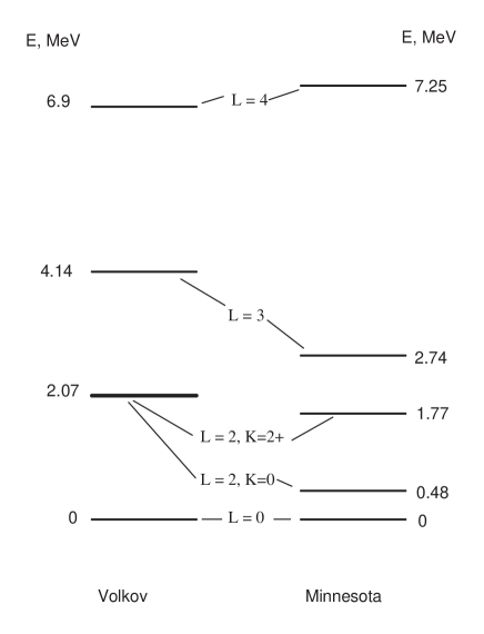
Figure 1: Spectrum of ¹⁰Be for the Hamiltonian (20) with Volkov and Minnesota interactions.

While the Volkov potential is consistent with the observed value for the radius of ¹⁰Be, the Minnesota potential with $u=0.98$ (this value of the exchange mixture parameter seems to be the best choice for the nuclei in the first half of the $p$-shell) leads to $r_{0}$=1.43 fm, and besides, yields a wrong sequence of excited states. The saturation is not reached for both potentials but, again, this is more evident in the Minnesota case (light nuclei being considered). Nevertheless, if $r_{0}$ is set to $1.64$ fm in the Minnesota case, one obtains the spectrum shown in Fig. 1 on the right. Now the $2^{+}$ states split as $V_{31}\neq V_{13}$. However, the splitting is just 1.29 MeV, which is twice smaller than observed (2.59 MeV). The splitting $E_{2}^{2}-E_{2}^{1}$ is proportional to $V_{31}-V_{13}$. Therefore, this value has to be increased in order to achieve a good description of the experimental results within the model. This suggestion is also supported by the fact that the value

$${1\over 2}(E_{2}^{2}+E_{2}^{1})-E_{0}=1.125\,\mbox{MeV}$$

appears to be four times less than the experimental one, and almost twice less than in the Volkov potential case ($2.07$ MeV).

Historically, both potentials were designed to describe the experimental data for the nuclei in the beginning of the $p$-shell. It is therefore not surprising that the their application to heavier nuclei may be accompanied by some corrections in the potentials themselves.

The Elliott’s scheme predicts the existence of the levels $3^{+}$ and $4^{+}$. Energy of the former is close to the sum of the energies of the $2^{+}$ states. The wave function of the latter has predominantly $K=4$ which affects the probabilities of E2 transitions. The isoscalar electric transition from the $4^{+}$ state to the $L=2,~{}K=0$ state is forbidden, leaving allowed only the transition to the $L=2,~{}K=2$ state.

It is important that a right choice of the central nucleon-nucleon interaction makes the states $L=2,K=0$ and $L=2,K=2$ uncoupled.

4 Effective Hamiltonian of the SU(3) model

When the overlap integral (20) was calculated, the operator $\hat{H}$ was acting on the generating Slater determinant $\Psi$. Its SU(3) symmetry was (2,2), and the result was projected to the states with the same symmetry. The projection was performed by an integration. Therefore, the overlap integral (20) keeps us within the basis of the representation $(2,2)$. In order to understand how the Hamiltonian $\hat{H}$ acts in this representation, we define an operator $\hat{H}({\bf u,w})$ as follows,

$$\langle\Psi|\hat{H}|\Psi\rangle=\hat{H}({\bf u,w})\langle\Psi|\Psi\rangle.$$ (27)

All operators which acting onto the basis states of an irreducible representations produce only those states which belong to the same representation are known: they are the group generators. We are interested here only in those expressions constructed from the SU(3) generators which are scalars with respect to the O(3) group. They are known, too [17], [18]. They are the operator ${\bf QQ}$ introduced by Elliott, and the operators $\hat{\Omega}={\bf LQL}$ and $\hat{\Omega}_{1}={\bf LQQL}$ [12]. All other operators may be written as polynomials of these three.

In our model the wave functions are represented by superpositions of the $D$-functions. Therefore, as in the case of the Hamiltonian of the triaxial rotator, all operators may be expressed via the SU(3) symmetry indices $\lambda,\mu$ and the three projections of the orbital momentum $L$ to the internal axes: $\hat{L}_{1},\hat{L}_{2},\hat{L}_{3}$. It has been shown[19] that

$$-\hat{\Omega}=a\hat{L}^{2}_{1}+b\hat{L}^{2}_{2}+c\hat{L}^{2}_{3}+\hat{\Omega}_{2},$$ (28)

$$-\hat{\Omega}_{1}=a^{2}\hat{L}^{2}_{1}+b^{2}\hat{L}^{2}_{2}+c^{2}\hat{L}^{2}_{3}-{2\over 3}\hat{\bf L}^{2}-\hat{L}^{2}_{2}+{1\over 2}(\hat{L}^{2}_{1}\hat{L}^{2}_{3}+\hat{L}^{2}_{3}\hat{L}^{2}_{1})+2b\hat{\Omega}_{2},$$ (29)

where

$$a={2\lambda+\mu+3\over 3},~{}~{}b={-\lambda+\mu\over 3},~{}~{}c={-\lambda-2\mu-3\over 3}.$$ (30)

$$\hat{\Omega}_{2}={i\over 6}\left(\hat{L}_{1}\hat{L}_{2}\hat{L}_{3}+\hat{L}_{2}\hat{L}_{3}\hat{L}_{1}+\hat{L}_{3}\hat{L}_{1}\hat{L}_{2}+\hat{L}_{2}\hat{L}_{1}\hat{L}_{3}+\hat{L}_{3}\hat{L}_{2}\hat{L}_{1}+\hat{L}_{1}\hat{L}_{3}\hat{L}_{2}\right).$$ (31)

The structure of the operators $\hat{\Omega}$ and $\hat{\Omega}_{1}$ is similar to that of the Hamiltonian of the triaxial rotator, but the inertial parameters (the coefficients of $\hat{L}^{2}_{1},~{}\hat{L}^{2}_{2},~{}\hat{L}^{2}_{3}$) are not the principle values of the tensor of inertia, but rather the principle values of the tensor of the intrinsic quadrupole momentum (in the case of $\hat{\Omega}$) or their squared values (in the case of $\hat{\Omega}_{1}$). Additional terms

$$\hat{\Omega}_{2}~{}~{}\mbox{and}~{}~{}{1\over 2}(\hat{L}^{2}_{1}\hat{L}^{2}_{3}+\hat{L}^{2}_{3}\hat{L}^{2}_{1})$$

only lead to the finite number of basis functions of an SU(3) representation whereas in the triaxial rotator case the basis is infinite.

The operators $\hat{\Omega}$ and $\hat{\Omega}_{1}$ commute with $\hat{\bf L}^{2}$, therefore the orbital momentum $L$, as expected, is a constant of motion. Besides, these operators are D₂-invariant, so that their eigenfunctions have a definite D₂ symmetry. However, among all eigenfunctions of $\hat{\Omega}$ and $\hat{\Omega}_{1}$, only those are of physical interest which have a D₂ symmetry identical to that of the basis states produced by the overlap integral (7).

It is natural to seek the eigenfunctions $\phi_{L,m}$ of $\hat{\Omega}$ (or $\hat{\Omega}_{1}$, or a linear combination of $\hat{\Omega}$ and $\hat{\Omega}_{1}$) in the form of a superposition of the functions

$$\sqrt{w_{L}^{\alpha}}\psi^{\alpha}_{L,m},$$

taking into account their normalization, that is

$$\phi_{L,m}=\sum_{\alpha}B_{L,\alpha}\sqrt{w_{L}^{\alpha}}\psi^{\alpha}_{L,m}.$$ (32)

Then the coefficients $B_{L,\alpha}$ must satisfy the following set of equations,

$$\sum_{\alpha^{\prime}}(\langle L,\alpha|\hat{\Omega}|L,\alpha^{\prime}\rangle-\delta_{\alpha,\alpha^{\prime}})B_{L,\alpha^{\prime}}=0.$$ (33)

One may calculate the matrix elements $\langle L,\alpha|\hat{\Omega}|L,\alpha^{\prime}\rangle$, by calculating first the matrix element of $\hat{\Omega}$ between the generating functions and then expanding the result,

$$\langle\Psi|\hat{\Omega}|\Psi\rangle=\sum_{L}\sum_{\alpha,\alpha^{\prime}}\sqrt{w^{\alpha}_{L}(\lambda,\mu)w^{\alpha^{\prime}}_{L}(\lambda,\mu)}\langle L,\alpha|\hat{\Omega}|L,\alpha^{\prime}\rangle\sum_{m}\psi^{\alpha}_{Lm}\tilde{\psi}^{\alpha^{\prime}}_{Lm}.$$ (34)

Alternatively, a simple formula (28) for $\hat{\Omega}$ provides for another way,

$$\hat{\Omega}\sqrt{w_{L}^{\alpha}}\psi^{\alpha}_{L,m}=\sum_{\alpha^{\prime}}\langle L,\alpha|\hat{\Omega}|L,\alpha^{\prime}\rangle\sqrt{w_{L}^{\alpha^{\prime}}}\psi^{\alpha}_{L,m}.$$ (35)

The action of the operators $\hat{L}_{1},\hat{L}_{2},\hat{L}_{3}$ on the $D$-functions is known (cf. [15]). Both approaches lead to the same Hermitian matrix,

$$||\langle L,\alpha|\hat{\Omega}|L,\alpha^{\prime}\rangle||.$$

Diagonalization of this matrix yields the eigenvalues of $\Omega$. At a given $L$, the size of the matrix depends on the number of possible values of $\alpha$.

Finally, one more possibility is to expand $\phi_{L,m}$ over the $D$-functions straightforwardly,

$$\phi_{L,m}=N_{L}\sum_{K}A_{L,K}D^{L}_{K\pm,m}.$$ (36)

This way is the simplest, it results in a non-Hermitian matrix

$$||\langle L,K\pm|\hat{\Omega}|L,K^{\prime}\pm\rangle||,$$ (37)

because $\hat{\Omega}_{2}$ (a term in both $\hat{\Omega}$ and $\hat{\Omega}_{1}$) contains an imaginary unit $i$ as a factor, and that makes it a non-self-conjugate operator. This does not mean, however, that the matrix will necessarily have complex eigenvalues . The coefficients $A_{L,K}$ are found from the set

$$\sum_{K^{\prime}}(\langle L,K\pm|\hat{\Omega}|L,K^{\prime}\pm\rangle-\delta_{K,K^{\prime}})A_{L,K}=0,$$ (38)

where the matrix elements $\langle L,K\pm|\hat{\Omega}|L,K^{\prime}\pm\rangle$ are defined by

$$\hat{\Omega}D^{L}_{K\pm,m}=\sum_{K^{\prime}}\langle L,K\pm|\hat{\Omega}|L,K^{\prime}\pm\rangle D^{L}_{K^{\prime}\pm,m}.$$ (39)

The normalization factor $N_{L}$ of the eigenvalues (36) is found from the condition

$$N_{L}\sum_{\alpha}{1\over\sqrt{w_{L}^{\alpha}}}\sum_{K}A_{L,K}C^{\alpha}_{L,K}=1.$$ (40)

The coefficients $C^{\alpha}_{L,K}$ were defined above ((11) and (12)). They can be found by expanding the overlap integral (7) over the basis states of an irreducible representation of the SU(3) group. The summation over $K$ in (40) signifies the projection of an eigenfunction of $\hat{\Omega}$ to the allowed states. Hence those eigenfunctions of $\hat{\Omega}$ for which each of the sums

$$\sum_{K}A_{L,K}C^{\alpha}_{L,K}$$

vanishes are forbidden. They do not satisfy the Pauli exclusion principle and must be disregarded. With $L$ increasing, such states appear, sooner or later, and this must be taken into account in the calculations of spectra.

5 General remarks on the effective Hamiltonian

At least at the first stage, the effective Hamiltonian is better to be constructed as a linear combination of the operators ${\bf QQ}$, $\hat{\Omega}$ and $\hat{\Omega}_{1}$. It is now clear that the result will be, in fact, the Hamiltonian of the triaxial rotator model with some additional terms which may be important in the actual calculations of the LR spectra. The coefficients of the three operators may then serve as phenomenological parameters.

The question is, can such a Hamiltonian describe the observed low-energy spectra of even-even nuclei? One may believe that the phenomenological parameters would be the same for a whole range of nuclei while the SU(3) symmetry indices would change from nucleus to nucleus according to known general rules.

Such an approach has been used in [17] and [18], and there an attempt was made to extend the model to excited states with higher $L$. Then, one may question, whether it suffices to have the three operators entering the Hamiltonian in their first order, or a higher-order terms are necessary?

In Ref. [20] the authors studied the ²⁰Ne and ⁴⁴Ti nuclei and concluded, that the effective Hamiltonian of their LR $(\lambda,0)$ ((8,0) for ²⁰Ne and (12,0) for ⁴⁴Ti), derived from the overlap integrals of the generating Slater determinants with the Gaussian interaction, contains first two orders of ${\bf QQ}$ for ²⁰Ne, and first three orders for ⁴⁴Ti. It became clear that higher orders are necessary for higher oscillator shells. The influence of higher-order terms is increasing with $L$. For representations $(\lambda,0)$, the operators $\hat{\Omega}$ and $\hat{\Omega}_{1}$ degenerate and reduce to the operator $\hat{\bf L}^{2}$. Hence to derive the terms containing high orders of $\hat{\Omega}$ and $\hat{\Omega}_{1}$, one has to use the LRs with $\lambda\neq 0,\mu\neq 0$ and go beyond the $p$-shell. Alternatively, the higher-order terms may be included in the Hamiltonian phenomenologically.

6 The mass quadrupole operator

We now show that $a,~{}b,~{}c$ are the principle values of the quadrupole momentum. To start with, the explicit form of the operator of the mass quadrupole momentum $\hat{Q}_{\alpha\beta}$ in the intrinsic coordinate frame is shown in [19]. The same operator in the laboratory frame (with our choice of axes) is

$$\hat{Q}_{2m}={1\over 3}(-\lambda+\mu)D^{2}_{m,0}+{\sqrt{3}\over 3}(\lambda+\mu)D^{2}_{m,2+}-{\sqrt{3}\over 3}\left(D^{2}_{m,1+}\hat{L}_{1}+iD^{2}_{m,1-}\hat{L}_{3}+D^{2}_{m,2-}\hat{L}_{2}\right).$$ (41)

Here

$${1\over 3}(-\lambda+\mu)~{}~{}\mbox{and}~{}~{}{\sqrt{3}\over 3}(\lambda+\mu)$$

are the principle values of the traceless tensor of the quadrupole momentum.

It follows from (41) that

$${\bf QQ}={2\over 3}(\lambda^{2}+\lambda\mu+\mu^{2}+3\lambda+3\mu)-{1\over 2}\hat{\bf L}^{2}.$$ (42)

Also note that

$$-{\sqrt{3}\over 3}\left(D^{2}_{m,1+}\hat{L}_{1}+iD^{2}_{m,1-}\hat{L}_{3}+D^{2}_{m,2-}\hat{L}_{2}\right)D^{2}_{m^{\prime},2+}=$$

$$=-{\sqrt{3}\over 3}\left(D^{2}_{m,1+}D^{2}_{m^{\prime},1+}-D^{2}_{m,1-}D^{2}_{m^{\prime},1-}+2D^{2}_{m,2-}D^{2}_{m^{\prime},2-}\right).$$ (43)

We have arrived to an expected, D₂-invariant expression. Indeed, acting on such an expression, the operator of the quadrupole momentum must yield another D₂-invariant expression.

Consider now the Eliiott’s choice of axes.

$$\hat{Q}_{2m}={2\over 3}\left\{(\bar{a}-{\bar{b}+\bar{c}\over 2})D^{2}_{m,0}+{\sqrt{3}\over 2}(\bar{b}-\bar{c})D^{2}_{m,2+}\right\}+...={1\over 3}(2\lambda+\mu)D^{2}_{m,0}+{\sqrt{3}\over 3}\mu D^{2}_{m,2+}+...$$

By definition,

$$\bar{a}={1\over 3}(2\lambda+\mu)=a-1,~{}~{}\bar{b}={1\over 3}(-\lambda+\mu)=b,~{}~{}\bar{c}={1\over 3}(-\lambda-2\mu)=c+1.$$

Then, for the representation $(\lambda,0)$ one obtains

$$\hat{Q}_{2m}={2\lambda\over 3}D^{2}_{m,0}+...$$ (44)

In this case, the axially symmetric nucleus has a prolate shape and therefore its intrinsic quadrupole momentum is directed along the rotation axis and is positive.

Yet another choice,

$$\hat{Q}_{2m}={2\over 3}\left\{(\bar{c}-{\bar{a}+\bar{b}\over 2})D^{2}_{m,0}+{\sqrt{3}\over 2}(\bar{a}-\bar{b})D^{2}_{m,2+}\right\}+...=$$

$$=-{1\over 3}(2\mu+\lambda)D^{2}_{m,0}+{\sqrt{3}\over 3}\lambda D^{2}_{m,2+}+...$$

is convenient for the limiting case of $(0,\mu)$, when

$$\hat{Q}_{2m}=-{2\mu\over 3}D^{2}_{m,0}+...$$ (45)

Now the nucleus has an oblate shape, the quadrupole momentum is again oriented along the rotation axis but this time, negative.

Finally, we show the matrix elements of the isoscalar E1 transition from the ground state to the states $\psi^{\alpha}_{2,m}$ of the Elliott’s basis when the indices $\lambda,\mu$ are both even.

$$\langle L=2,\alpha=1,m|\hat{Q}_{2m}|L=0\rangle=\sqrt{{w_{0}\over w^{1}_{2}}}\left\{{1\over 3}(-\lambda+\mu)C^{1}_{20}+{\sqrt{3}\over 3}(\lambda+\mu)C^{1}_{22}\right\},$$ (46)

$$\langle L=2,\alpha=2,m|\hat{Q}_{2m}|L=0\rangle=\sqrt{{w_{0}\over w^{2}_{2}}}\left\{{1\over 3}(-\lambda+\mu)C^{2}_{20}+{\sqrt{3}\over 3}(\lambda+\mu)C^{2}_{22}\right\}.$$ (47)

7 Effective Hamiltonian for ¹⁰Be

We shall now try to built an effective Hamiltonian for ¹⁰Be from ${\bf L}^{2},~{}\hat{\Omega},~{}\hat{\Omega}_{1}$. The only condition we impose on the Hamiltonian is the equivalence of its spectra (eigenvalues and eigenvectors) to that found above in the LR approximation.

$$\hat{H}({\bf u,w})=B\left({3\over 2}-{1\over 8}~{}{\bf L}^{2}\right)+\left(A-{B\over 4}\right)\left(p+q{\bf L}^{2}+r\hat{\Omega}_{1}+s\hat{\Omega}\right),$$ (48)

where $p,q,r,s$ are the coefficients to be found.

We have noted earlier that the matrix elements of the norm and Hamiltonian operators between the basis functions $\psi_{2m}^{1}$ and $\psi_{2m}^{2}$ with $L=2$ are diagonal only. Meanwhile, the eigenfunctions of $\hat{\Omega}$ are linear combinations of these states. Therefore, $s=0$, and it is the operator $\hat{\Omega}_{1}$ that splits the two levels with $L=2$. It follows (23) and (24), that

$$E^{2}_{2}-E_{2}^{1}={8\over 5}~{}\left(A-{B\over 4}\right).$$ (49)

The eigenvalues of $\hat{\Omega}_{1}$ in these states are

$$\hat{\Omega}_{1}\psi_{2m}^{1}=-44~{}\psi_{2m}^{1},~{}~{}\hat{\Omega}_{1}\psi_{2m}^{2}=-12~{}\psi_{2m}^{2}.$$ (50)

Using

$$E_{0}=5A+{1\over 4}B,~{}\mbox{and}~{}E^{1}_{2}-E_{0}=-{18\over 5}\left(A-{B\over 4}\right)-{3\over 4}B,$$ (51)

we define $p,q,r$ and obtain the effective Hamiltonian in its final form,

$$\hat{H}({\bf u,w})=B\left({3\over 2}-{1\over 8}~{}{\bf L}^{2}\right)+\left(A-{B\over 4}\right)\left(5-{7\over 30}~{}{\bf L}^{2}+{1\over 20}~{}\hat{\Omega}_{1}\right).$$ (52)

One may check straightforwardly that this Hamiltonian yields the same values of $E_{3}$ and $E_{4}$, too.

In the phenomenological approach, the coefficients $A$ and $B$ should be chosen so that to reproduce the experimental spectrum of ¹⁰Be. It would suffice then to use the energy of the first three states, $E_{0},E_{2}^{1}$ and $E_{2}^{2}$. The energies $E_{3}$ and $E_{4}$ could serve as a test. But their experimental values are not known at present.

8 Summary

We have shown that the realization of the SU(3) LR approximation with the microscopic Hamiltonian and a nucleon-nucleon potential (such as the Volkov and Minnesota potentials) may be reduced to the calculations with an effective potential. The latter is a linear combination of the operators $\hat{\bf L}^{2}$, $\hat{\Omega}$ and $\hat{\Omega}_{1}$, as well as their higher orders. In many ways this Hamiltonian is similar to that of the triaxial rotator model. However, the inertial parameters of such a rotator are not inversely proportional to the principal values of the tensor of inertia, but proportional to the principal values of the tensor of the quadrupole momentum. Both the basis functions of an irreducible representation of the SU(3) group and the basis functions of the rotator model are superpositions of Wigner’s $D$-functions, but their normalization should be calculated separately.

Some problems appearing in the calculations of the spectra of nuclei in the second half of the $p$-shell with the Volkov and Minnesota potentials are discussed.

Some remarks on the structure of effective Hamiltonians of medium and heavy nuclei are also given.

References

- [1] J. P. Elliott, Proc. Roy. Soc. London, A 245 (1958), 128; A 245 (1958), 562.
- [2] A. Arima, M. Harvey, K. Shimizu, Phys. Lett. B 30 (1969), 517.
- [3] K. T. Hecht, A. Adler. Nucl. Phys, A137 (1969), 129.
- [4] R. D. Ratna Raji, J. P. Draayer, K. T. Hecht, Nucl. Phys. A202 (1973), 433.
- [5] N. Lo Iudice, F. Palumbo, Phys. Rev. Lett. 41 (1978), 1532.
- [6] T. Beushel, J. P. Draayer, D. Rompf, J. G. Hirsch. Phys. Rev. C57 (1998), 1233.
- [7] J. G. Hirsch, P. O. Hess, L. Hernandez, C. Vargas, T. Beushel, J. P. Draayer, Rev. Mex. Fis. 45 Supl. 2 (1999), 86.
- [8] D. Rompf, T. Beushel, J. P. Draayer, W. Scheid, J. G. Hirsch, Phys. Rev. C57 (1998), 1703.
- [9] A. B. Volkov, Nucl. Phys. 74 (1965), 33.
- [10] D. R. Thompson, M. LeMere, Y. C. Tang. Nucl. Phys. A286 (1977), 53.
- [11] A. S. Davydov, G. F. Filippov, Nucl. Phys. 8 (1958), 237.
- [12] V. Bargmann and M. Moshinsky. Nucl. Phys. 18 (1960), 4.
- [13] R. E. Peierls and J. Yoccoz. Proc. Phys. Soc. 70 (1957), 381.
- [14] A. S. Davydov, Quantum Mechanics, Pergamon Press, 1976.
- [15] L. D. Landau and E. M. Lifshitz, Quantum Mechanics: Non-Relativistic Theory, Pergamon Press, 1965.
- [16] I. Tanihata, T. Kobayashi, O. Yamakawa, S. Shimoura, K. Ekuni, K. Sugimoto, N. Takahashi, T. Shimoda, H. Sato, Phys. Lett. B 206 (1988), 592.
- [17] J. P. Draayer, K. J. Weeks, Phys. Rev. Lett. 51 (1983), 1422.
- [18] J. P. Draayer, K. J. Weeks, Ann. Phys. (New York) 156 (1984), 41.
- [19] G. F. Filippov, J. P. Draayer. Phys. Part. Nucl. 29 (1998), 548.
- [20] I. P. Okhrimenko, A. I. Steshenko, Preprint ITF-82-96R, Kiev, 1982 (in Russian).