Final state interaction contribution to the response of confined relativistic particles

Abstract

We report studies of the response of a massless particle confined by a potential. At large momentum transfer $\mathbf{q}$ it exhibits $\tilde{y}$ or equivalently Nachtmann $\xi$ scaling, and acquires a constant width independent of $\mathbf{q}$. This width has a contribution from the final state interactions of the struck particle, which persists in the $|\mathbf{q}|\rightarrow\infty$ limit. The width of the response predicted using plane wave impulse approximation is smaller because of the neglect of final state interactions in that approximation. However, the exact response may be obtained by folding the approximate response with a function representing final state interaction effects. We also study the response obtained from the momentum distribution assuming that the particle is on the energy shell both before and after being struck. Quantitative results are presented for the special case of a linear confining potential. In this case the response predicted with the on-shell approximation has correct values for the total strength, mean energy and width, however its shape is wrong.

I Introduction

Scattering of high energy probes from composite systems, such as electron scattering by nuclei Frois and Sick (1991) and nucleons Ellis et al. (1996), or neutron scattering by liquid helium Silver and Sokol (1989), is often used to study the structure of the bound system. The common assumption is that in deep inelastic scattering (DIS) at sufficiently high energy the probe is incoherently scattered by the constituents of the system. In the plane wave impulse approximation (PWIA), which neglects final state interaction (FSI) effects, DIS is directly related to the momentum and energy distribution of the constituents in the target.

The role of FSI effects has been studied extensively in electron scattering from nuclear targets Benhar et al. (1991); Benhar and Pandharipande (1993) and neutron scattering from liquid helium Silver and Sokol (1989). Recently it has been suggested that they may also influence DIS of leptons by hadrons Brodsky et al. (2001). In the present study we focus on scattering from targets with confined constituents. The corresponding physical case concerns DIS from nucleons where, in distinction from the nuclear and liquid helium cases, the constituents are confined in both the initial and final states.

We Paris and Pandharipande (2001) have recently studied the response of a massless particle confined by a linear (flux-tube) potential using the simple model Hamiltonian

$$H=\sqrt{|{\mathbf{p}}|^{2}}+\sqrt{\sigma}r,$$ (1)

to gain insights into DIS of leptons by hadrons. The response to a hypothetical scalar probe is calculated as a function of the momentum and energy transfer, $\mathbf{q}$, $\nu$ in the lab frame. It is given by

$$R(\mathbf{q},\nu)=\sum_{I}|\langle I|e^{i\mathbf{q}\cdot\mathbf{r}}|0\rangle|^{2}\delta(E_{I}-E_{0}-\nu),$$ (2)

where the sum is over all energy eigenstates $I$. The natural scaling variable in the many-body theory approach to DIS is $\tilde{y}=\nu-|\mathbf{q}|$ Benhar et al. (2000). In the large $|\mathbf{q}|$ or scaling limit the response depends only on $\tilde{y}$, not on $|\mathbf{q}|$ and $\nu$ independently. This scaling of the response is equivalent to the Nachtmann scaling, since the Nachtmann Nachtmann (1973) scaling variable $\xi=-\tilde{y}/M$, where $M$ is the hadron mass. In Ref. Paris and Pandharipande (2001) the $R(\mathbf{q},\nu)$ is calculated for $|\mathbf{q}|\leq 10$ GeV for the typical value of the string tension $\sqrt{\sigma}=1$ GeV/fm in QCD, by calculating all the relevant states $|I\rangle$ contributing to the response.

In this work we study the effects of the FSI of the struck particle on the response; analytic calculations of the width of the response are presented in Sec.II, and the numerical results for a linear confining potential are given in Sec.III. Both indicate that the FSI increase the width of the response beyond that predicted by PWIA. The analytic calculations also consider the nonrelativistic problem, in which $\mathbf{q}$ is large compared to all the momenta in the target, but smaller than the constituent mass $m$. The main differences between the nonrelativistic and the relativistic response are that the former peaks at $\nu=|\mathbf{q}|^{2}/2m$ and has a width proportional to $|\mathbf{q}|$, while the latter peaks at $\nu\sim|\mathbf{q}|$, and has a constant width in the scaling limit. The folding function Benhar (1999) representing the effects of the FSI on the response is discussed in the last section, Sec.IV, where conclusions are given.

II Moments of the Response

In the case of a single confined particle, the state of the system after the probe has struck the target is

$$|X\rangle=e^{i\mathbf{q}\cdot\mathbf{r}}|0\rangle,$$ (3)

where $|0\rangle$ denotes the ground state of the particle. The state $|X\rangle$ is not an eigenstate of the Hamiltonian and therefore has a distribution in energy. It has a unit norm, $\langle X|X\rangle=\langle 0|e^{-i\mathbf{q}\cdot\mathbf{r}}e^{i\mathbf{q}\cdot\mathbf{r}}|0\rangle=1$. The total strength of the response, given by the static structure function

$$S(|\mathbf{q}|)=\int_{0}^{\infty}d\nu\,R(|\mathbf{q}|,\nu),$$ (4)

is therefore unity. In many-body systems $S(|\mathbf{q}|)$ is not necessarily equal to one. Subsequent formulas pertain to the general case and show factors of $S(|\mathbf{q}|)$ explicitly.

The mean excitation energy of the state $|X\rangle$ is given by the first moment of the response:

$$\overline{\nu}(|\mathbf{q}|)=\frac{1}{S(|\mathbf{q}|)}\langle X|H-E_{0}|X\rangle=\frac{1}{S(|\mathbf{q}|)}\int_{0}^{\infty}d\nu\,\nu\,R(|\mathbf{q}|,\nu).$$ (5)

The width of the distribution in energy is characterized by the second moment of the energy about the mean:

$$\Delta^{2}(|\mathbf{q}|)=\frac{1}{S(|\mathbf{q}|)}\langle X|\left(H-\frac{\langle X|H|X\rangle}{S(|\mathbf{q}|)}\right)^{\!2}|X\rangle.$$ (6)

For example, if the response is Gaussian, it is completely determined by these three moments:

$$R_{G}(\mathbf{q},\nu)=\frac{S(|\mathbf{q}|)}{\sqrt{\pi\Delta^{2}(|\mathbf{q}|)}}e^{-(\nu-\overline{\nu}(|\mathbf{q}|))^{2}/\Delta^{2}(|\mathbf{q}|)}.$$ (7)

The full-width at half-maximum (FWHM) of a Gaussian response is given by $2\Delta(|\mathbf{q}|)\sqrt{\ln 2}\approx\frac{5}{3}\Delta(|\mathbf{q}|)$. Obviously many more moments are required to describe a response of more general shape. Nevertheless, a necessary condition for the occurrence of the $\tilde{y}$ or Nachtmann $\xi$ scaling is that $S(|\mathbf{q}|)$, $\overline{\nu}(|\mathbf{q}|)-|\mathbf{q}|$, $\Delta(|\mathbf{q}|)$, and all the higher moments become independent of $|\mathbf{q}|$, since the response depends only on $\nu-|\mathbf{q}|$ when $|\mathbf{q}|\rightarrow\infty$.

In the remainder of this section we will calculate the average excitation energy, $\overline{\nu}(|\mathbf{q}|)$ and the width, $\Delta(|\mathbf{q}|)$ for the model Hamiltonian of Eq.(1) in the scaling limit, $|\mathbf{q}|\rightarrow\infty$. They are calculated analytically for a general potential $V(r)$. Section III presents numerical results for the case of a linear confining potential. This analysis allows the comparison of the results for the exact response with the following two common approximations. The PWIA, which assumes that the final state of the struck particle can be approximated by a plane wave in an average potential, is commonly used in nuclear physics. And the on-shell approximation (OSA), in which the struck particle is assumed to be in a plane wave state with the energy of that of a free particle, before and after the interaction with the probe, used in hadron physics.

We proceed with the evaluation of the average excitation energy [Eq.(5)] for the case of the exact response. The kinetic energy term of the matrix element $\langle X|H|X\rangle$ is

$$\langle X|\sqrt{|\mathbf{p}|^{2}}|X\rangle=\int\frac{d^{3}k}{(2\pi)^{3}}n(k)|\mathbf{k}+\mathbf{q}|,$$ (8)

where we have transformed to momentum space and $n(k)=|\psi_{0}(k)|^{2}$. In the scaling limit, with $\mathbf{q}=|\mathbf{q}|\hat{\mathbf{z}}$, we can expand $|\mathbf{q}+\mathbf{k}|$ and obtain:

$$|\mathbf{k}+\mathbf{q}|=|\mathbf{q}|+k_{z}+\frac{1}{2|\mathbf{q}|}k^{2}_{\perp}-\frac{1}{2|\mathbf{q}|^{2}}k^{2}_{\perp}k_{z}+\mathcal{O}\left(\frac{1}{|\mathbf{q}|^{3}}\right).$$ (9)

Here $\mathcal{O}\left(\frac{1}{|\mathbf{q}|^{3}}\right)$ denotes the neglected terms of that and higher order, and $k^{2}_{\perp}=k^{2}_{x}+k^{2}_{y}$. Substituting this expansion into Eq.(5) yields,

$$\overline{\nu}(|\mathbf{q}|)=|\mathbf{q}|+\langle V\rangle_{0}-E_{0}+\frac{1}{3|\mathbf{q}|}\langle k^{2}\rangle_{0}+\mathcal{O}\left(\frac{1}{|\mathbf{q}|^{3}}\right);$$ (10)

the term of $\mathcal{O}\left(\frac{1}{|\mathbf{q}|^{2}}\right)$ is zero by symmetry. Note that $E_{0}-\langle V\rangle_{0}=\langle T\rangle_{0}$, where $T$ denotes the kinetic energy. Thus $\overline{\nu}(|\mathbf{q}|)=|\mathbf{q}|-\langle T\rangle_{0}$ in the limit $|\mathbf{q}|\rightarrow\infty$. The requirement that $\overline{\nu}(|\mathbf{q}|)-|\mathbf{q}|$ becomes constant is naturally satisfied in this limit.

The width [Eq.(6)] depends on the matrix element $\langle X|H^{2}|X\rangle$; $H^{2}=p^{2}+\sqrt{p^{2}}V(r)+V(r)\sqrt{p^{2}}+V^{2}(r)$. The first term of $H^{2}$ gives:

$$\langle X|p^{2}|X\rangle=\langle|\mathbf{k}+\mathbf{q}|^{2}\rangle_{0}=|\mathbf{q}|^{2}+\langle k^{2}\rangle_{0}\ .$$ (11)

The average of the second and third terms in $H^{2}$ may be shown to be equal to each other and

$$\langle X|\sqrt{p^{2}}V|X\rangle = \int\frac{d^{3}k}{(2\pi)^{3}}\psi_{0}^{*}(k)|\mathbf{q}+\mathbf{k}|[V\psi_{0}](k)$$ (12)

$$\approx |\mathbf{q}|\langle V\rangle_{0}+\frac{1}{2|\mathbf{q}|}\langle k^{2}_{\perp}V\rangle_{0}+\mathcal{O}\left(\frac{1}{|\mathbf{q}|^{3}}\right),$$

where $[V\psi_{0}](k)=\int d^{3}re^{i\mathbf{k}\cdot\mathbf{r}}V(r)\psi_{0}(r)$. Substitution into Eq.(6) with $S(|\mathbf{q}|)=1$ gives:

$$\Delta^{2}(|\mathbf{q}|)=\frac{1}{3}\langle k^{2}\rangle_{0}+\langle V^{2}\rangle_{0}-\langle V\rangle_{0}^{2}+\frac{2}{3|\mathbf{q}|}\left(\langle k^{2}V\rangle_{0}-\langle k^{2}\rangle_{0}\langle V\rangle_{0}\right)+\mathcal{O}\left(\frac{1}{|\mathbf{q}|^{2}}\right).$$ (13)

This expression demonstrates that the width of the exact response is independent of $|\mathbf{q}|$ in the limit $|\mathbf{q}|\rightarrow\infty$ as necessary for $\tilde{y}$ scaling. It also shows that the width has a kinematic contribution dependent upon the target momentum distribution, and an additional interaction contribution.

As mentioned, the PWIA assumes that a constituent of momentum $\mathbf{k}$, after being struck by the probe, may be described by a plane wave with momentum $\mathbf{k+q}$ in an assumed average potential chosen to give the exact $\overline{\nu}$ of Eq.(10). The PWIA response is

$$R_{PWIA}(|\mathbf{q}|,\nu)=\int\frac{d^{3}k}{(2\pi)^{3}}n(k)\delta(e(\mathbf{k}+\mathbf{q})-E_{0}-\nu)$$ (14)

where $e(\mathbf{k}+\mathbf{q})$ is the energy of the plane wave, taken to be:

$$e(\mathbf{k}+\mathbf{q})=|\mathbf{k}+\mathbf{q}|+\langle V\rangle_{0}.$$ (15)

The first term is the kinetic energy of the struck particle. The second term is the average of the potential in the final state of the system given by, $\langle X|V|X\rangle=\langle 0|e^{-i\mathbf{q}\cdot\mathbf{r}}Ve^{i\mathbf{q}\cdot\mathbf{r}}|0\rangle=\langle V\rangle_{0}$. The $R_{PWIA}(|\mathbf{q}|,\nu)$ exhibits $\tilde{y}$ scaling as can be easily seen by expanding the argument of the $\delta$ function in $R_{PWIA}$. In the large $|\mathbf{q}|$ limit $R_{PWIA}$ depends only on $\tilde{y}=\nu-|\mathbf{q}|$.

The average energy and the width of the PWIA response are calculated using:

$$\int_{0}^{\infty}d\nu\,\nu^{n}R_{PWIA}(|\mathbf{q}|,\nu)=\int_{0}^{\infty}d\nu\,\nu^{n}\int\frac{d^{3}k}{(2\pi)^{3}}n(k)\delta(e(\mathbf{k}+\mathbf{q})-E_{0}-\nu).$$ (16)

The average excitation energy, obtained with $n=1$, agrees with the exact result in Eq.(10) by construction.

The width of the PWIA response, however, is not the same as the width of the exact response.

$$\Delta^{2}_{PWIA}=\frac{1}{3}\langle k^{2}\rangle_{0}+\mathcal{O}\left(\frac{1}{|\mathbf{q}|^{2}}\right)$$ (17)

contains only the first term of the exact result [Eq.(13)] due to the target momentum distribution. The second term, $\langle V^{2}\rangle_{0}-\langle V\rangle_{0}^{2}$, of the exact $\Delta^{2}$ represents the FSI contribution neglected in the PWIA. It does not vanish in the $|\mathbf{q}|\rightarrow\infty$ limit for relativistic kinematics.

In the non-relativistic case, $H_{NR}=\frac{|\mathbf{p}|^{2}}{2m}+V(r)$, the exact $\overline{\nu}$ is given by:

$$\overline{\nu}_{NR}=\frac{1}{2m}|\mathbf{q}|^{2}\ .$$ (18)

The nonrelativistic-PWIA (NR-PWIA) response:

$$R_{NR-PWIA}(|\mathbf{q}|,\nu)=\int\frac{d^{3}k}{(2\pi)^{3}}n(k)\delta\left(\frac{|\mathbf{q}+\mathbf{k}|^{2}}{2m}+\langle V\rangle_{0}-E_{0}-\nu\right)$$ (19)

gives the exact $\overline{\nu}$. For the width of the NR-PWIA response we obtain:

$$\Delta^{2}_{NR-PWIA}(|\mathbf{q}|)=|\mathbf{q}|^{2}\frac{\langle k^{2}\rangle_{0}}{3m^{2}}+\frac{1}{4m^{2}}\left(\langle k^{4}\rangle_{0}-\langle k^{2}\rangle_{0}^{2}\right).$$ (20)

Note that in Eqs.(18) and (20) we have not taken the $|\mathbf{q}|\rightarrow\infty$ limit.

The width of the exact NR response is:

$$\Delta^{2}_{NR}(|\mathbf{q}|)=\Delta^{2}_{NR-PWIA}+\frac{1}{m}\left(\langle Vk^{2}\rangle_{0}-\langle V\rangle_{0}\langle k^{2}\rangle_{0}\right)+\langle V^{2}\rangle_{0}-\langle V\rangle_{0}^{2}\ .$$ (21)

It differs from $\Delta_{NR-PWIA}$ in terms of order $1/|\mathbf{q}|$ which can be neglected in the scaling limit. Thus, in contrast to the relativistic case, the FSI do not increase the width of the NR-PWIA response at large $|\mathbf{q}|$.

Finally we consider the on-shell approximation (OSA) in which the energy of the struck constituent is that of a free relativistic particle before and after the interaction with probe, as assumed in the quark-parton model. The response in OSA is

$$R_{OSA}(|\mathbf{q}|,\nu)=\int\frac{d^{3}k}{(2\pi)^{3}}n(k)\delta\left(|\mathbf{k}+\mathbf{q}|-|\mathbf{k}|-\nu\right);$$ (22)

it depends only on the momentum distribution of target constituents and obeys $\tilde{y}$ scaling. The average excitation in OSA is

$$\overline{\nu}_{OSA}=|\mathbf{q}|-\langle T\rangle_{0}+\frac{1}{3|\mathbf{q}|}\langle k^{2}\rangle_{0}+\mathcal{O}\left(\frac{1}{|\mathbf{q}|^{3}}\right),$$ (23)

and the width is given by:

$$\Delta^{2}_{OSA}=\frac{1}{3}\langle k^{2}\rangle_{0}+\langle k^{2}\rangle_{0}-\langle T\rangle_{0}^{2}+\mathcal{O}\left(\frac{1}{|\mathbf{q}|}\right).$$ (24)

The exact value of $\overline{\nu}$ [Eq.(10)] is reproduced by the OSA for any potential. However, the $\Delta^{2}_{OSA}$ has $\langle k^{2}\rangle_{0}-\langle T\rangle_{0}^{2}$ in place of the $\langle V^{2}\rangle_{0}-\langle V\rangle_{0}^{2}$ in the leading term of the exact $\Delta^{2}$ [Eq.(13)]. For a massless particle in a linear confining potential, i.e. for the Hamiltonian of Eq.(1), $\langle T\rangle_{0}=\langle V\rangle_{0}$, and $\langle k^{2}\rangle_{0}=\langle V^{2}\rangle_{0}$. Therefore for this particular Hamiltonian the OSA reproduces the exact value of $\Delta$.

The calculated responses shown in the next section however indicate that the shape of the OSA response is incorrect. We have calculated the third moment of the $H$ in the state $|X\rangle$ and observed that the exact and OSA responses indeed give different values. We expect the moments to differ also for orders higher than the third since the shapes of the exact and the OSA response are very different.

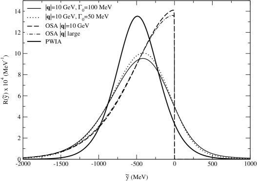
Figure 1: The response versus $\tilde{y}$ calculated exactly for $\Gamma_{0}=100$ MeV (thin solid curve) and $\Gamma_{0}=50$ MeV (dotted curve). The response in OSA are shown for $|\mathbf{q}|=10$ GeV (dashed) and $|\mathbf{q}|\rightarrow\infty$ (dot-dashed). The PWIA response for $|\mathbf{q}|=10$ GeV and $|\mathbf{q}|\rightarrow\infty$ lie on essentially the same (thick solid) curve.

III Numerical results

We first compare the response functions for $|\mathbf{q}|=10$ GeV before comparing their moments. In Ref. Paris and Pandharipande (2001) it has been shown that the scaling limit is obtained for such values of $|\mathbf{q}|$. The exact response, Eq.(2), is a sequence of $\delta$ functions at $\nu=E_{I}-E_{0}$. In order to obtain a smooth response we assume decay widths $\Gamma_{0}$ for all the excited states. Note that the energies of the states $|I\rangle$ that contribute to the response at $|\mathbf{q}|=10$ GeV are large, therefore their decay widths are not affected by the energy dependent terms assumed in Ref. Paris and Pandharipande (2001). The response including decay widths is given by:

$$R(\mathbf{q},\nu)=\sum_{I}|\langle I|e^{i\mathbf{q}\cdot\mathbf{r}}|0\rangle|^{2}\left(\frac{\Gamma_{0}}{2\pi}\right)\frac{1}{(E_{I}-E_{0}-\nu)^{2}+\Gamma_{0}^{2}/4}\ .$$ (25)

The responses obtained with $\Gamma_{0}=100$ and 50 MeV are shown in Fig. 1, along with the PWIA and OSA responses for $|\mathbf{q}|=10$ GeV and for $|\mathbf{q}|\rightarrow\infty$. The difference between the exact responses for $\Gamma_{0}=100$ and 50 MeV are much smaller than those between the exact and the approximate.

We note that the shape of the PWIA response is qualitatively similar to that of the exact, however, its width is too small. This is a direct consequence of the neglect of interaction terms in $\Delta$ [Eq.(13)] as discussed in the last section. The width $\Delta$ of the response for $\Gamma_{0}\rightarrow 0$, is 409 MeV, while the $\Delta_{PWIA}=326$ MeV. Note that for a Gaussian response, Eq.(7) the FWHM is $\sim 5\Delta/3$. The FWHM of the exact and the PWIA responses shown in Fig. 1 are larger because they are not exactly Gaussian.

The OSA results in the discontinuous curves shown in Fig. 1. They are discontinuous at the lightline ($|\mathbf{q}|=\nu$) because the response of free particles is limited to the spacelike region $\nu<|\mathbf{q}|$. The discontinuity at $\tilde{y}=0$ is in clear conflict with the exact response which is continuous across the lightline and is non-zero in the timelike ($\tilde{y}>0$) region. Therefore the OSA appears to be unsatisfactory even though for the special case of a linear potential it has the exact values of $S(|\mathbf{q}|)$, $\overline{\nu}(|\mathbf{q}|)$ and $\Delta(|\mathbf{q}|)$.

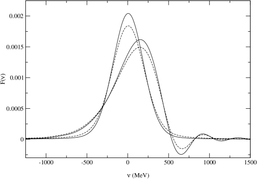
Figure 2: Folding functions for large $|\mathbf{q}|$. The solid and dashed curves correspond to $\Gamma_{0}=50$ and 100 MeV, respectively. The approximate folding functions $F_{A}$ of Eq.(29) are peaked at $\nu=0$ while the folding functions obtained from the exact and PWIA response by deconvolution are peaked at $\nu\sim 0.2$ GeV.

IV FSI Folding function

The exact response may be obtained from $R_{PWIA}(|\mathbf{q}|,\nu)$ via convolution with the folding function Silver and Sokol (1989); Benhar et al. (1991); Benhar (1999). The states $|\mathbf{k}+\mathbf{q}\rangle$ used in the PWIA are not eigenstates of the $H$. Therefore they must have a distribution in energy, and we may express the exact response as:

$$R(|\mathbf{q}|,\nu)=\int d\nu^{\prime}F(|\mathbf{q}|,\nu-\nu^{\prime})R_{PWIA}(|\mathbf{q}|,\nu^{\prime}).$$ (26)

The folding function $F$ defined above, is primarily meant to describe the width of the plane wave states. Scaling occurs even in presence of interactions because this folding function becomes independent of $|\mathbf{q}|$ at large $|\mathbf{q}|$ Benhar (1999); Weinstein and Negele (1982). Occurrence of scaling does not imply that either the PWIA or the OSA is valid. Fig. 2 shows the folding function obtained from the PWIA and exact responses for $|\mathbf{q}|=10$ GeV and $\Gamma_{0}=100$ and 50 MeV. They are calculated numerically from $R(|\mathbf{q}|,\nu)$ and $R_{PWIA}(|\mathbf{q}|,\nu)$ by deconvolution.

In order to extract information on the ground state wave function from the measured response, we must first remove the FSI effects represented by the folding function $F(|\mathbf{q}|,\nu)$. However, in most cases the folding function is not known. In some nonrelativistic cases it can be calculated with quantum Monte Carlo methods Carraro and Koonin (1991). It can also be estimated using the Glauber approximation Silver and Sokol (1989); Benhar (1999). Here we consider the possibility of approximating the $F$ by a Gaussian folded with the Lorentzian distribution used in Eq.(25). In this case the width of the Gaussian is given by the interaction contribution to the exact $\Delta$ Eq.(13):

$$\Delta^{2}_{I} = \langle V^{2}\rangle_{0}-\langle V\rangle_{0}^{2}\,$$ (27)

$$F_{G}(\nu-\nu^{\prime}) = \frac{1}{\sqrt{\pi\Delta^{2}_{I}}}e^{-(\nu-\nu^{\prime})^{2}/\Delta^{2}_{I}},$$ (28)

and the convolution of $F_{G}$ with the Lorentzian is given by:

$$F_{A}(\nu-\nu^{\prime}) = \int_{-\infty}^{\infty}d\nu^{\prime\prime}F_{G}(\nu-\nu^{\prime\prime})F_{L}(\nu^{\prime\prime}-\nu^{\prime}),$$ (29)

$$F_{L}(\nu^{\prime\prime}-\nu^{\prime}) = \left(\frac{\Gamma_{0}}{2\pi}\right)\frac{1}{(\nu^{\prime\prime}-\nu^{\prime})^{2}+\Gamma_{0}^{2}/4}.$$ (30)

The $F_{A}$ is shown in Fig. 2. It does not have the finer structures in the exact $F$, and it peaks at $\nu-\nu^{\prime}=0$, while the $F$ peaks at $\sim 0.2$ GeV. Nevertheless, a much better approximation to the response is obtained by folding the PWIA response with the $F_{A}$ as shown in Fig. 3.

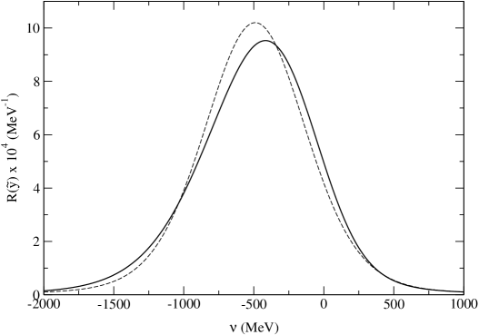
Figure 3: The exact response (solid curve) compared with the response obtained by folding the PWIA response with the approximate folding function $F_{A}$ of Eq.(29) for $\Gamma_{0}=100$ MeV.

In conclusion, we find that the effects of FSI, neglected in the PWIA, become independent of $|\mathbf{q}|$ at large $|\mathbf{q}|$ for a particle confined in a linear potential. They increase the width of the response, and must be removed before extracting momentum distributions or other target structure information from the observed response. In general one can always represent the FSI effects by a folding function; in this simple case a Gaussian folding function provides a reasonable approximation. Finally, the OSA predicts a response of the wrong shape but with correct values for the first three moments in the case of a linear potential.