A mixed-mode shell-model theory for nuclear structure studies

Abstract

We introduce a shell-model theory that combines traditional spherical states, which yield a diagonal representation of the usual single-particle interaction, with collective configurations that track deformations, and test the validity of this mixed-mode, oblique basis shell-model scheme on ²⁴Mg. The correct binding energy (within 2% of the full-space result) as well as low-energy configurations that have greater than 90% overlap with full-space results are obtained in a space that spans less than 10% of the full space. The results suggest that a mixed-mode shell-model theory may be useful in situations where competing degrees of freedom dominate the dynamics and full-space calculations are not feasible.

PACS numbers: 21.60.Cs, 21.60.Ev, 21.60.Fw, 27.30.+t

Keywords: mixed-mode, symmetry-mixing, degrees of freedom, non-perturbative,
non-orthogonal basis, generalized eigenvalue problem

Numerical methods: Cholesky, Lanczos

I Introduction

Every quantum mechanical problem involves the solution of an eigenvalue equation. In practice, there are only a few exactly solvable analytic models, and these are realized only rarely (if ever) in nature so one is often forced to consider numerical solutions. In addition, since in the latter case the dimensionality of a model space can be very large, especially when dealing with realistic systems such as nuclei where the number of particles is more than a few but less than what is needed to justify the use of statistical methods, it is frequently necessary to consider various approximations, including, especially, basis truncation.

The usual approach is to select a convenient orthonormal basis in which to carry out a calculation. The use of a non-orthogonal scheme, though in principle no more difficult than using an orthogonal one, is only justified if it is driven by physical considerations. For example, when a system supports competing modes and a ‘preferred’ basis can be associated with each, it makes sense to consider a non-orthogonal basis comprised of leading configurations of each of these modes. Finding a ‘good’ orthogonal basis, which is intimately related to a ‘good’ (but not exact) symmetries can be as difficult as solving the problem itself; nonetheless, this is usually key to understanding the dominant modes (underlying physics) of a system and outcomes of numerical calculations [1].

The mixed-mode system of interest to us seeks to accommodate the single-particle and collective-quadrupole degrees of freedom that dominate the low-energy structure of atomic nuclei [2]. Manifestations of important collective excitations can also be found in many other branches of physics [3]. The mixed-mode nature enters in nuclear physics because the single-particle and collective-quadrupole modes have similar excitation energies, both being small relative to intra-shell excitation energies [2, 4]. Both vibration and rotation are manifestations of the collective motion [5], vibrations being close to spherical shape oscillations and rotations being the periodic motion of a well-deformed intrinsic configuration about some axis [6]. While in principle these modes are reachable through multiple single-particle excitations, a full many-body theory is required to offer a proper interpretation of this collective motion [7, 8].

In this paper we explore the efficacy of a mixed-mode shell-model scheme by considering ²⁴Mg which is known to manifest strongly competing single-particle and collective degrees of freedom. In particular, we examine convergence of results towards those of full-space $0\hbar\omega$ $sd$-shell calculations as a function of the number of particles in excited single-particle levels and the number of irreducible representations (irreps) of SU(3). The results show that a relatively small oblique space gives the right relative energy for the K=2 band which leads to the correct order for all the low-energy levels. The structure of the states is further tested against the exact full-space results by examining the overlap of calculated eigenstates. We begin by reviewing the mathematical underpinning of the theory in the second section. Results are presented in the third section with conclusions and a discussion on applicability of the approach given in the fourth section.

II Mathematical background

The success of the current approach, which will be demonstrated in detail in the next section, can be traced to the fact that the spherical shell-model states are eigenstates of the one-body Hamiltonian ($\sum\varepsilon_{i}a_{i}^{+}a_{i}$) while the two-body part of the Hamiltonian ($\sum_{i,j}V_{kl,ij}a_{i}^{+}a_{j}^{+}a_{k}a_{l}$) is strongly correlated with $Q\cdot Q$ which is diagonal in the SU(3) basis [9]. By combining spherical shell-model states and SU(3) states one accommodates, from the onset, the dominant modes of the system.

The usual procedure for solving the eigenvalue problem $\hat{H}\vec{v}=\lambda\vec{v}$ is to cast it into the form of a matrix equation. In a non-orthogonal basis [10], this matrix form includes the overlap matrix, $\Theta_{ij}=\langle j|i\rangle$, and has the form $\sum_{j}[H_{ij}v_{j}-\lambda\Theta_{ij}v_{j}]=0$. For an orthonormal basis the overlap matrix becomes the identity matrix ($\Theta_{ij}\rightarrow\delta_{ij}$) and the matrix form of the eigenvalue problem is $\sum_{j}H_{ij}v_{j}=\lambda v_{i}$. When the overlap matrix $\Theta$ is positive-definite the Cholesky algorithm can be used to solve the generalized eigenvalue problem [11]. For large spaces this eigenvalue problem can be solved efficiently by using the Lanczos algorithm [12].

For the calculations reported here we use a double mixed-mode basis. The first set consists of spherical shell-model states (ssm – states) expressed in terms of spherical single-particle coordinates ($nlj$). The second set has a good SU(3) structure (su3 – states) which track nuclear deformation [13]; this basis set is given in terms of cylindrical single-particle coordinates. By construction both sets have the third projection $M_{J}$ of the system’s total angular momentum J as a good quantum number [14, 15]. Schematically, these basis vectors and their overlap matrix can be represented in the following way:

$${\rm basis\quad vectors} : {\rm\quad}\left(\begin{array}[]{l}e_{\alpha}:{\rm ssm\ -\ basis}\\ E_{i}:{\rm su3\ -\ basis}\end{array}\right),$$ (3)

$${\rm overlap\quad matrix} : {\rm\quad}\Theta=\left(\begin{array}[]{ll}{\bf 1}&\Omega\\ \Omega^{+}&{\bf 1}\end{array}\right),\qquad\Omega_{\alpha i}=e_{\alpha}\cdot E_{i},$$ (6)

$${\rm Hamiltonian\quad matrix} : {\rm\quad}H=\left(\begin{array}[]{ll}H_{ssm\times ssm}&H_{ssm\times su3}\\ H_{su3\times ssm}&H_{su3\times su3}\end{array}\right)=\left(\begin{array}[]{ll}H_{\alpha\beta}&H_{\alpha j}\\ H_{i\beta}&H_{ij}\end{array}\right).$$ (11)

In the above, $\alpha$ and $i$ span the following ranges: $\alpha=1$, …, dim(ssm – basis) and $i=1$, …, dim(su3 – basis).

Calculations in a nonorthogonal oblique-basis require an evaluation of the matrix elements of physical operators plus a knowledge of the scalar product ($e_{\alpha}\cdot E_{i}$). While it may be desirable to have an analytical expression for the overlap matrix, as we have for the single-particle overlap matrix [16], for practical purposes it suffices either to know the representation of each basis state in a common set that spans the full space, which is counter to the overall objective of reducing the number of basis states to a manageable subset, or to expand one set in terms of the other. For the present work, the $e_{\alpha}$, which can be represented by a single machine word in a spherical single-particle scheme, were expanded in a cylindrical basis, which is the representation for our collective SU(3) basis vectors. This transformation is handled by an efficient routine that exploits two computational aids: bit manipulation via logical operations and a weighted search tree for fast data storage and retrieval [17]. In the best case scenario a transformation of this type has to be done at least once per ssm basis state $e_{\alpha}$. We transform the ssm basis states since the result is usually a vector with fewer components than a typical SU(3) basis state. There is a simple way to calculate the overlap between states [18], however for the calculation of matrix elements it is better to transform each $e_{\alpha}$ vector in the basis used by the SU(3) states.

Matrix elements of the one-body and two-body Hamiltonian

$$H=\sum_{i}\varepsilon_{i}a_{i}^{+}a_{i}+\frac{1}{4}\sum_{i,j}V_{kl,ij}a_{i}^{+}a_{j}^{+}a_{k}a_{l}$$ (12)

have to be evaluated in each subspace ($H_{\alpha\beta}$ and $H_{ji}$) as well as between the spaces ($H_{\alpha i}$ and $H_{j\beta}$), see (11). The $H_{\alpha\beta}$ part is normally given and evaluated in a spherical single-particle basis. By transforming the Hamiltonian to a cylindrical single-particle basis one can obtain the $H_{ji}$ part of $H$. In order to compute the off-diagonal blocks $H_{\alpha i}$ and $H_{j\beta}$ and overlap matrix elements between SU(3) and ssm basis states, both basis sets are expanded in a basis of Slater determinants using cylindrical single-particle states. For the (8,4) and (9,2) irreps this is an expansion into 2120 Slater determinants at most; each ssm state, which itself is a single Slater determinant in a spherical single-particle basis, typically expands into a smaller number of cylindrical-basis Slater determinants which is less than 1296. We do not expand the SU(3) states into spherical-basis Slater determinants because that would require significant fraction of the entire spherical shell model space, defeating the rationale of our approach. Taking into account the significant number of Hamiltonian matrix elements ($H_{ij}$ and $H_{i\beta}$) between multi-component states, it should be clear that this is the most time consuming part of the calculation. The extra labels associated with the intrinsic quadrupole moment $\varepsilon$ of each basis state is used to produce well-structured band-like matrices and to speed up the calculation. Specifically, basis states are pre-ordered according to their deformation as reflected by $\varepsilon$ and during the evaluation of $H$ a $\Delta\varepsilon$ selection rule is applied.

It is important to point out that knowledge of the overlap matrix $\Theta$ and the matrix elements of $H$ in the two spaces ($H_{\alpha\beta}$, $H_{ij}$) is not enough to obtain the correct off-diagonal block $H_{\alpha i}.$ This is clear from the following explicit expression for $H_{\alpha i}$ which contains a summation along ($\bar{\beta}$) that lies outside of the ($\beta,i$) model spaces:

$$H_{\alpha i}=\sum_{\beta}H_{\alpha\beta}\Theta_{\beta i}+\sum_{\bar{\beta}}H_{\alpha\bar{\beta}}\Theta_{\bar{\beta}i}.$$ (13)

Thus a direct evaluation of $H_{\alpha i}$ is required.

It is instructive to consider a geometrical visualization of the oblique basis-state concept. Since a set of vectors defines a hyper-plane, it is natural to ask the question: “What is the angle between hyperplanes defined by the bases under consideration?” To answer this question, first consider the angle $\theta$ between a normalized SU(3) basis vector $\vec{v}$ and the subspace $V$ spanned by the spherical shell-model basis vectors. The length of the projected vector $\vec{v}_{V}\in V$ is given by $\cos(\vec{v},V)=\cos\theta=\left|\vec{v}_{V}\right|$. The space $V$ of the spherical shell-model basis vectors induces a natural basis $\vec{n}_{\varepsilon}$ in the SU(3) space ($\vec{n}_{\varepsilon}=n_{\varepsilon}^{i}\vec{E}_{i}$). The angle between each new basis vector $\vec{n}_{\varepsilon}$ and the space $V$ will again be the length of its projection into the space $V,$ but it has the nice property that this set of orthogonal basis vectors stays orthogonal after the projection into the space $V$:

$$\cos\theta_{\varepsilon} = \cos(\vec{n}_{\varepsilon},V)=\left|\vec{n}_{\varepsilon V}\right|,$$

$$\vec{n}_{\varepsilon V} = \sum_{i,\alpha}n_{\varepsilon}^{i}(\vec{E}_{i}\cdot\vec{e}_{\alpha})\vec{e}_{\alpha}=\sum_{i,\alpha}n_{\varepsilon}^{i}\Theta_{i\alpha}\vec{e}_{\alpha},$$

$$\left|\vec{n}_{\varepsilon V}\right|^{2} = \sum_{\alpha}(\sum_{i}n_{\varepsilon}^{i}\Theta_{i\alpha})^{2}=\sum_{\alpha,i,j}n_{\varepsilon}^{i}\Theta_{i\alpha}n_{\varepsilon}^{j}\Theta_{j\alpha}.$$

In matrix notation this reads

$\displaystyle\left|\vec{n}_{\varepsilon V}\right|^{2}=\vec{n}_{\varepsilon}\cdot\hat{\Theta}\cdot\hat{\Theta}^{T}\cdot\vec{n}_{\varepsilon},$

where the natural basis vectors $\vec{n}_{\varepsilon}$ are eigenvectors of the symmetric matrix $\hat{\Theta}\cdot\hat{\Theta}^{T}$

$$\hat{\Theta}\cdot\hat{\Theta}^{T}\cdot\vec{n}_{\varepsilon}=\varepsilon^{2}\vec{n}_{\varepsilon}.$$ (14)

It follows that $\left|\vec{n}_{\varepsilon V}\right|^{2}=\vec{n}_{\varepsilon}\cdot\hat{\Theta}\cdot\hat{\Theta}^{T}\cdot\vec{n}_{\varepsilon}=\varepsilon^{2}\vec{n}_{\varepsilon}\cdot\vec{n}_{\varepsilon}=\varepsilon^{2}$ and thus the matrix $\hat{\Theta}\cdot\hat{\Theta}^{T}$ is positive definite ($\left|\vec{n}_{\varepsilon V}\right|^{2}=\varepsilon^{2}\geq 0$ ) with eigenvalues determined by the $\cos\theta.$ This construction allows for a simple visualization of the oblique basis space: Choose the $x-$axis to correspond to the space $V$ of all the spherical shell-model basis vectors and represent the SU(3) space as a collection of unit vectors each at an angle $\cos\theta=\varepsilon$ with respect to the $x-$axis. In the next section this construction will be applied to the geometry of oblique basis space calculations to demonstrate the relative orthogonality of the two vector sets, $e_{\alpha}$ and $E_{i}$.

III An illustrative example

In this section the oblique-basis technique is tested for ²⁴Mg, which is a strongly deformed nucleus with well-known collective properties and one of the best manifestations of the Elliott’s SU(3) symmetry [8]. In terms of dimensionality of the model space, adding a few leading SU(3) irreps to a highly truncated spherical shell-model basis results in significant gains in the convergence of the low-energy spectra towards the full space result. In particular, the addition of leading SU(3) irreps yields the right placement of the K=2 band and the correct order for most of the low-lying levels. Indeed, an even more detailed analysis shows that the structure of the low-lying states is significantly improved through the addition of a few SU(3) irreps. The Hamiltonian used in our analysis is the Wildenthal interaction [19].

Our model space for ²⁴Mg consists of 4 valence protons and 4 valence neutrons in the $0\hbar\omega$ $sd$-shell. The $m$-scheme dimensionality ($M_{J}=0$) of this space is 28503 which in the figures that follow is denoted FULL. To test the effects of truncations, calculations were also carried out on permitting $n$ particles to be excited out of the lowest $d_{5/2}$ orbit, i.e. $d_{5/2}^{8-n}(d_{3/2}s_{1/2})^{n}$, and are denoted as SM(n). The SM(2) approximation is of particular interest since it allows one to take into account the effect of pairing correlations (one pair max) in the ‘secondary levels’ ($s_{1/2}$ and $d_{3/2}$ for the ds shell) with a minimum expansion of the model space. The SU(3) part of the basis includes two scenarios: one with only the leading representation of SU(3) included, which for ²⁴Mg is the (8,4) irrep with dimensionality 23 for the $M_{J}=0$ space and denoted in what follows by appending (8,4) to the corresponding SM(n) notation; and another with the (8,4) irrep plus the next most important representation of SU(3), namely the (9,2). The (9,2) irrep occurs three times, once with S=0 ($M_{J}=0$ dimensionality 15) and twice with S=1 ( $M_{J}=0$ dimensionality $2\times 45=90$). All three (9,2) irreps have total $M_{J}=0$ dimensionality of 15+90=105. The (8,4)&(9,2) case has total $M_{J}=0$ dimensionality of 23+105=128 and is denoted by appending (8,4)&(9,2) to the corresponding SM(n) notation. In Table I we summarize the dimensionalities involved.

TABLE I.: Labels used to distinguish various calculations and the corresponding $M_{J}=0$ dimensionalities. The leading SU(3) irrep is denoted by (8,4) while (8,4)&(9,2) implies that (9,2) irreps have also been included. The SM(n) spaces correspond to spherical shell-model partitions with $n$ valence particles excited out of the $d_{5/2}$ shell into the $s_{1/2}$ and $d_{3/2}$ levels.

Model space		$(8,4)$		$(8,4)\&(9,2)$		$SM(0)$		$SM(1)$		$SM(2)$		$SM(4)$		$FULL$
space dimension		$23$		$128$		$29$		$449$		$2829$		$18290$		$28503$
% of the full space		$0.08$		$0.45$		$0.10$		$1.57$		$9.92$		$64.17$		$100$

Now, the method described at the end of the previous section is used to visualize the structure of the oblique basis space. First consider the SM(2) space enhanced by the SU(3) irreps (8,4)&(9,2). Since the SM(2) and (8,4)&(9,2) spaces are both relatively small (see Table I) we expect the basis vectors in these spaces to be nearly orthogonal. This orthogonality is clearly seen from inset (a) in Fig.1. Inset (b) in Fig.1 shows a loss of orthogonality between the SM(4) and the (8,4)&(9,2) basis vectors. This is due to the fact that SM(4) space is about 64% of the full $sd$-space and therefore there is a relatively high probability that some linear combinations of the SU(3) basis vectors lie in the SM(4) space. Indeed, it can be shown that there are five vectors from (8,4)&(9,2) that lie within the SM(4) space. Such redundant vectors must, of course, be excluded from the calculation.

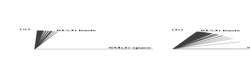
FIG. 1.: Orthogonality of the basis vectors in the oblique geometry. The SU(3) space consist of (8,4)&(9,2) basis vectors with the shell-model spaces (SM(n) with n=2 and 4) indicated by a horizontal line. (a) SM(2) and the natural SU(3) basis vectors and (b) SM(4) and the natural SU(3) basis vectors. In the latter case there are five SU(3) vectors that lie in the SM(4) space.

We now turn to a consideration of the main results of the oblique basis calculation, starting with ground-state convergence issues. The results shown in Fig.2 illustrate that the oblique basis calculation gives good dimensional convergence in the sense that the calculated ground-state energy for the SM(2)+(8,4)&(9,2) calculation is 3.3 MeV below that calculated energy for the SM(2) space alone. Adding the SU(3) irreps only increases the size of the space from 9.9% to 10.4% of the full space. This 0.5% increase in the size of the space is to be compared with the huge (54%) increase in going from SM(2) to a SM(4) calculation. For the later the ground state energy is 4.2 MeV lower than SM(2) result, somewhat better than for the SM(2)+(8,4)&(9,2) calculation but in 64.2% rather than 10.4% of the full model space.

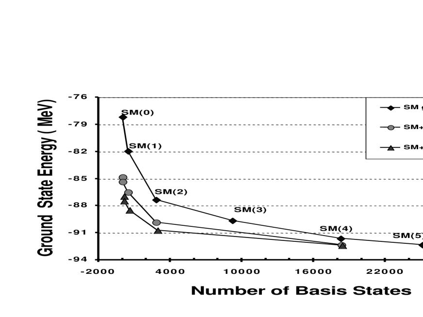
FIG. 2.: Calculated ground-state energy for ²⁴Mg as a function of the various model spaces. Note the dramatic increase in binding (3.3 MeV) in going from SM(2) to SM(2)+(8,4)&(9,2) (a 0.5% increase in the dimensionality of the model space). Enlarging the space from SM(2) to SM(4) (a 54% increase in the dimensionality of the model space) adds 4.2 MeV in binding energy.

Figs. 3 and 4 show that the oblique basis calculation positions the K=2 band head correctly. Furthermore, most of the other low-energy levels are also positioned correctly. The results for pure spherical and pure SU(3) calculations are shown in Fig.3. As can be see from the Fig.3 results, an SM(4) calculation (64% of the full model space) is needed to get the ordering of the lowest angular momentum states correct. Also notice that in this case the 3th and 4th energy levels are practically degenerate. On other hand, it only takes 0.5% of the full space to achieve comparable success with SU(3). In particular, Fig.3 shows that an SU(3) calculation using only the (8,4) and (9,2) irreps gives the right ordering of the lowest levels. Note that the first few low-energy levels for SM(2) are close in energy to the corresponding low-energy levels for the (8,4)&(9,2) result. Since these two spaces are nearly orthogonal (see Fig.1), these two sets of levels mix strongly in an oblique calculation and yield excellent results. The comparable ground-state energies of the SM(2) and (8,4)&(9,2) configurations can also be seen from Fig.2.

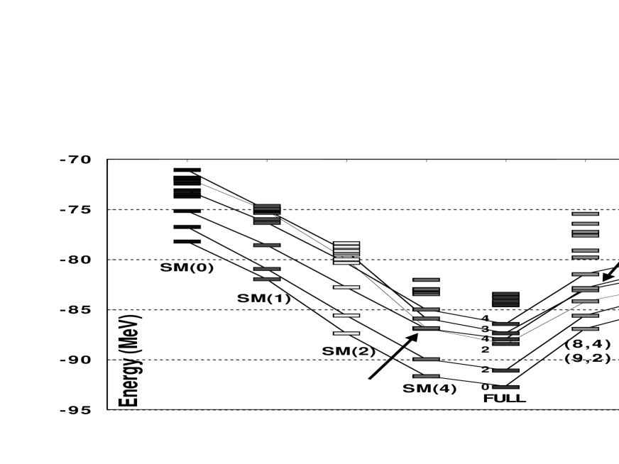
FIG. 3.: Structure of the energy levels for ²⁴Mg: pure $m$-scheme spherical basis space calculations are on the left-hand side of the graph; pure SU(3) basis space calculations are on the right-hand side; the spectrum from the FULL space calculation is in the center.

The spectra shown in Fig.3 are to be compared with the results from the oblique basis calculations shown in Fig.4. From this comparison one can see that the correct level structure can be achieved by using 1.6% (SM(1)+(8,4)) of the full $sd$-space. However, one should also notice that for the SM(0)+(8,2) space, which is only 0.2% of the full space and the minimum oblique basis calculation, the results are quite close to the correct level structure. Despite the fact that the ground state energy of the oblique basis calculations is higher than the ground state energy for the SM(4) type calculation, the oblique calculations are favorable in terms of dimensionality considerations and correctness of the level structure.

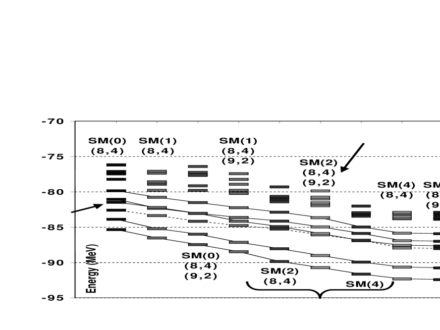
FIG. 4.: Energy levels for ²⁴Mg as calculated for different oblique bases. The SM(4) basis calculation is included for comparison.

Figs. 5–8 focus on the actual structure of the states by showing overlaps of eigenstates calculated in the SM(n), SU(3), and oblique bases with the corresponding states of the full space calculation. Specifically, in Fig.5 overlaps of states for pure SM(n) and pure SU(3) type calculations are given. Note that the SM(4) states have big overlap (90%) for the first few eigenstates. This should not be too surprising since SM(4) covers 64% of the full space.

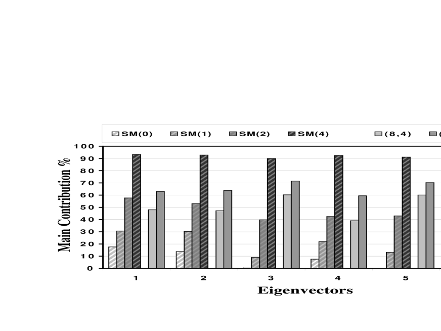
FIG. 5.: Overlaps of the pure spherical shell-model and pure SU(3) eigenstates with the corresponding FULL space results for ²⁴Mg. The first four bars represent the SM(0), SM(1), SM(2), and SM(4) calculations, the next three bars represent SU(3) calculations, etc.

The results of Fig.5 show that in general SU(3) based calculations give much better results then low-dimensional SM(n)-type calculations. The SM(n) based calculations have irregular overlaps along the low-lying states and require SM(4), which is 64% of the full space, to get relatively well behaved overlaps. This can be seen most clearly from the inset labeled SM in Fig.6. Note that the SM(0) contributions to the third, fifth and sixth states are very low, while SM(1) and SM(2) have varying contributions. The structure of states obtained in any SU(3)–type calculation leads to a stable picture for the oblique calculations as shown in the inset SM(n)+(8,4) and SM(n)+(8,4)&(9,2) in Fig.6.

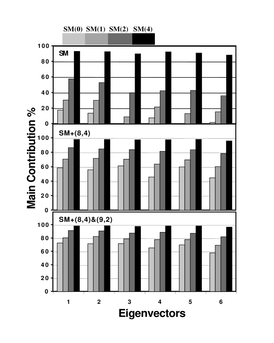
FIG. 6.: Overlaps of calculated eigenstates for oblique basis calculations with the exact results from FULL $sd$-shell calculations. Inset SM contains the overlaps for the pure spherical shell-model basis states only. Inset SM+(8,4) contains the overlaps of the SM basis enhanced by the leading SU(3) irrep (8,4). Inset SM+(8,4)&(9,2) has the (9,2) irreps included as well.

In Fig.7 the improvement in the structure of the calculated states is followed as the SU(3) states are added to the SM(n) basis. From this graph one can see that the improvement to the SM(0)– and SM(1)-type calculation is due mainly to the goodness of SU(3) itself. The improvement obtained in the oblique calculation is due to the SU(3) enhancement of the SM(2) space. From this graph one can also conclude that there is only a small gain in going to the SM(4) based oblique calculation. However, this improvement can not be achieved by any other means with such a small increase in the model space. This is clear from a careful examination of Fig.2 where one can see that the SM(5) result, which has 25142 basis vectors (88% of the full $sd$-space), gives the same ground-state energy as the SM(4)+(8,4)&(9,2) result (64.6% of the full $sd$-space).

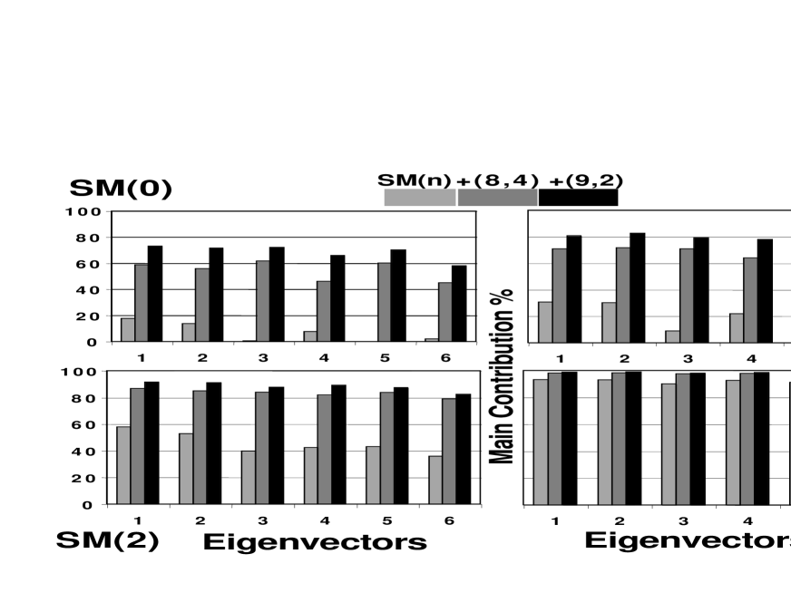
FIG. 7.: Overlaps of oblique basis states with the exact eigenstates from the FULL $sd$-shell calculation. Each inset represents a particular SM(n)–type calculation, showing how the overlaps change along the corresponding oblique basis calculation.

Finally, to compare the three schemes – SU(3), SM(n) and the various oblique basis combinations – representative overlaps are shown in Fig.8. From these results it is very clear that SU(3)-type basis states yield the right structure in very low order. In particular, in Fig.8 it can be seen that a 90% overlap with the exact eigenvectors can be achieved by using only 10% of the total space, SM(2)+(8,4)&(9,2). Furthermore, Fig.8 also shows that SU(3) enhances the SM(4) results yielding eigenstates with overlaps that are very close ( $\approx$ 98%) to the exact results.

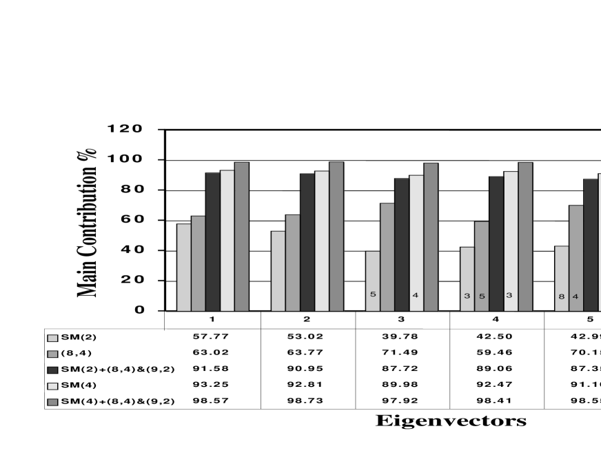
FIG. 8.: Representative overlaps of pure SM(n), pure SU(3), and oblique basis results with the exact full $sd$-shell eigenstates. Numbers within some of the bars reflect the miss-ordering of the corresponding spectrum with respect to the exact result. The number points to the actual state that has the overlap shown by the bar, this is the maximal overlap observed.

IV Conclusion and Discussions

In this paper we have shown that knowledge about the important modes of a physical system can be used to obtain good eigenstates in relatively small model spaces. In particular, for the ²⁴Mg example with typical one-body and two-body interactions, the proposed oblique scheme gives good dimensional convergence for the ground state energy, good spectral structure for all the low-energy states, and good overlaps of these states with full $sd$-shell calculations.

There are some natural choices for further development of the theory and its application. The most straightforward is a study of other $sd$-shell nuclei as well as $pf$-shell nuclei. Such studies will further test the theory and the codes that have been develop. These are currently underway. Another possibility is to integrate the oblique basis concept into no-core calculations of the type developed by [20]. Such an extension would involve the symplectic group for multi-shell correlations rather than just SU(3) [21]. A third even broader extension of the theory would involve a general procedure for the identification of dominant modes from any one- and two-body Hamiltonian along with a complementary partitioning of the model space into physically relevant subspaces with small overlaps. One can then start with eigenstates for an arbitrary subspace and constructively improve the results by including corrections from the remaining subspaces. It should be possible to do this by keeping only a small set of the calculated lowest energy states at each iteration.

The results presented here show very clearly that when important modes can be isolated one can build an oblique theory that incorporates leading configurations of each mode and get good convergence in a limited model space.

Support provided by the Department of Energy under Grant No. DE-FG02-96ER40985, and the National Science Foundation under Grant No. PHY-9970769, and by Cooperative Agreement EPS-9720652 that includes matching from the Louisiana Board of Regents Support Fund.

REFERENCES

- [1] J. P. Elliott, Symmetry in physics, (New York, Oxford University Press, 1979); G. K. Georges, W. Krauth and M. Rozenberg, Rev. Mod. Phys. 68, 13 (1996); D. J. Rowe, Rep. Prog. Phys. 48, 1419 (1985); J. P. Draayer, K. J. Weeks and G. Rosensteel, Nucl. Phys. A413, 215 (1984); S. Goshen and H. J. Lipkin, Ann. Phys. 6, 301 (1959); P. Van Isacker, Rep. Prog. Phys. 62, 1661 (1999).
- [2] A. Bohr and B. R. Mottelson, Nuclear structure (New York, W. A. Benjamin, 1969); A. M. Lane, Nuclear theory; pairing force correlations and collective motion (New York, W. A. Benjamin, 1964).
- [3] D. F. Phillips, A. Fleischhauer, A. Mair, R. L. Walsworth, and M. D. Lukin, Phys. Rev. Lett. 86, 783 (2001); M. Tinkham, Introduction to superconductivity (New York, McGraw Hill, 1996); A. S. Alexandrov, High temperature superconductors and other superfluids (London, Taylor & Francis, 1994); I. M. Khalatnikov, An introduction to the theory of superfluidity (New York, W. A. Benjamin, 1965); A. Griffin, Excitations in a Bose-condensed liquid (New York, Cambridgeshire University Press, 1993); NATO Advanced Study Institute, Collective excitations in solids (New York, Plenum Press, 1982); S. Lundqvist, Collective phenomena in non-uniform systems in Electron correlations in solids, molecules, and atoms Proceedings of a NATO Advanced Study Institute on Electron Correlations in Solids, Molecules, and Atoms, held at Corsendonk Conference Center, between July 20-31, 1981, in Turnhout, Belgium. (New York, Plenum Press, 1983); G. P. Harnwell, Atomic physics; an atomic description of physical phenomena (New York, McGraw-Hill, 1955); B. R. Judd, Topics in atomic & nuclear theory (Canterbury, N. Z. , University of Canterbury, 1970)
- [4] S. T. Beliaev, Collective excitations in nuclei (New York, Gordon and Breach, 1968); P. Ring and P. Shuck, The nuclear many-body problem (New York, Springer-Verlag, 1980); F. Iachello, The interacting boson model (New York, Cambridgeshire University Press, 1987); D. Bonatsos, Interacting boson models of nuclear structure (New York, Oxford University Press, 1988); A. Frank, Algebraic methods in molecular and nuclear structure physics (New York, Wiley, 1994); R. Casten, Nuclear structure from a simple perspective (New York, Oxford University Press, 1990).
- [5] Enrico Fermi International School of Physics, Elementary modes of excitation in nuclei (Amsterdam, North-Holland Pub. Co. , 1977).
- [6] J. P. Davidson, Collective models of the nucleus (New York, Academic Press, 1968); F. Iachello, The interacting Boson-Fermion model (New York, Cambridge University Press, 1991).
- [7] R. Leblanc, J. Carvalho, M. Vassanji, D. J. Rowe, Nucl. Phys. A 452 263 (1986); P. Park, J. Carvalho, M. Vassanji, D. J. Rowe, G. Rosensteel, Nucl. Phys. A 414, 93 (1984).
- [8] J. P. Elliott, Proc. Roy. Soc. London Ser. A 245, 128 (1958); 245, 562 (1958); J. P. Elliott and H. Harvey, ibid 272, 557 (1963); J. P. Elliott and C. E. Wilsdon, ibid 302, 509 (1968).
- [9] A. Cortes, R. U. Haq, and A. P. Zuker, Phys. Lett. B 115, 1 (1982).
- [10] L. Fox, An introduction to numerical linear algebra (Oxford, Clarendon Press, 1964); L. Fox and D. F. Mayers, Computing methods for scientists and engineers (Oxford, Clarendon Press, 1968).
- [11] W. H. Press, S. A. Teukolsky, W. T. Vetterling and B. P. Flannery, Numerical Recipes in Fortran 77: The Art of Scientific Computing , Volum 1 (Cambridge University Press 1992); http://www. nr. com
- [12] R. R. Whitehead et al. , Adv. Nucl. Phys. 9, 123 (1977); G. H. Golub, and C. F. Van Loan, Matrix Computations (Baltimor and London, The Johns Hopkins University Press, 1989); Jane K. Cullum, Lanczos algorithms for large symmetric eigenvalue computations (Boston, Birkhäuser, 1985).
- [13] J. P. Draayer, S. C. Park, and O. Castanos, Phys. Rev. Lett. 62, 20 (1989).
- [14] B. A. Brown and B. H. Wildenthal, Ann. Rev. Nucl. Part. Sci. 38, 29 (1988).
- [15] V. G. Gueorguiev and J. P. Draayer, Rev. Mex. Fis. (Suppl. 2) 44, 43 (1998).
- [16] E. Chacon, Rev. Mex. Fis. 12, 57 (1963).
- [17] S. C. Park, J. P. Draayer, S.-Q. Zheng, C. Bahri, Comput. Phys. Commun. 82, 247 (1994)
- [18] G. H. Lang, C. W. Johnson, S. E. Koonin, and W. E. Ormand, Phys. Rev.C 48, 1518 (1993); E. Y. Loh, Jr. and J. E. Gubernatis, in Electronic Phase Transitions, edited by W. Hanke and Yu. V. Kopaev (Elsevier Science Publishers, New York, 1992).
- [19] B. H. Wildenthal, Prog. Part. Nucl. Phys. 11, 5 (1984); wpn interaction file from B. A. Brown via http://www. nscl. msu. edu/~brown/database.htm.
- [20] P. Navratil, J. P. Vary, B. R. Barrett, Phys. Rev. Lett. 84, 5728 (2000); P. Navratil, J. P. Vary, B. R. Barrett, Phys. Rev. C 62, 4311 (2000).
- [21] J. Escher and J. P. Draayer, J. Math. Phys. 39, 5123 (1998); G. Rosensteel and D. J. Rowe, On the algebraic formulation of collective models. III. The symplectic shell model of collective motion, Ann. Phys. 126, 343 (1980).