A Hydrodynamic Description of Heavy Ion Collisions at the SPS and RHIC

Abstract

A hydrodynamic + cascade model of relativistic heavy ion collisions is presented and compared to available hadronic data from the SPS to RHIC. The model consistently reproduces the radial and elliptic flow data for different particles, collision energies, and impact parameters. Three ingredients are essential to the success: (a) a reasonable EOS exhibiting the hard and soft features of the QCD phase transition, (b) thermal hadronization at the phase boundary, and (c) subsequent hadronic rescattering. Some features of the RHIC data are readily explained: (i) the observed elliptic flow and its dependence on $p_{T}$ and mass, (ii) the anomalous $\bar{p}/\pi^{-}$ ratio for $p_{T}\approx 2.0\,\mbox{GeV}$, (iii) the difference in the slope parameters measured by the STAR and PHENIX collaborations, and (iv) the respectively strong and weak impact parameter dependence of the $\bar{p}$ and $\phi$ slope parameters. For an EOS without the hard and soft features of the QCD phase transition, the broad consistency with the data is lost.

I Introduction

I.1 Reaching the Macroscopic Limit

Excited nuclear matter has been created by colliding Pb and Au ions at the SPS ($\sqrt{s}=17\,\mbox{GeV per nucleon}$) and RHIC ($\sqrt{s}=130\,\mbox{GeV per nucleon}$) accelerators QM97 ; QuarkMatter99 ; QM2001 . For infinitely large nuclei, the excited matter can be characterized by macroscopic quantities – pressure, temperature, viscosity, etc. Lattice QCD simulations indicate that for temperatures larger than $T_{c}\approx 160~{}\mbox{MeV}$, confined nuclear matter morphs into a phase of deconfined quarks and gluons – the Quark Gluon Plasma (QGP) ShuryakQGP ; Lattice-Eos . The possibility of observing the QGP in real nuclei has motivated the heavy ion experimental program.

If the system is macroscopic then thermodynamics describes the static properties of the matter and hydrodynamics describes the dynamic properties of the matter. In fact, the observed particle ratios are remarkably close to the particle ratios in an ideal gas of hadrons at a temperature, $T\approx 165\,\mbox{MeV}$ Stachel-Thermal ; Becattini-Thermal ; Sollfrank-Thermal ; Redlich-Thermal . This suggests that the system evolved from a state close to thermal equilibrium at the phase transition boundary. However, the same thermal description reproduces the hadron ratios in proton-proton and $e^{+}e^{-}$ collisions, where the system size is small and equilibration seems impossible. The success of thermodynamics seems to reflect phase space rather than the equilibration of macroscopic system.

Therefore, a thermodynamic (static) description, divorced from a hydrodynamic (dynamic) description, can not unambiguously signal a macroscopic state. It is important that elementary proton-proton and $e^{+}e^{-}$ collisions do not exhibit hydrodynamic behavior. An analysis of hadronic spectra SZ-FlowProfile shows little sign of the transverse expansion predicted by hydrodynamics. Thus, the excited systems produced in these elementary collisions are $not$ macroscopic.

In contrast, experiments with heavy ions do show evidence for a hydrodynamic expansion. Momentum correlations, colloquially known as $flow$, are observed at the SPS and RHIC. In PbPb collisions, the particles emerge from the collision with a collective transverse velocity of approximately $1/2\,c$ RadialFlow-Review . This radial flow is firmly established from a combined analysis of particle spectra, HBT correlations, and deuteron coalescence Uli-Expand . In non-central collisions, the particles emerge with an elliptic flow (see for exampleQuarkMatter99 ; QM2001 ). Elliptic flow is quantified by $v_{2}$, the asymmetry of the angular distribution

$$v_{2} = \left\langle\cos(2\,\phi)\right\rangle$$ (1)

where $\phi$ is measured around the beam axis with respect to the impact parameter. Radial and elliptic flow data are measured as a function of transverse momenta, particle type, impact parameter, and collision energy. This wealth of momentum correlations severely constrains viable models of the heavy ion collision.

Several microscopic models have been used to explain the available heavy-ion data. The first is a dilute parton model, which is quantified with the HIJING event generator HIJING . Dilute parton models are based upon the extrapolation of perturbative QCD from high $p_{T}$ down to a scale of $\sim 1\,\mbox{GeV}$. For central AuAu collisions at RHIC, HIJING predicted a mini-jet multiplicity of $\frac{dN^{g}}{dy}\sim 200$, which is insufficient to generate the strong hydrodynamic response observed at RHIC Molnar-Elliptic . The second is a string model, which is quantified with the UrQMD event generator. In string-models non-interacting strings decay into hadrons which subsequently interact. Due to the small transverse pressure at early times, UrQMD predicted a decrease in elliptic flow from the SPS to RHIC UrQMD-Elliptic . A $\approx 50\%$ increase was observed. In contrast to these microscopic models, hydrodynamic calculations at the SPS and RHIC, give a good description of the observed radial and elliptic flows Sollfrank-BigHydro ; Schlei-BigHydro ; Kolb-UU ; Kolb-LowDensity ; Kolb-Radial ; Htoh , but offer no insight into the microscopic mechanism of equilibration.

Accepting the macroscopic approach and its limitations, the phase transition to the QGP influences both the radial and elliptic flows. Lattice simulations indicate Lattice-Eos that over a wide range of energy densities $e=0.5-1.3\,\mbox{GeV/fm}^{3}$, the temperature and pressure are nearly constant and the speed of sound is approximately zero, $\frac{dp}{de}\approx 0$. Because the speed of sound is small in this range, the pressure can not effectively accelerate the matter HS-soft ; Rischke-Log . However, when the initial energy density is well above the transition region, the matter enters the hard QGP phase. The speed of sound approaches $\sqrt{1/3}$ and the pressure drives collective motion. At a time of $\sim 1~{}\mbox{fm/c}$, the energy density at the SPS and RHIC are very approximately $4$ and $8~{}\mbox{GeV/fm}^{3}$ NA49-EnergyDensity ; Phobos-Multiplicity . Based on these experimental estimates, the hard QGP phase is expected to live significantly longer at RHIC than at the SPS. The final radial and elliptic flows of the produced particles should reflect this difference VanHove-T ; Ollitrault-MixedPhase ; Kataja-MixedPhase ; Ollitrault-Elliptic ; Kolb-UU ; Rischke-Px .

Certainly, hydrodynamics is not applicable when the particles decouple from the collision and this “freezeout” must be modeled in order to compare the observed hadron spectra to hydrodynamic calculations. Usually, a naive freezeout prescription is taken: A “freezeout Temperature” $T_{f}$, is specified; thermal and chemical equilibrium are assumed for $T<T_{f}$; the spectrum of particles passing through the $T_{f}$ isotherm is calculated; $T_{f}$ is finally adjusted to match the single particle spectrum of pions and nucleons. Of course, this prescription is unrealistic and takes away from the predictive power of hydrodynamics. Nevertheless, the approach successfully describes many radial and elliptic observables from the SPS to RHIC Sollfrank-BigHydro ; Schlei-BigHydro ; Kolb-LowDensity ; Kolb-Radial .

However, the naive freezeout prescription fails in a number of respects. First, on the time scale of the collision $\sim 10~{}\mbox{fm/c}$, hadronic reactions do not alter the hadron composition and chemical equilibrium is not maintained (see for example Uli-Chemical ; HydroUrqmd ; UrQMD-Hagedorn ). Therefore in the late hadronic stages, chemical freezeout must be modeled in order to describe the resonance contribution and the particle ratios. Second, different particle types freezeout at different times and with different transverse velocities. With a universal freezeout temperature, the transverse flow of the strange particles $\Lambda,\,\Xi,\,\Omega$, is never reproduced Sorge-Strange . Third, at the SPS and RHIC, integrated elliptic flow is a strong function of the freezeout temperature. When the universal freezeout temperature is adjusted to match the nucleon spectrum, the integrated pion elliptic flow is too large Kolb-Flow . In reality, pions and nucleons freezeout at different times and temperatures.

To model freezeout, Bass and Dumitru HydroUrqmd replaced the hadronic phase of the hydrodynamics with a hadronic transport model, UrQMD. In this approach, the switch from hydro to cascade is made at a switching temperature, $T_{switch}\approx T_{c}$. The spectrum of particles leaving the surface is taken as the input to the cascade and the attendant theoretical problems are ignored. The approach worked. Chemical freezeout was incorporated into a comprehensive dynamical picture. The flow of the multi-strange baryons was reproduced. When a similar hydro+cascade model Htoh was applied to non-central collisions, elliptic flow was also reproduced at the 20% level. Furthermore, with the $T_{f}$ indeterminacy removed, these “simple” boost invariant hydro+cascade models were rather predictive – only $\frac{dN}{dy}$ and the $\bar{p}/p$ ratio have to be specified.

I.2 Brief Summary

In this work, we compare the hydro+cascade model of Htoh to the flow systematics at the SPS and RHIC. The model uses hydrodynamics to model the initial stage of the collision, and the hadronic cascade, Relativistic Quantum Molecular Dynamics (RQMD v2.4), to model the final stages of the collision Sorge-RQMD .

The Equation of State (EOS) is varied systematically and results are compared to the whole body of flow data from the SPS to RHIC. A family of EOS, labeled by the value of the Latent Heat (LH) is constructed; LH4, LH8, LH16$...$ denote increasingly soft EOS with latent heats $0.4,0.8,1.6...\,\mbox{GeV/fm}^{3}$ respectively. As a limiting case, the latent heat is made very large forming LH$\infty$. A Resonance Gas (RG) EOS is also studied. For an EOS with both the hard and soft features of the QCD phase transition, the model is broadly consistent with the body of available data. The best overall consistency with the data is found with LH8. For an EOS with only hard (e.g. RG) or only soft features (e.g. LH$\infty$), the broad consistency with the data is lost.

The model consists of three distinct components. The first component solves the equations of relativistic hydrodynamics in the transverse plane, assuming Bjorken scaling Bjorken-83 . The switching surface, or the isotherm where $T_{switch}=160\,\mbox{MeV}$, is found. The sensitivity of the model results to $T_{switch}$ will be discussed in a separate publication where chemical freezeout is also addressed Teaney-Chemical . The second component converts the macroscopic hydrodynamic variables on the switching surface into hadrons according to the Cooper-Frye prescription augmented with a theta function rejecting backward moving particles CooperFrye . Finally, the third component, the hadronic cascade RQMD sequentially rescatters the generated hadrons and models the hadronic freezeout stage of the collision. Throughout the analysis the role of hadronic rescattering is assessed. In all figures, the “Hydro+RQMD” curves incorporate hadronic rescattering and resonance decays while the “Hydro Only” curves only incorporate resonance decays.

As outlined in the abstract, several features of the first RHIC data are readily explained in the course of this analysis.

II Model Description and the EOS

II.1 Hydrodynamics

Relativistic hydrodynamics is a set of conservation laws for the stress tensor ($T^{\mu\nu}$) and for the conserved currents ($J_{i}^{\mu}$), $\partial_{\mu}T^{\mu\nu}=0$ and $\partial_{\mu}J_{i}^{\mu}=0$. In equilibrium, $T^{\mu\nu}$ and $J_{i}^{\mu}$ are related to the bulk properties of the fluid by the relations, $T^{\mu\nu}=(\epsilon+p)U^{\mu}U^{\nu}-pg^{\mu\nu}$ and $J_{i}^{\mu}=n_{i}U^{\mu}$ LL-Hydro . Here $\epsilon$ is the energy density, $p$ is the pressure, $n_{i}$ is the number density of the corresponding current, and $U^{\mu}=\gamma(1,\bf{v})$ is the proper velocity of the fluid. In strong interactions, the conserved currents are isospin ($J_{I}^{\mu}$), strangeness ($J_{S}^{\mu}$), and baryon number ($J_{B}^{\mu}$). For the hydrodynamic evolution, isospin symmetry is assumed and the net strangeness is set to zero; therefore only the baryon current $J_{B}$ is considered below.

The equations of motion may be expressed in terms of the variables $\tau=\sqrt{t^{2}-z^{2}}$ and $\eta=\frac{1}{2}\log(\frac{t+z}{t-z})$, which are respectively referred to as the Bjorken proper time and the spatial rapidity. Boost invariance assumes that the solution for any value of $\eta$ may be found by boosting the solution at $\eta=0$ to a frame moving with velocity $v=\tanh(\eta)$ in the negative z-direction. With this assumption, the equations of motion become two dimensional Bjorken-83 ; Ollitrault-Elliptic and are given at $\eta=0$ by

$$\partial_{\tau}(\tau T^{00})+\partial_{x}(\tau T^{0x})+\partial_{y}(\tau T^{0y}) = -p$$ (2)

$$\partial_{\tau}(\tau T^{0x})+\partial_{x}(\tau T^{xx})+\partial_{y}(\tau T^{xy}) = 0$$

$$\partial_{\tau}(\tau T^{0y})+\partial_{x}(\tau T^{xy})+\partial_{y}(\tau T^{yy}) = 0$$

$$\partial_{\tau}(\tau J_{B}^{0})+\partial_{x}(\tau J_{i}^{B})+\partial_{y}(\tau J_{B}^{y}) = 0\,.$$

Integrating over the transverse plane, one finds that net baryon number per unit spatial rapidity, $\int dxdy\,(\tau J_{B}^{0})$, and the transverse momentum per unit rapidity, $\int dxdy\,(\tau T^{0x})$ as well as $\int dxdy\,(\tau T^{0y})$, are conserved. The energy per unit rapidity, $\int dxdy\,(\tau T^{00})$, decreases due to the work done per unit time MG84-Work by the pressure in the longitudinal direction, $\int dxdy\,p$.

For an ideal fluid, entropy conservation can be derived LL-Hydro , $\partial_{\mu}(S^{\mu})=0$. The entropy current is defined as $S^{\mu}\equiv s\,U^{\mu}$, where $s$ is the entropy density and $U^{\mu}$ is the fluid 4-velocity. For a Bjorken expansion entropy conservation becomes

$$\partial_{\tau}(\tau S^{0})+\partial_{x}(\tau S^{x})+\partial_{y}(\tau S^{y}) = 0\,.$$ (3)

Integrating over the transverse plane, we find that

$$\int dx\,dy\,\tau\,s\gamma = \frac{dS_{tot}}{d\eta}$$ (4)

is a constant of the motion. This relation is monitored to test the accuracy of the solution.

These equations are solved numerically with a Gudunov method Hydro-Leveque . Using second order operator splitting Hydro-Leveque , a single time step separately updates the x-direction, the y-direction, and the loss terms on the r.h.s. of Eq. 2. Different splittings gave only negligibly different results. The simple RHLLE Riemann solver was used for the updates in the x and y directions Rischke-RHLLE ; Rischke-PlasmaTest . A second order (in $\tau$) Runge-Kutta stepper was used for the r.h.s. update.

II.2 Initial Conditions

To model the initial conditions, the entropy and baryon distributions at a Bjorken time of $\tau_{0}=1~{}\mbox{fm/c}$, are made proportional to the distribution of participating nucleons in the transverse plane. Since entropy and baryon number are conserved per unit rapidity, the final yields of pions and nucleons are then proportional to the number of participants. The initial conditions are similar to sWN (entropy per Wounded Nucleon) initial conditions in Kolb-Centrality and to the initial conditions of Ollitrault-Elliptic .

For all subsequent discussions, we consider two identical (for simplicity) nuclei with atomic number A and B, and nucleon distributions $\rho_{A}(\vec{r})$ and $\rho_{B}(\vec{r})$, collide along the z-axis with impact parameter $\vec{b}$, pointing in the x-direction from the center of nucleus A, $(x_{A},y_{B})\equiv(-b/2,0)$, to the center of nucleus B, $(x_{B},y_{B})\equiv(+b/2,0)$. The nucleon distribution $\rho_{A}$ is parameterized as a Woods-Saxon distribution, $\rho(\vec{r})\propto\frac{1}{e^{(r-R_{A})/\delta}+1}$, and is normalized to the atomic number A. The parameters are $\delta=0.55\,\mbox{fm}$, $R_{A}=1.08\,A^{1/3}$. The $R_{A}$ used is 4% below the value used by the STAR collaboration SN402 . The number of participating nucleons per unit area, $\frac{dN_{p}}{dx\,dy}$, at a position $\vec{x}_{T}=(x,y)$ in the transverse plane is given by

$$\frac{dN_{p}}{dx\,dy} = T_{A}(\vec{b}/2+\vec{x}_{T})\left\{1-\left[1-\frac{\sigma_{NN}T_{B}(-\vec{b}/2+\vec{x}_{T})}{B}\right]^{B}\right\}+T_{B}(-\vec{b}/2+\vec{x}_{T})\left\{1-\left[1-\frac{\sigma_{NN}T_{A}(\vec{b}/2+\vec{x}_{T})}{A}\right]^{A}\right\}.$$

Here, $T_{A}(\vec{x}_{T})=\int\rho_{A}(x,y,z)dz$ is the thickness of a nucleus at position (x,y) and $\sigma_{NN}$ is the inelastic nucleon-nucleon cross section. For the sake of comparison, $\sigma_{NN}$ is taken as $33\,\mbox{mb}$ both at the SPS and RHIC. For large $A$, $[1-\frac{\sigma_{NN}T_{A}(\vec{x}_{T})}{A}]^{A}\approx\exp(-\sigma_{NN}T_{A}(\vec{x}_{T}))$, and often Eq. II.2 is re-written in terms of exponents.

With the number of participants specified, the initial entropy and (net) baryon densities at time $\tau_{0}=1\,\mbox{fm/c}$, are then fixed with two constants $C_{s}$ and $C_{n_{B}}$ with

$$s(x,y,\tau_{0}) = \frac{C_{s}}{\tau_{0}}\frac{dN_{p}}{dx\,dy}$$ (6)

$$n_{B}(x,y,\tau_{0}) = \frac{C_{n_{B}}}{\tau_{0}}\frac{dN_{p}}{dx\,dy}\,.$$ (7)

The two dimensionless constants $C_{s}$ and $C_{n_{B}}$ are the entropy and net baryon number produced per unit spatial rapidity per participant. At the SPS (see Sect. IV.1), $C_{s}$ and $C_{n_{B}}$ were adjusted to fit the total yield of charged particles and the net yield of protons, respectively. At RHIC, $C_{s}$ was adjusted to match the PHOBOS multiplicity $\frac{dN}{d\eta}=555\pm 12\mbox{(stat)}\pm 35\mbox{(syst)}$ Phobos-Multiplicity . At the, time the $\bar{p}/p$ ratio was not known and $s/n_{B}=C_{s}/C_{n_{B}}$ was estimated from UrQMD simulations to be $\approx 150$. This gives the ratio $\bar{p}/p=0.45$. Later, the STAR and PHOBOS collaborations measured the ratios, $\bar{p}/p=0.65\pm.01\mbox{(stat)}\pm.07\mbox{(syst)}$ and $\bar{p}/p=0.60\pm.04\mbox{(stat)}\pm.06\mbox{(syst)}$ respectively STAR-ppbar ; Phobos-ppbar . Since the measured ratio is close to the ratio initially used, and since a full simulation takes several CPU days, the UrQMD-based estimate $s/n_{B}\approx 150$ was used throughout this work. This makes the model $\bar{p}$ yield approximately 15% too low and the model proton yield approximately 15% too high. This correction will be accounted for in future works. A summary of the parameters is given in Table 1.

Parameter/Value	PbPb SPS	AuAu RHIC
$C_{s}$	8.06	14.42
$C_{n_{B}}$	0.191	0.096
$\tau_{0}$ (fm)	1.0	1.0
$\sigma_{NN}$ (mb)	33	33
$s/n_{B}=C_{s}/C_{n_{B}}$	42	150
$e_{0}\,(\mbox{GeV/fm}^{3})-LH8$	8.2	16.7
$e_{0}\,(\mbox{GeV/fm}^{3})-LH\infty$	6.4	11.2
$\langle e\rangle\,(\mbox{GeV/fm}^{3})-LH8$	5.4	11.0
$\langle e\rangle\,(\mbox{GeV/fm}^{3})-LH\infty$	4.5	7.9

Table 1: A summary of the input parameters to the model. $C_{s}$ and $C_{n_{B}}$ are respectively the entropy and baryon number per participant per unit rapidity. The values above the double line are the input parameters. The values below the double line are derived from the input parameters. The initial energy density depends on the EOS and impact parameter. For central collisions and for two EOS spanning the gamut, we quote the initial energy density in the center of the collision ($e_{0}$) and the initial energy density averaged over the transverse plane with respect to the number of participants ($\langle e\rangle$).

Two quantities, which will be used extensively in the analysis in Sect. III and Sect. V, are defined as

$$R_{rms} \equiv \sqrt{\langle x^{2}+y^{2}\rangle}$$ (8)

$$\epsilon \equiv \frac{\langle y^{2}-x^{2}\rangle}{\langle y^{2}+x^{2}\rangle}\,,$$ (9)

where the average is taken over the initial entropy distribution of Eq. 6. These quantities are plotted as a function of the number of participants relative to central collisions in Fig. 1.

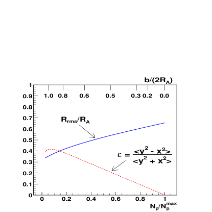
Figure 1: The derived quantities $\epsilon$ and $R_{rms}/R_{A}$, defined by Eq. 8 and 9, as a function of the number of participants relative to the maximum number. The axis on top of the graph shows the impact parameter b relative to $2R_{A}$. The curves are drawn for PbPb collisions at the SPS, but depend only slightly on the colliding system and energy.

$\epsilon$ measures the initial elliptic deformation of the overlap region and grows approximately linearly with $N_{p}$.

For the calculation presented, the entropy and therefore the number of charged particles scales as the number of participants. Recently, the experiments have reported that the charged particle multiplicity grows slightly faster than the number of participants PHENIX-Centrality ; Phobos-Centrality . This slight growth can be incorporated into hydrodynamics Kolb-Centrality , but instead the experimental $dN_{ch}/dy$ is compared directly to the model $dN_{ch}/dy$. This makes the model impact parameter slightly larger than the impact parameter determined by the experimental collaborations.

II.3 Equation of State

To solve the equations of motion, we need an Equation of State (EOS), or a relation between the pressure ($p$) and the energy and baryon densities ($e$ and $n_{B}$ respectively). In many previous hydrodynamic calculations, a bag model EOS is used Sollfrank-BigHydro ; HydroUrqmd ; HydroUrqmdHBT ; Raju-ResonanceGas . This has some advantages, since the degrees of freedom are explicit in both phases. However a typical bag model results in an EOS with a large latent heat, LH=$1-1.5\,\mbox{GeV/fm}^{3}$. Furthermore it is difficult to adjust the latent heat independently of $T_{c}$ in such models of the phase transition.

We have taken a more pragmatic approach and have constructed a thermodynamically consistent EOS with a variable latent heat in the $e$ and $n_{B}$ plane. First, note the following two derivatives which apply along the path where $n_{B}/s$ is constant

$$\left(\frac{dp}{de}\right)_{n_{B}/s} \equiv \,c_{s}^{2}$$ (10)

$$\left(\frac{ds}{de}\right)_{n_{B}/s} = \frac{s}{p+e}\,.$$ (11)

The first of these is simply the definition of the speed of sound. The second relation is surprising: it does not contain the chemical potential $\mu_{B}$ explicitly. (It follows by noting that $\left(\frac{ds}{de}\right)_{n_{B}/s}=\left(\frac{ds}{de}\right)_{n_{B}}+\left(\frac{ds}{dn_{B}}\right)_{e}\frac{n_{B}}{s}\left(\frac{ds}{de}\right)_{n_{B}/s}$ and solving for $\left(\frac{ds}{de}\right)_{n_{B}/s}$, by using thermodynamic identities). Given the speed of sound everywhere and the entropy on a single arc in the $e,n_{B}$ plane, these derivatives may be integrated to determine the entropy, s($e$,$n_{B}$). From the entropy, all other thermodynamic functions  (e.g., T and $\mu_{B}$) may be determined. Below, only the speed of sound is specified.

For smooth flows, entropy and baryon number are separately conserved. If at some initial time $n_{B}/s$ is constant everywhere in space, the two conservation laws imply that $n_{B}/s$ is constant everywhere in space $and$ time LL-Hydro . For the initial conditions specified in Sect. II.2,  $n_{B}/s=C_{n_{B}}/C_{s}$ is constant in space and remains constant as the system evolves. Therefore, the pressure is needed only along the path $n_{B}/s=C_{n_{B}}/C_{s}$. This may be directly verified by fully differentiating $\partial_{\mu}T^{\mu\nu}=0$ and noting that the derivatives of the pressure only appear as the speed of sound, $\left(\frac{dp}{de}\right)_{n_{B}/s}\equiv\,c_{s}^{2}=\left(\frac{\partial p}{\partial e}\right)_{n_{B}}+\frac{n_{B}}{e+p}\left(\frac{\partial p}{\partial n_{B}}\right)_{e}$.

Strictly speaking, transverse shock waves develop near the phase transition and invalidate the assumption of entropy conservation. However, numerical and analytical evidence has shown that entropy production in hydrodynamic simulations of nucleus-nucleus collisions is at most a few percent Ollitrault-RiemmanMixed . Below, entropy production is ignored and the pressure is specified along the trajectory $n_{B}/s=C_{n_{B}}/C_{s}$.

The EOS consists of three pieces: a hadronic phase, a mixed phase, and a QGP phase. In strong interactions, Baryon number (B), Strangeness (S), and Isospin (I) are conserved and therefore the EOS depends on $T$ and $\mu_{B},\mu_{S}$,and $\mu_{I}$. In the hadronic phase, the thermodynamic quantities –the pressure (p), the energy density ($e$), the entropy density (s), and number densities ($n_{Q}$ where Q=B,S,I)– are taken as ideal gas mixtures of the lowest SU(3) multiplets of mesons and baryons. The mix includes the pseudo-scalar meson octet ($\pi,\eta,K$) and singlet ($\eta^{\prime}$), the vector meson octet ($\rho,K^{*},\omega$) and singlet ($\phi$), the $\frac{1}{2}^{-}$ baryon and anti-baryon octets and the $\frac{3}{2}^{-}$ baryon and the anti-baryon decuplets. Specifically, $p,\,e,\,s$ and $n_{Q}$ are given by

$$n_{Q} = \sum_{i}{Q_{i}\,n_{id}^{\sigma_{i}}\,(T,\mu_{B}B_{i}+\mu_{S}S_{i}+\mu_{I}I_{i})}$$ (12)

$$p = \sum_{i}{p_{id}^{\sigma_{i}}\,(T,\mu_{B}B_{i}+\mu_{S}S_{i}+\mu_{I}I_{i})}$$ (13)

$$e = \sum_{i}{e_{id}^{\sigma_{i}}\,(T,\mu_{B}B_{i}+\mu_{S}S_{i}+\mu_{I}I_{i})}$$ (14)

$$s = \sum_{i}{s_{id}^{\sigma_{i}}\,(T,\mu_{B}B_{i}+\mu_{S}S_{i}+\mu_{I}I_{i})}\,.$$ (15)

Here the sum is over the hadrons species, $B_{i},S_{i},I_{i}$ are the quantum numbers of the i-th hadron, $\sigma_{i}$ is $+$ for bosons but $-$ for fermions, and for example, $p_{id}^{+}(T,\mu)$ is the pressure of a simple ideal Bose gas. A fast numerical method for evaluating the thermodynamic quantities of simple Bose/Fermi gases has been constructed Thermo-Pons . For a given T, $(\mu_{B},\mu_{S},\mu_{I})$ are determined by the requirements that total strangeness ($n_{S}$) and isospin($n_{I}$) be zero and that $n_{B}/s=C_{n_{B}}/C_{s}$. The thermodynamic quantities are then taken as functions of $e$ along the adiabatic path where $n_{B}/S=C_{n_{B}}/C_{s}$. This hadronic EOS is taken up to a temperature of $T_{c}=165~{}\mbox{MeV}$ or an energy density $e_{H}\approx 0.45~{}\mbox{GeV/fm}^{3}$ (see Fig. 2). The squared speed of sound is approximately 1/5 in this hadronic gas.

Above the hadronic phase, only the speed of sound squared, $c_{s}^{2}$, is specified. For the mixed phase the speed of sound was made approximately zero, $c_{s}^{2}=0.02\,c$. The width of the mixed phase (see Fig. 2) is the Latent Heat (LH), LH$=e_{Q}-e_{H}$. LH is taken as a parameter and is adjusted to form phase diagrams LH8, LH16,… with latent heats, $0.80~{}\mbox{GeV/fm}^{3}$, $1.6~{}\mbox{GeV/fm}^{3}...$ . Above the mixed phase, $e>e_{Q}$, the degrees of freedom are taken as massless and the speed of sound is accordingly, $c_{s}=\sqrt{1/3}$. We also consider two limiting cases: a Resonance Gas (RG) EOS and LH$\infty$. For a RG EOS, the speed of sound is constant above $e_{H}$. For LH$\infty$, the mixed phase continues forever ($e_{Q}=\infty$) and there is no ideal plasma phase.

With the speed of sound specified in all phases, Eq. 10 and 11 are integrated to find the pressure and entropy along the adiabatic path specified by the initial conditions, $n_{B}/s=C_{n_{B}}/C_{s}$. The full phase diagram for SPS initial conditions is shown in Fig. 2. In Sect. IV and Sect. V,

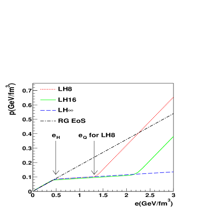
Figure 2: The pressure ($p$) versus energy density ($e$) for different EOS. EOS LH8, LH16 and LH$\infty$ become increasingly soft and have latent heats $0.8\,\mbox{GeV/fm}^{3}$, $1.6\,\mbox{GeV/fm}^{3}$, and $\infty$. The EOS are shown along the adiabatic path for SPS initial conditions, $s/n_{B}=42$. For RHIC initial conditions, $s/n_{B}=150$, the changes are small.

the subset of the EOS consistent with the available radial and elliptic flow data is found.

II.4 RQMD and the Cooper Frye Formula

Given the initial conditions and the EOS, the equations of motion are integrated in time. As the system expands and cools, the mean free path becomes much less than the nuclear radius, and the system breaks up into free-streaming particles. Typically, hydro practitioners Sollfrank-BigHydro ; Schlei-BigHydro model the breakup or $freezeout$ stage by finding a hypersurface in space and time where the temperature equals some freezeout temperature, $T=T_{f}$.

This simple picture in which all particles are emitted from a single space-time surface is however unrealistic. Different particles have different hadronic cross sections and suffer their last interaction at different times. They are emitted over a space-time region rather than on a sharp surface. Further, particles in the center rescatter for a longer time than particles in the periphery. To model this physics, the spectrum of particles $exiting$ the space-time surface is taken as the input to the hadronic cascade, RQMD Sorge-RQMD . Subsequently, the particles rescatter. Below, the space-time surface is referred to as the $switching$ surface rather than the $freezeout$ surface. The attending problems with this approach are described below after the details of the input distribution to RQMD are described.

For the family of EOS discussed above, for $T<T_{c}$, the fluid is made up of a collection of ideal gases of fermions and bosons. In order to conserve energy and momentum across the surface, the spectrum of $(\mbox{species})_{i}$ crossing the surface is given by CooperFrye ; CooperFrye-HBT ,

$$E\frac{d^{3}N_{i}}{d^{3}p} = f^{\sigma_{i}}_{id}(p\cdot U,\mu_{B}B_{i}+\mu_{S}S_{i}+\mu_{I}I_{i})$$ (16)

$$\times\,p^{\alpha}\,d\Sigma_{\alpha}$$

where $d\Sigma_{\alpha}$ is a differential element of the freezeout hypersurface and $f^{\pm}_{id}(E,\mu)$ is the Bose/Fermi distribution function $\frac{g_{J}}{\exp(\frac{E-\mu}{T})\mp 1}$. The particle index $i$ runs over all the species in the EOS – no more, no less. If the quasi-particles are interacting and the EOS is non-ideal, due to viscosity, mean fields, particle lifetimes, etc., then the $f^{\sigma_{i}}_{id}$ should be modified accordingly.

The differential elements of the hypersurface $d\Sigma_{\alpha}$ can be separated into time-like ($d\Sigma_{\alpha}d\Sigma^{\alpha}>0$) and space-like ($d\Sigma_{\alpha}d\Sigma^{\alpha}<0$) surface elements. For time-like surfaces, the integrand in Eq. 16 is positive and there is a frame (the rest frame of the surface), where $d\Sigma_{\alpha}$ = (dV,0,0,0). The spectrum of Eq. 16 is simply a thermal spectrum boosted by the flow velocity in the frame of the surface. (In practice, the surface velocity is small for most time-like surfaces). The yield of $(\mbox{species})_{i}$ leaving a surface element, $d\Sigma_{\alpha}$, is simply $n_{id}^{\sigma_{i}}(T,\mu_{B}B_{i}+\mu_{S}S_{i}+\mu_{I}I_{i})U^{\alpha}d\Sigma_{\alpha}$, as may be found by integrating the left and right sides with $\frac{d^{3}p}{E}$ and going to the rest frame of the matter.

For space-like surfaces, the integrand in Eq. 16 is both positive and negative depending on the momentum of the particle. When the integrand is positive, the particle is leaving the surface and when it is negative the particle is entering the surface. We reject particles entering the hydrodynamic surface. The distribution of particles exiting a space-like surface is

$$E\frac{d^{3}N_{i}}{d^{3}p} = f^{\sigma_{i}}_{id}(p\cdot U,\mu_{B}B_{i}+\mu_{S}S_{i}+\mu_{I}I_{i})\,$$ (17)

$$\times\,p^{\alpha}\,d\Sigma_{\alpha}\,\Theta(p^{\alpha}d\Sigma{\alpha})\,.$$

It is this distribution that we take as the input distribution for RQMD. For a discussion of the problem of space-like surfaces see Freezeout-Theta ; Freezeout-Bugaev . The number of particles leaving a differential surface element is given by a more complicated formula which is again found by integrating both sides of the equation with $\frac{d^{3}p}{E}$ Teaney-Thesis . For a stationary surface in the rest frame, the formula has the simple interpretation as the number of particles evaporating from the surface per area per unit time. A consequence of the theta-function is that energy, momentum, and particle number are not exactly conserved across the transition surface. However, the error is only $\approx 2.0\%(\approx 5.0\%)$ for central (peripheral b=8.0 fm) AuAu collisions at RHIC.

III The Space-Time Evolution

III.1 The Hydrodynamic Solution

This section reviews the hydrodynamic evolution for different EOS used in this work. The evolution at the SPS and RHIC is summarized in Fig. 3.

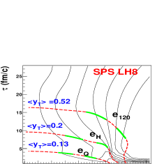
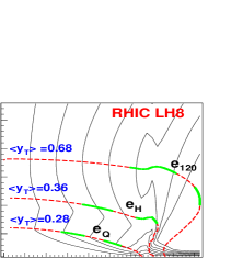
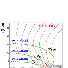
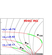
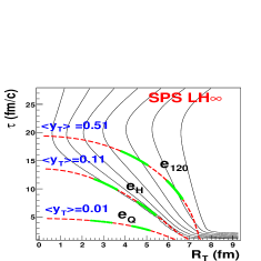
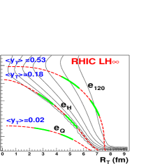
Figure 3: The left and right sides show the hydrodynamic solution at the SPS and RHIC for different EOS. The thin lines show contours of constant transverse fluid rapidity ($v_{T}=\tanh(y_{T})$) with values 0.1,0.2,…,0.7 . The thick lines show contours of constant energy density. $e_{120}$ denotes the energy density where $T=120\,\mbox{MeV}$. $e_{H}$ and $e_{Q}$ denote the energy density (for LH8) where the matter shifts from hadronic to mixed and mixed to a QGP, respectively. The shift to RQMD is made at $e_{H}$. $\langle y_{T}\rangle$ denotes the mean transverse rapidity weighted with the total entropy flowing through the energy density contours. Walking along these contours, the line is broken into segments by dashed and then solid lines. 20% of the total entropy passing through the entire arc passes through each segment.

The switching isotherm, $e_{H}$ (shown in the middle), is particularly important since in the hydro+cascade approach, the particles are injected into RQMD with the velocity distribution of this isotherm.

For EOS with a phase transition (LH8) there are three phases and three corresponding stages in the acceleration history. (i) an explosive QGP phase ($e>e_{Q}$), in which the matter accelerates rapidly, (ii) a soft mixed phase ($e_{H}<e<e_{Q}$), in which the matter free streams with constant velocity and (iii) a hadronic phase ($e<e_{H}$), in which the hadronic pressure produces additional acceleration.

The QGP phase dictates the duration and transverse size of the collision. At RHIC, the QGP pressure drives the matter outward, rapidly increasing the radius, which in turn shortens the overall lifetime. Therefore, approximately doubling the total multiplicity from the SPS to RHIC increases the total lifetime only slightly, from $10\,\mbox{fm/c}$ to $11\,\mbox{fm/c}$. All the additional multiplicity is absorbed by a slightly larger transverse radius. Similarly, for a RG EOS the acceleration is robust and continuous and increasing the total multiplicity only slightly increases the radius and lifetime. In bulk, the radii and lifetimes of RG are similar to LH8.

By contrast, for LH$\infty$, the stiff QGP phase is absent and the mixed phase is dominant at high energy densities. The strong transverse acceleration associated with LH8, is replaced with a slow evaporative process. The radius of the system slowly shrinks as a function of time. Unlike LH8, increasing the total multiplicity increases the lifetime rather than the radius. Between the SPS and RHIC the lifetime increases from from $14\,\mbox{fm/c}$ to $21\,~{}\mbox{fm/c}$. Summarizing, the QGP drives a transverse expansion; the transverse expansion increases the radius and shortens the overall lifetime compared to an EOS without the QGP push.

To quantify the input velocity distributions into RQMD, Fig. 4 plots the transverse fluid

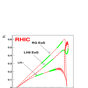
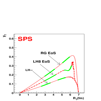
Figure 4: Walking along the $e_{H}$ contours in Fig. 3 (where the switch to RQMD is made), the transverse rapidity is traced as a function of radius at (a) the SPS and (b) RHIC for the three EOS. See Fig. 3 for an explanation of the dashed and solid segments.

rapidity versus the radius along the switching isotherm $e_{H}$ at the SPS and RHIC. For LH8 and RG, the transverse rapidity shows a linear rise with radius. A linear flow profile is often used in phenomenological fits to the particle spectra SSH-FlowProfile ; this calculation validates this approach.

For an EOS with a phase transition to the QGP (LH8), the acceleration is initially large but subsequently stalls in the mixed phase. By contrast, for an EOS without the phase transition (RG), the acceleration is robust and continuous. Therefore, although the initial transverse acceleration is smaller for a RG than for LH8, the RG velocity at the end of the SPS mixed phase is $50\%$ larger than for LH8. At RHIC, where for LH8 the QGP phase lives longer, the RG velocity is only $\approx 15\%$ larger. Although mean lifetimes and radii of the RG EOS are similar to LH8, the change in the velocity distributions from the SPS to RHIC are markedly different. Comparing LH8 to LH$\infty$ at RHIC,the LH8 flow velocity is approximately twice as large as the LH$\infty$ flow velocity.

Nevertheless, it should be noted that if freezeout is taken as $T_{f}\approx 120\,\mbox{MeV}$, then the differences between the flow velocities of the EOS is smeared out by the hadron phase, as can be seen by examining the mean flow velocities on the $e_{120}$ curves in Fig. 3. Indeed, the hadronic phase of LH$\infty$ (which lives longer, since it is born with no transverse velocity) can partially compensate for the weak initial acceleration. Along the $T_{f}\approx 120\,\mbox{MeV}$ isotherm, the flow velocities of LH$\infty$, RG and LH8 are roughly comparable.

To characterize the flow in non-central collisions for the EOS used in this work, we follow Kolb $et$ $al.$ Kolb-UU and calculate a quantity derived from the stress tensor for

$$\epsilon_{p} \equiv \frac{\left\langle T^{xx}-T^{yy}\right\rangle_{S}}{\left\langle T^{xx}+T^{yy}\right\rangle_{S}}\,,$$ (18)

where the $\langle\rangle_{S}$ denotes an average over the transverse plane weighted with the entropy per area per unit spatial rapidity, $s\gamma\,\tau dx\,dy$. $\epsilon_{p}$ is related to $\frac{\left\langle p_{x}^{2}-p_{y}^{2}\right\rangle}{\left\langle p_{x}^{2}+p_{y}^{2}\right\rangle},$ the final momentum anisotropy of the particle distribution Ollitrault-Elliptic which ultimately is related to $v_{2}(p_{T})$ Kolb-Flow .

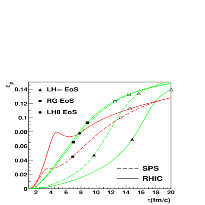
Figure 5: Following Kolb $et$ $al.$ Kolb-UU , we show the anisotropy of the stress tensor, $\epsilon_{p}$ (a measure of elliptic flow) for the EOS used in this work. The solid (dashed) curves are for RHIC (SPS). The solid (open) symbols indicate when the center of the fluid passes through a temperature of 160 MeV (120 MeV). The solid symbols are therefore representative of the switching temperature to RQMD or $e_{H}$ in Fig. 3.

The general trends seen in $\epsilon_{p}$ follow from the discussion above on the hydrodynamic response of each EOS. LH8 shows a strong early response followed by a stall and subsequent flattening as the matter distribution becomes almost spherical. At RHIC the strong early response lives substantially longer as the matter spends a larger fraction of its total lifetime in the QGP phase. For LH$\infty$ the matter is initially stalled but rapidly accelerates as it slowly enters the hadronic phase (see Fig. 3 (e) and (f)).

III.2 Qualitative Predictions of the Hydrodynamic Response

We can now make some qualitative predictions from the hydrodynamic solution. Assume momentarily that the final hadron momentum distributions reflect the boundary between the mixed and hadronic phases or $e_{H}$ in Fig. 3. Then with the curves presented in the last section, LH8 predicts two qualitative changes. First with Fig. 5, between the SPS and RHIC, $p_{T}^{2}$ weighted elliptic flow should increase by almost a factor of two as the QGP replaces the mixed phase and dominates the early evolution. Second with Fig. 4, the total transverse momentum should increase by 30% as the QGP drives additional transverse motion. The flow differentiates LH8 from a RG EOS and from LH$\infty$. Since RG EOS accelerates continuously and does not stall in the mixed phase, the transverse momentum is larger at both the SPS and RHIC. In addition, for SPS collision energies, the elliptic flow ($\epsilon_{p}$) for a RG EOS is almost a factor of two larger than for LH8. For LH$\infty$, the transverse momentum is very low until the very end.

To make these qualitative predictions quantitative and to compare the hydrodynamic solution to experimental data, it is essential to model hadronic freezeout. Between the time when $T_{f}=160\,\mbox{MeV}$ (the solid symbols) and $T_{f}=120\,\mbox{MeV}$ (the open symbols) elliptic flow changes dramatically for each EOS. This is especially true for LH8 at the SPS, where the mixed phase abruptly stalls the development of elliptic flow but then the hadronic phase rapidly completes the development. The differences in the early acceleration tend to get washed out by the hadronic stage. Indeed, even LH$\infty$ has a reasonable radial and elliptic flow by $T_{f}=120\,\mbox{MeV}$. The extent to which signatures of the early QGP acceleration remain in the final spectra depends on whether the freezeout temperature should be taken as $T_{f}=120\,\mbox{MeV}$ or $T_{f}=160\,\mbox{MeV}$. The breakup of a heavy ion collision can only be addressed with hadronic cross sections and expansion rates.

III.3 RQMD – Input and Response

Relativistic Quantum Molecular Dynamics (RQMD) Sorge-RQMD is a hadronic transport computer code which incorporates many known hadronic cross sections. RQMD has been used extensively to model the heavy ion dynamics Sorge-Strange ; Sorge-elliptic ; Sorge-PreEquilibrium ; Sorge-kink ; Sorge-Time . Briefly, when two particles come within $d<\sqrt{\sigma/\pi}$, they elastically scatter or form a resonance. Resonance formation and decay dominate the evolution. The principal reactions are $\pi\pi\rightarrow\rho$, $\pi\,N\rightarrow\Delta$, $\pi\,K\rightarrow K^{*}$, and $\pi\,\Lambda\rightarrow\Sigma^{*}$. Only binary collisions are considered in this hadron cascade. Before discussing the response of RQMD, we first consider the input.

The time distributions are found by projecting the entropy distribution on the switching isotherm $e_{H}$ in Fig. 3 (or $T=160\,\mbox{MeV}$) onto the $\tau$ axis. In Fig. 6

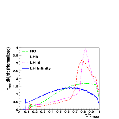
Figure 6: The fraction of pions emitted into RQMD per unit of time relative to the last instant($\tau_{max}$) that the matter is evolved by hydrodynamics.

the fraction of pions (or entropy) injected into RQMD per unit $\tau$ is plotted as a function $\tau/\tau_{max}$ for each EOS. For LH8, very few particles are evaporated from space-like surfaces at early times, and at $\tau/\tau_{max}\approx 0.8$ ($\tau\approx 9\,\mbox{fm/c}$) particles are emitted in bulk from the time component of the switching surface. For LH$\infty$, particles are continuously evaporated from the transition surface and the radius slowly decreases. Therefore, the time distribution is relatively uniform. Finally for a RG EOS, the freezeout surface is not box-like and particles are also emitted into RQMD slowly and continuously.

Now consider the dynamic response of the hadronic cascade. For LH8, the hydrodynamic input into RQMD can be characterized as a simple thermal model with a linearly rising flow profile with a uniform radial distribution except at the edge of the distribution where there is a small maximum. Once this input distribution is taken, the hadrons re-scatter within RQMD and different particles decouple from the cascade at different times. Fig. 7 (a) plots the

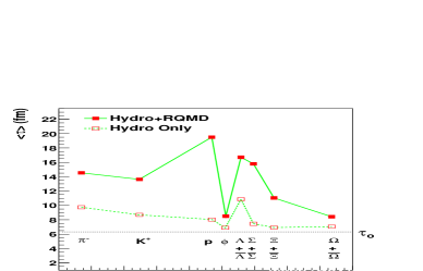
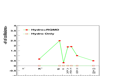
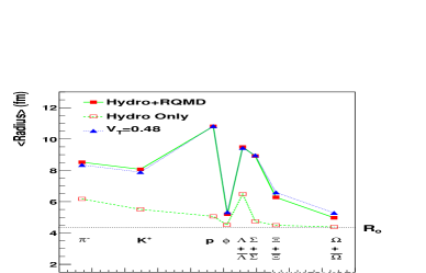
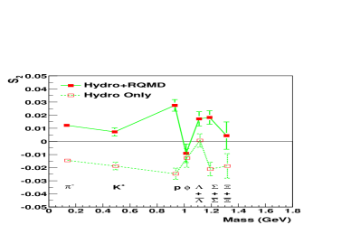
Figure 7: The mean (a) emission time, (b) number of collisions, (c) emission radius, and (d) spatial anisotropy $s_{2}$ (see Eq. 20) as a function of particle mass with and without the RQMD hadronic after-burner. The averages are taken over the points of last interaction for AuAu collisions at b=6 fm at RHIC. In (a) and (c), $\tau_{o}$, and $R_{o}$ label the mean emission time and radius of the $\phi$ meson. $v_{T}$ denotes the freezeout drift velocity of Eq. 19.

mean emission time $<\tau>$ (the time of last interaction) versus the mass of the particle species. Also shown is $<\tau>$, when all collisions in RQMD are switched off and only resonance decays are allowed. The mean number of collisions experienced by a particle is shown in Fig. 7 (b). The mesons scatter approximately once after their principal resonances ($\rho,\,K^{*},$ etc.) decay and decouple around $\tau\approx 14\,\mbox{fm/c}$. In contrast, due to strong meson-baryon resonances $\Delta,~{}\Sigma^{*},...$ , nucleons and hyperons ($\Lambda$ and $\Sigma$) scatter approximately twice and decouple around $\tau\approx 18\,\mbox{fm/c}$. The $\phi$ and $\Omega^{-}$ are emitted directly from the phase boundary since they have small hadronic cross sections.

The duration of the hadronic stage dictates the spatial extent of the final source. In Fig 7 (c), the mean radius is shown as a function of particle mass with and without re-scattering in the hadronic cascade. For comparison, we apply the simple formulas: We assume all particles are emitted from the switching surface at a mean radius $R_{o}$ and a mean time $\tau_{o}$, with a constant radial velocity $v_{T}$ (see Fig. 7 (a) and (c)). Since $\phi$ is emitted directly from the switching surface, $R_{o}$ =$\langle R_{\phi}\rangle$ and $\tau_{o}=\langle\tau_{\phi}\rangle$. With the formula distance = velocity $\times$ time, we have

$$\langle R\rangle_{x}=R_{o}+v_{T}(\langle\tau_{x}\rangle-\tau_{o}),$$ (19)

where $\langle R\rangle_{x}$ ($\tau_{x}$) is the freezeout radius (time) of particle x and $v_{T}$ is the freezeout drift velocity. This velocity incorporates a thermal drift velocity and the flow velocity of the source. Given a constant velocity as a function of mass $v_{T}\approx.42\,c$, a very simple fit to the freezeout radii is obtained, as shown in Fig. 7(c). Thus, hadronic cross sections dictate the final freezeout radii of the source.

Hadronic cross-sections also dictate the spatial geometry in non-central collisions. In non-central collisions the ellipticity of the source at freezeout is quantified by the spatial anisotropy,

$$s_{2}=\left\langle\frac{x^{2}-y^{2}}{x^{2}+y^{2}}\right\rangle\,.$$ (20)

Here, the averages are taken over points of last interaction in the cascade. $s_{2}$ is negative for the initial almond-shaped distribution but positive for a cucumber-shaped distribution. Fig. 7(d) shows $s_{2}$ without re-scattering but with resonance decays (Hydro Only) and with hadronic re-scattering (Hydro+RQMD). The initial elliptic flow ($v_{2}$) changes the overall geometry ($s_{2}$) by the end of the RQMD stage. At the end of the hydrodynamic stage $s_{2}$ is negative, indicating that the source retains at least some of its initial almond distribution. $s_{2}$ becomes positive as the system evolves and the momentum asymmetry changes the source geometry. For nucleons, $s_{2}$ is almost +3% for modest impact parameters; this may have observable consequences STAR-EllipticParticle .

III.4 Impact Parameter Dependence of the Space Time Evolution

In the previous section, we discussed how hadronic cross sections control the lifetime and geometry of the final hadronic distributions. Now the impact parameter is varied and the freezeout distributions are modified. In non-central collisions, the number of charged particles scales as the number of participants; therefore the lifetime of the hadronic stage should also scale as the number of participants. However, the hadronic lifetime is also a function of the cross section, the radius, and the expansion rate ($\partial_{\mu}U^{\mu}$). These depend respectively on the particle species, the r.m.s. radius of the initial geometry, and the EOS. In Fig. 8, the different contributions

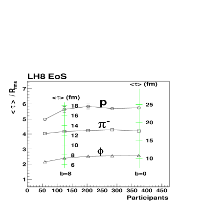
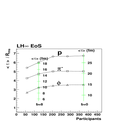
Figure 8: The mean emission time $\langle\tau\rangle$ relative to the Glauber r.m.s. radius (see Eq. 8) as a function of the number of participating nucleons for (a) LH8 and (b) LH$\infty$. The free axes show the absolute lifetime at impact parameters b=0 fm and b=8 fm.

to the total lifetime are studied. We plot the mean emission time $<\tau>$, divided by size $R_{rms}^{Glauber}$, as a function of the number of participants for different particles and EOS. To set the absolute scale, the “free” axes show $<\tau>$ directly at two impact parameters.

Consider first the LH8 curves (a): The total lifetime for all particle species falls by approximately 30% from central (b=0 fm) to peripheral (b=8 fm) collisions. The order of particle emission remains as the impact parameter is varied: First rare species ($\phi,\Omega$) are emitted, then mesons ($\pi,K$) and finally baryons ($N,\Lambda$). For the $\phi$, which is representative of the hydrodynamic stage, the curves in Fig. 8(a) are flat at the 15% level, indicating that the total lifetime scales roughly with the size of the overlap region. For pions, the total lifetime also scales with $R_{rms}$. For protons, indicative of baryon emission, the total lifetime does not quite scale as $R_{rms}$ but rather depends on the absolute number of charged particles in addition to the geometry. This is natural since the freezeout of protons is controlled by the formation of $\Delta$ resonances.

For LH$\infty$, $\langle\tau\rangle/R_{rms}$ does change more rapidly than for LH8 This is especially true for nucleons. However, for $\phi$ and $\pi$ the difference in the $N_{p}$ dependence of $\langle\tau\rangle/R_{rms}$ is small and to a reasonable approximation, the lifetimes of $\phi$ and $\pi$ scale with $R_{rms}^{Glauber}$ for all EOS. Changing the EOS simply moves the various curves up and down on Fig. 8 (a) and (b). A RG EOS was also studied (not shown) and the lifetime and $N_{p}$ dependence were quite similar to LH8.

Eq. 19 relates the freezeout radii and geometry of the different particles to a freezeout time and a single freezeout drift velocity ($v_{T}$) and a single freezeout radius ($R_{\phi}$). This simple formula was found to be applicable to all impact parameters with approximately the same drift velocity as in central collisions. The lifetimes and radii ($R_{\phi}$) all scale with the root mean square radius.

Given the rather simple scaling of lifetimes and radii as a function of impact parameter, it is natural to consider the density of pions at freezeout as first done in HydroUrqmd . Since pion number is approximately conserved during the cascading process, we have $s\propto n_{\pi}$ and the freezeout entropy density is

$$\frac{dN_{\pi}/dy}{\pi<\tau><R>^{2}}\sim s_{f}\,.$$ (21)

This quantity is shown as a function of the number of participants for RHIC collisions in Fig. 9.

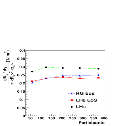
Figure 9: The density of pions at freezeout (see text) versus the number of participants for different EOS. Here $<\tau_{\pi}>$ and $<R_{\pi}>$ denote the mean pion emission time and radius.

The freezeout entropy density is roughly constant as a function of impact parameter. In addition, the freezeout density is independent of EOS in spite of differences in transverse velocity gradients. It has been argued that central PbPb collisions cool to a lower temperature than peripheral collisions since transverse and longitudinal velocity gradients are larger in peripheral collisions Hung-Freezeout . However at least in the model, freezeout is not driven by the expansion rate; rather, the freezeout condition reflects a density where the mean free path becomes comparable to the radius of the nucleus.

Next we hold the collision geometry fixed and examine the changes in lifetime, radius and freezeout density as the initial entropy density ($i.e.$, the collision multiplicity) is increased. Fig. 10 (a) and (b) shows the lifetime and emission

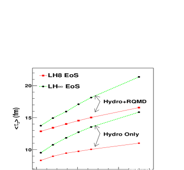
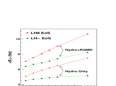
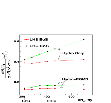
Figure 10: The mean pion (a) emission time, (b) emission radius, and (c) freezeout density as a function of the total multiplicity in a PbPb collision at b=6 fm. The SPS and RHIC arrows denote where the charged particle per participant per rapidity matches SPS and RHIC initial conditions respectively.

radius for a PbPb collision at b=6 fm as the multiplicity per participant is increased from the SPS to the RHIC domain. For LH8, the radius increases but the emission time does not, while for LH$\infty$ the situation is exactly reversed.

This behavior is readily understood as entropy conservation in the transverse plane. Entropy conservation (see Eq. 4) relates the entropy density to the Bjorken time ($\tau$), the total conserved entropy per unit rapidity ($dS_{tot}/dy$), and the effective area ($A_{eff}$) of the source with the schematic relation,

$$<s>\sim\frac{dS_{tot}/dy}{\tau A_{eff}(\tau)}.$$ (22)

As seen with Fig. 10(c), the entropy density at freezeout ($s_{f}$) is roughly constant as a function of beam energy. The freezeout time $\tau_{f}$ may therefore be related to freezeout entropy density $s_{f}$ with

$$\tau_{f}\sim\frac{dS_{tot}/dy}{s_{f}A_{eff}(\tau_{f})}\,.$$ (23)

For LH8, the strong transverse acceleration rapidly increases the area and lowers the entropy density $s$ to $s_{f}$. Consequently, as the multiplicity is doubled, the total lifetime increases by only 20%. For LH$\infty$, the radius does not increase but the lifetime increases significantly. Thus the transverse expansion, together with entropy conservation, ultimately determine the total lifetime.

IV Radial Flow From the SPS to RHIC

IV.1 The SPS

In a traditional hydrodynamic calculation Sollfrank-BigHydro ; Schlei-BigHydro ; Kolb-Flow , the pion and nucleon yields fix the total entropy and baryon number in the initial conditions. The freezeout temperature is adjusted to fit the pion and proton $p_{T}$ spectra. In the hydro+cascade approach advocated here, the freezeout temperature is not a parameter since particles decouple from the cascade when their collision rates become small. Therefore, the pion and nucleon yields set the total entropy and baryon number as before, but the slope parameters provide significant information about the EOS. In particular, the latent heat of the phase transition which best matches the pion and nucleon $p_{T}$ spectrum is $\mbox{LH}\approx 0.8\,\mbox{GeV/fm}^{3}$.

In the previous section, we discussed a family of EOS, each with a different latent heat. Now we show in Fig. 11,

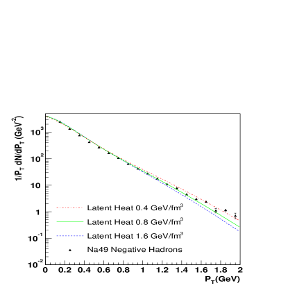
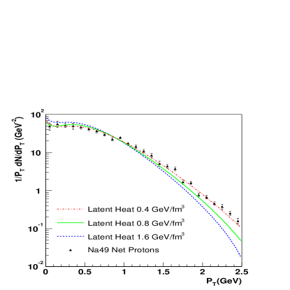
Figure 11: A comparison to NA49 NA49-Spectra (a) negative hadron and (b) net-proton spectra for different EOS.

the calculated net proton spectrum for the resonance gas EOS and for EOS LH4-LH16. The experimental and theoretical spectra are absolutely normalized. The two numbers parameterizing the initial conditions $C_{S}$ and $C_{n_{B}}$ (see Table 1) are adjusted to match the height of these spectra. The model curves have been multiplied by a factor of 0.93 to account for the fact that the data is 5% central. Once the height of the spectrum is tuned, the shape of the spectrum is determined by the course of the hydrodynamic evolution, or more generally, by pressure gradients and the duration of the collision. Therefore, it is significant that hydrodynamics generates a flow $v_{T}\approx 0.5$, which is needed to explain the spectra. This flow velocity was extracted from a variety of thermal analyses Uli-Expand .

For EOS with large latent heats (e.g. LH16), the $p_{T}$ spectrum is too soft. This is because the hydrodynamic system spends a long time in the mixed phase in which pressure gradients do not generate collective motion. Bag-model equations of state, employed in many hydrodynamic calculations Sollfrank-BigHydro ; HydroUrqmd , typically have a latent heat from $1-1.5\,\mbox{GeV/fm}^{3}$ which makes the EOS rather soft. This large latent heat is usually compensated by adjusting the freezeout temperature Sollfrank-BigHydro . An EOS with a modest first order phase transition (e.g. LH4 and LH8) generally reproduces the shape of the $p_{T}$ spectra in Fig 11. Unfortunately, a RG EOS can also reproduce the shape of the $p_{T}$ spectrum and additional experimental information is needed to separate EOS.

The slope systematics of $\Lambda$, $\Xi$ and $\Omega$ provide the necessary information. The presence of a phase transition stalls the acceleration Rischke-Lifetime ; HS-soft ; therefore information about the velocity at the end of the mixed phase can separate a RG EOS from LH8. At the SPS, the spectra of the different particle species are all reasonably exponential and a slope parameter, $T_{slope}$ is extracted. Specifically the data are fit to the following form,

$$\frac{1}{M_{T}}\frac{dN}{dM_{T}} = C\exp(-\frac{M_{T}}{T_{slope}}),$$ (24)

where $M_{T}=\sqrt{m^{2}+p_{T}^{2}}$. In this parameterization, the slope parameter $T_{slope}$, is directly related to the $<M_{T}>=2T_{slope}+\frac{m^{2}}{T_{slope}+m}$. The model spectra are fit with Eq. 24 over the range corresponding to the WA97 WA97-Slopes experimental acceptance ($M_{T}-m=0.0-0.9\,\mbox{GeV}$); the slope parameters are shown versus particle mass with and without RQMD in Fig. 12(a).

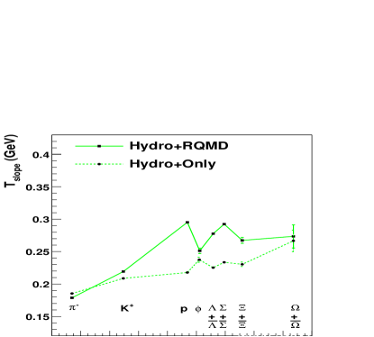
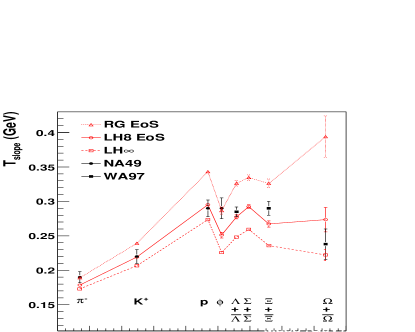
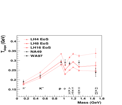
Figure 12: A compilation of slope parameters from the SPS experiments and a comparison to the model for different EOS. (a) shows the model slope parameters with and without hadronic rescattering (b) shows the slope parameters for three qualitatively different EOS: RG, LH8, and LH$\infty$. (c) shows the sensitivity to the latent heat in the LH family of EOS. NA49 data points are from NA49-Slopes while WA97 data points are from WA97-Slopes . The model spectra are fit with Eq. 24 over the range corresponding to the WA97 WA97-Slopes experimental acceptance ($M_{T}-m=0.0-0.9\,\mbox{GeV}$).

First look at the “Hydro Only” curves. The slopes increase approximately linearly with mass as is expected in a thermal expanding source model SZ-FlowProfile ; SSH-FlowProfile ; SR-FlowProfile . The non-monotonous increasing mass in the “Hydro Only” curves is due to resonance decays and the baryon content of the particles. Once RQMD is included, the slopes are modified by hadronic rescattering leading to mass dependence characteristic of differential freezeout Sorge-Strange . Note the following features. First, in the model the $\Omega$ gives a good measure of the flow velocity at the end of the mixed phase. Second, note the $\approx 40\%$ increase in the nucleon and $\Lambda$ slope parameters and the small $decrease$ in the pion slope parameter, due to cooling. As the hadron gas expands, the pions excite $\Delta$ and $\Sigma^{*}$ resonances and drive additional transverse motion in the nucleon and hyperon sectors. However, the pions increase the nucleon $\langle M_{T}\rangle$ only at the expense of their own kinetic energy. In a traditional hydrodynamic approach, the hydrodynamic evolution would be continued to match the slope of the nucleon spectrum. Judging from Fig. 12(a), this is misguided, as a nucleon receives much of its momentum after pions have decoupled. As shown below, the nucleon receives about 20% of its transverse kinetic energy from the pion “wind”, irrespective of the colliding energy. To incorporate the rich freezeout dynamics of a cascade, different freezeout temperatures and velocities should be taken for different particles Hung-Freezeout .

A comparison to the available data on slope systematics is given in Fig. 12: (b) shows the slopes for different types of EOS while (c) shows the sensitivity to the latent heat. Although RG and LH4 are capable of reproducing the pion and nucleon spectra, they significantly over-predict the slope parameters of $\Lambda$, $\Xi$ and $\Omega^{-}$. This is because LH4 and RG already have developed a substantial flow velocity at the end of the mixed phase. The slope parameter of the $\Omega$ is a sensitive measure of the flow velocity at the end of the mixed phase since the flow velocity is amplified by the mass in the approximate formula $T_{slope}=T_{th}+m\,<v>^{2}$. LH$\infty$, by contrast, under-predicts the slope parameters of $\Lambda$ and $\Xi$, indicating that $\langle\mbox{v}_{T}\rangle$ is too small at the end of the mixed phase. With LH8, the acceleration is modest – but significant – and the slope systematics are generally reproduced. In the model, only an EOS which has both a stiff and soft piece is capable of reproducing general trends seen in the particle spectra.

IV.2 Qualitative Changes at RHIC

It was argued above that LH8 provides the best description of the radial flow at SPS: Now the same EOS is used to make predictions for RHIC. At RHIC, the initial energy density is well above the phase transition, and the large early pressure is expected to drive collective motion. In Fig. 13, the nucleon

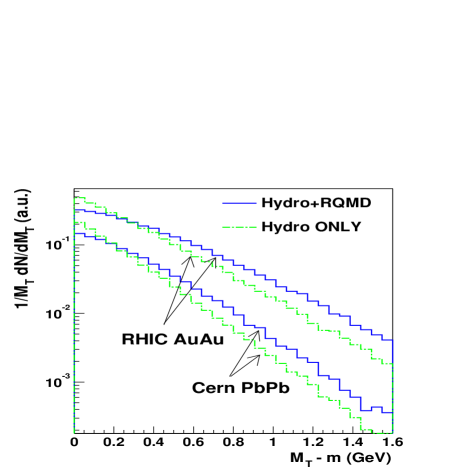
Figure 13: The nucleon $M_{T}$ spectrum at the SPS and RHIC with and without the RQMD after-burner.

$M_{T}$ spectrum for the SPS and RHIC are shown with and without the hadronic rescattering in RQMD. Two features are immediately observed: 1. The $\langle M_{T}\rangle$ increases as the collision energy is increased from the SPS to RHIC Kataja-MixedPhase ; HydroUrqmd ; Ollitrault-MixedPhase . 2. The spectra without hadronic rescattering are reasonably well described by a single exponential ($i.e.,$ they look linear on the log plot shown). Once rescattering is included the spectra are curved; this curvature grows from the SPS to RHIC. Describing the spectra with a single slope parameter, although useful in summarizing a large variety of data, is only approximate.

IV.3 The $\langle M_{T}\rangle$ from the SPS to RHIC and Beyond

To summarize the bulk energy transport in the model we show in Fig. 14:

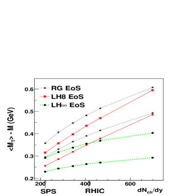
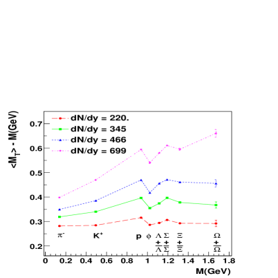
Figure 14: For PbPb collisions at b=6 fm, (a) shows $\langle M_{T}\rangle-M$ for nucleons versus the charged particle multiplicity ($dN_{ch}/dy$). For each EOS the upper curve is with hadronic rescattering (Hydro+RQMD) and the lower curve is without hadronic rescattering (Hydro Only). (b) shows $\langle M_{T}\rangle-M$ for different particle species as the total multiplicity is increased from the SPS to RHIC and beyond.

(a) the $\langle M_{T}\rangle-M$ for nucleons as a function of collision energy ($dN_{ch}/dy$) for different EOS, and (b) the $\langle M_{T}\rangle-M$ for different particle species as a function of mass for different collision energies (particle multiplicities).

Fig. 14(a) demonstrates that the additional entropy gets converted into additional transverse motion for each EOS. For each EOS, the hadronic contribution to the mean $\langle M_{T}\rangle$ remains constant and is approximately 20% for LH8 and RG, but is approximately 30% for LH$\infty$. LH$\infty$ is a special case, and we may say that the RQMD contribution is approximately 20% and is independent of the underlying EOS.

Fig. 14(b) demonstrates how the increase in the mean $M_{T}$ influences the spectra of different particles by plotting $\langle M_{T}\rangle$ versus mass Sorge-Strange . At the SPS the flow velocity at the end of the mixed phase is relatively small – $v_{T}\approx 0.4$ . The slopes before the RQMD phase show a linear rise characteristic of hydro, $T_{slope}=T_{th}+m\,\langle v^{2}\rangle$. When the flow velocity is small, hadronic rescattering changes the linear mass dependence significantly, giving the characteristic shape observed at the SPS. As the flow velocity increases from the SPS to RHIC and beyond, the linear rise with mass becomes increasingly steep and hadronic rescattering, while still contributing to 20% of the $\langle M_{T}\rangle$ for nucleons, does not change the overall mass dependence. The qualitative shape of the mass dependence of $\langle M_{T}\rangle$ therefore gives a good measure of the flow velocity at the end of the mixed phase. Since this flow velocity is different for different EOS, the mass dependence of the $\langle M_{T}\rangle$ can therefore separate the different EOS studied.

IV.4 The Flow Profile from the SPS to RHIC

The curvature in the $M_{T}$ spectrum is a signature of a radially flowing thermal source. The general features can be understood from a simple thermal model. For a cylindrically symmetric shell, which expands longitudinally in a boost invariant fashion and which freezes out in an instant with constant temperature T, and a radial velocity $v_{T}=\tanh{\rho}$, the $M_{T}$ spectrum is given by SZ-FlowProfile ; SSH-FlowProfile ; SR-FlowProfile

$$\frac{1}{M_{T}}\frac{dN}{dM_{T}} \propto M_{T}I_{0}\left(\frac{M_{T}\sinh\rho}{T_{th}}\right)K_{1}\left(\frac{M_{T}\cosh\rho}{T_{th}}\right)\,.$$

For $p_{T}\gg m$ we have

$$T_{slope} = T_{th}\sqrt{\frac{1+v}{1-v}}$$ (26)

Generally, increasing the velocity increases the curvature of the final spectrum for heavy particles. Increasing the mass also increases the curvature of the flow profile. The shape of the spectrum, together with the mass dependence of the observed particle, may provide a good experimental measure of the velocity of the source at hadronization.

Hadronic rescattering changes the curvature seen in the thermal spectra discussed above. First, different particle types have different hadronic cross sections and therefore freezeout at different times and with different velocities. The curvatures in the final spectra measure these different freezeout velocities. Second, the cascade generates additional transverse flow predominantly in the low $M_{T}$ region of the spectra. To quantify these effects, we divide the $M_{T}$ spectra into a low $M_{T}$ region, $0<M_{T}<0.6\,\mbox{GeV}$ and a high $M_{T}$ region, $0.6\,\mbox{GeV}\,<M_{T}<1.6\,\mbox{GeV}$. We then fit an exponential in both domains. Thus, there is a low $M_{T}$ slope and high $M_{T}$ slope. We have checked that this parameterization gives a good description of the shape for all the spectra considered. Fig. 15 shows the low

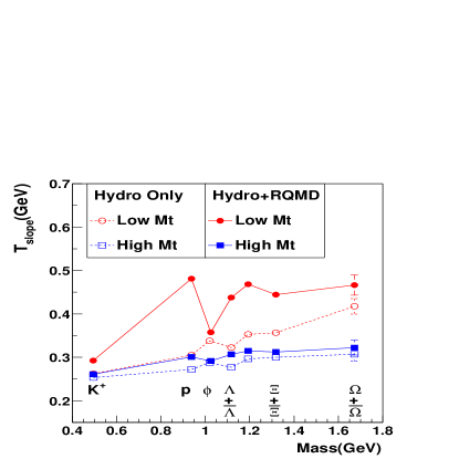
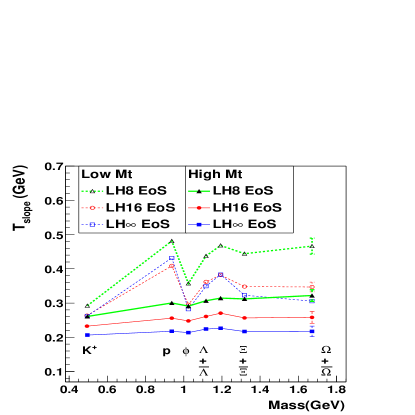
Figure 15: Each particle spectrum in central AuAu collisions, $\frac{dN}{M_{T}\,dM_{T}}$, is fit with an exponential slope parameter from $0<M_{T}<0.6\,\mbox{GeV}$ and from $0.6<M_{T}<1.6\,\mbox{GeV}$. Thus there is a low and a high $M_{T}$ slope representative of the slopes measured by the STAR STAR-Spectra and PHENIX collaborations PHENIX-Spectra . (a) shows the mass dependence of the low and high $M_{T}$ slopes with and without the RQMD after-burner for LH8. (b) shows the mass dependence of the low and high $M_{T}$ slopes for the different EOS with the RQMD after burner.

and high $M_{T}$ slopes as a function of the particle mass, with and without the RQMD after-burner. The curves illustrate the collective acceleration which occurs during hadronic rescattering, and illustrate an interplay between freezeout and hydrodynamic behavior. First look at the “Hydro Only” curves: the curvature (i.e. the difference between the low $M_{T}$ and the high $M_{T}$ slopes) increases with mass as expected from Eq. IV.4. When the cascade is included, rescattering changes this mass dependence. The curvature no longer increases but remains approximately constant after the nucleon mass. It is useful to compare the flow of the nucleon and the $\Omega^{-}$. The nucleon has a smaller mass which, according to Eq. IV.4, decreases the curvature relative to the $\Omega^{-}$. However, the nucleon decouples later than the $\Omega^{-}$ and through hadronic rescattering develops larger transverse velocity,  which increases the curvature. In the end, the $\Omega^{-}$ and the nucleon have approximately the same spectral shape. In contrast, the $\phi$, which has approximately the same mass as the nucleon but which decouples early, has very little spectral curvature. To summarize, an interplay between the differential freezeout dynamics and the curved thermal spectra of Eq. IV.4 results in rich features in the final spectra of different particles.

Before discussing their impact parameter dependence of these rich features (see Sect. IV.6), we study the sensitivity of the spectra to the EOS. The mass dependence of the slopes is a feature of an expanding thermal source and differential freezeout. It is not a feature of the underlying EOS. In Fig. 15, the low $M_{T}$ and high $M_{T}$ slopes are shown for three different EOS. For this discussion, the direct comparison of model and data nucleon spectra in Fig. 18 may be helpful. For the high $M_{T}$ slopes for all particles, there is a simple ordering, $T_{slope}^{LH8}>T_{slope}^{LH16}>T_{slope}^{LH\infty}$, which reflects (through Eq. 26) the ordering of the transverse flow, $v_{T}^{LH8}>v_{T}^{LH16}>v_{T}^{LH\infty}$. In the low $M_{T}$ region, the ordering is more complex and reflects the space-time structure of the freezeout surface for different EOS. LH$\infty$ evaporates particles shrinking radially inward. This causes an enhancement of the particle yield at low $M_{T}$ and gives LH$\infty$ a significant slope in the low $M_{T}$ region. Still, with LH8 the $\Omega{-}$ shows much more flow at low $M_{T}$ than it does with LH16 and LH$\infty$ indicating a large velocity at the end of the mixed phase.

The curvature in the $M_{T}$ spectra at small $M_{T}$ is a consequence of the mass dependence of Eq. IV.4 and hadronic rescattering, as discussed above. Now the role of hadronic rescattering, or the “pion wind”, is studied in detail with Fig. 16.

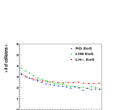
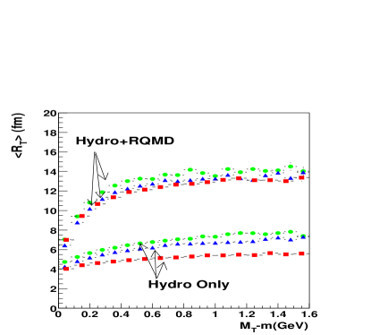
Figure 16: For nucleons in central AuAu collisions, (a) analyzes the number of collisions experienced by a nucleon as function of $M_{T}$ while (b) analyzes the mean freezeout radius of a nucleon as a function of $M_{T}$.

At low $M_{T}$, where the cascade is most effective, all the nucleons come from the center of the nucleus, as can be seen in Fig. 16(b). Accordingly, the number of collisions is larger and the nucleons are accelerated more. At high $M_{T}$, the nucleon spectrum (recall Fig. 13) is simply shifted with 2-3 collisions by a constant amount, approximately $300\,\mbox{MeV}$, which increases the slope. These collisions happen over a time scale of $\approx 10\,\mbox{fm}$ and the collision rate is therefore $\approx\frac{1}{5\,\mbox{fm}}$. Collecting these observations, nucleons coming from the center of the collision freezeout last, populate the low $M_{T}$ region, and are kicked the most by the pion wind.

IV.5 Comparison to Central RHIC Data

Now we compare model predictions to the first RHIC spectra. Keep in mind the two major predictions of hydrodynamics introduced in Sect. IV.2. First, $<M_{T}>$ should increase significantly. Since LH8 was found to give the best agreement to SPS flow data, LH8 should give the best agreement at RHIC. Out of all the EOS studied, the flow velocity increases the most for LH8. Second, the spectra should show the flow profile of Eq. IV.4. This profile is sensitive to the particle mass and flow velocity. At RHIC therefore, LH8 predicts a significant change in slope from low $M_{T}$ to high $M_{T}$.

Fig. 17 and Fig. 18 show the absolutely normalized

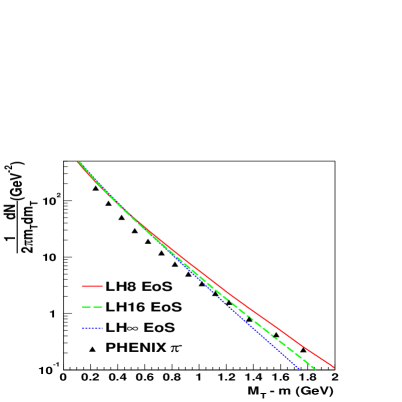
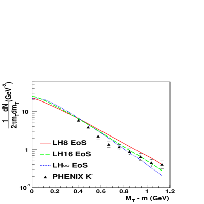
Figure 17: A comparison to PHENIX spectra PHENIX-Spectra : (a) compares $\pi^{-}$ spectra. (b) compares $K^{-}$ spectra. Both the model and the experimental spectra are absolutely normalized.

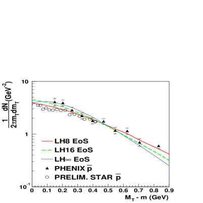
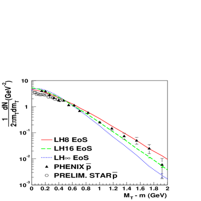
Figure 18: A comparison to PHENIX PHENIX-Spectra and STAR STAR-Spectra $\bar{p}$ spectra for (a) low and (b) high $M_{T}$, respectively. Both the model and the experimental spectra are absolutely normalized.

model spectra for three different EOS compared to data for $\pi^{-}$,$K^{-}$ and $\bar{p}$. For each particle type, the transverse mass spectrum is strong. Generally, LH$\infty$ under-predicts the flow profile while LH8 reproduces the spectrum. The data indicate a strong macroscopic transverse response, as expected of an EOS with speed of sound $c_{s}^{2}\approx 1/3$. Some caveats must be mentioned. It is known that the transverse mass spectrum is sensitive to the details of the initial profile and longitudinal expansion Sollfrank-BigHydro . In particular, the transverse mass spectrum is modified if the initial entropy density is distributed according to binary collisions Kolb-Centrality . However, even when the entropy is distributed entirely according to binary collisions, the change in the spectrum is small. The strong increase in radial flow from the SPS to RHIC is reproduced by the hydrodynamic response of LH8. Thus, prediction (1) is borne out by the first spectra at RHIC. Next, look at the shape of the $\bar{p}$ spectrum in Fig 18. This flattening at low $M_{T}$ is characteristic of a flow profile. We expect a smaller flattening in the kaon spectrum. Thus, the rich flow profile of Eq. IV.4 is also borne out in the first RHIC data and prediction (2) is correct.

It is worthwhile to plot the $\pi^{-}$ and $\bar{p}$ spectra on the same plot. The spectra almost cross for $p_{T}\approx 2.3\,\mbox{GeV}$ It was recently pointed out that the measured $\pi^{-}/\bar{p}$ ratio is several times above the expected ratio from jet fragmentation and from a hydrodynamic calculation that does not incorporate chemical freezeout Vitev-Baryon . The ratio is readily explained in a simple hydro/thermal model with additional hadronic scattering. The thermal input into RQMD is roughly summarized by Eq. IV.4. Above $M_{T}>2.0\,\mbox{GeV}$ without rescattering, the slope parameters of pions and nucleons approach the universal value $T_{slope}\approx 250\,\mbox{MeV}$. This slope is given by Eq. 26 with the parameters for $T_{th}=160\,\mbox{MeV}$ and $v_{T}=0.45\,c$. Accounting for hadronic rescattering, the nucleon slope at large $p_{T}$ approaches $T_{slope}\approx 300\,\mbox{MeV}$ and is better described by $T_{th}=160\,\mbox{MeV}$ and $v_{T}=0.55\,c$. Hadronic rescattering therefore increases the nucleon flow velocity slightly, from $v_{T}\approx 0.45\,c$ to $v_{T}\approx 0.55\,c$ . We then adjust $\mu_{B}/T$ to match the experimental $\bar{p}/p$ ratio STAR-ppbar , $\bar{p}/p=\exp(-2\mu_{B}/T)=0.65$. Then with all the parameters specified, we draw Eq. IV.4 for $\bar{p}$ and $\pi^{-}$ in Fig. 19. A source expanding with a collective velocity of $v_{T}\approx 0.5\,c$ and hadronizing according to a thermal prescription at a temperature of $T\approx 160\,\mbox{MeV}$, generates the observed $\pi^{-}/\bar{p}$ ratio once pion nucleon scattering is taken into account.

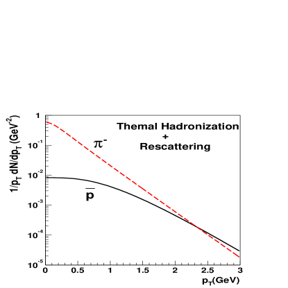
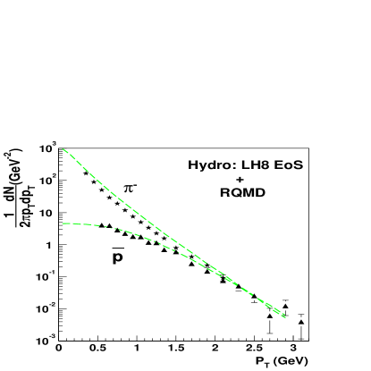
Figure 19: A comparison of $\pi^{-}$ and $\bar{p}$ spectra. (a) shows a simple thermal model with parameters discussed in the text. The spectra are relatively normalized. (b) shows an absolutely normalized comparison of the complete model spectra and PHENIX spectra PHENIX-Spectra .

IV.6 The Impact Parameter Dependence of Radial Flow

In peripheral collisions, hydrodynamic features should disappear since the mean free path becomes comparable to the root mean square radius $R_{rms}$. Because ideal hydrodynamics is scale invariant, the hydrodynamic stage of the model does not capture finite size effects which become increasingly important at larger impact parameters. However, this does not mean that the radial velocity is independent of impact parameter. The hydrodynamic lifetime scales approximately as $R_{rms}$; the flow velocity reflects this lifetime. Finite size effects make the total lifetime decrease more quickly than $R_{rms}$. Finite size effects are most important during the freezeout stage which is modeled with RQMD and therefore the hydro+cascade approach can capture some non-trivial features of the impact parameter dependence.

In the low $M_{T}$ region, pion-nucleon scattering in RQMD is largely responsible for the $\approx 500\,\mbox{MeV}$ anti-proton slope measured by the STAR collaboration STAR-Spectra . In the high $M_{T}$ region measured by the PHENIX collaboration PHENIX-Spectra , the hydrodynamic stage of the model is much more significant than hadronic rescattering. Fig. 20 shows the low and high $M_{T}$ slope parameters as a function of the number of participants in the collision. For each particle, the open symbols show the slope parameter without RQMD and the closed symbols show the slope parameter with RQMD. For both pions and kaons in the low and high $M_{T}$ regions, only a small impact parameter dependence is observed. The pion spectrum is cooled at all impact parameters.

Compare the nucleon and the $\phi$ slope parameters. In the low $M_{T}$ region, shown in Fig. 20(a), the nucleon slope exhibits a very rapid dependence on the number of participants. Approximately 40% of this slope is due to RQMD and the “Hydro Only” curve for the nucleon is relatively flat as a function of impact parameter. The nucleon and the $\phi$ have approximately the same mass but the $\phi$ is devoid of the strong $\Delta$ resonance which drives the flow in the nucleon system. Therefore, the “Hydro Only” curve for nucleons is similar to the “Hydro+RQMD” curve for the $\phi$.

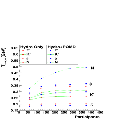
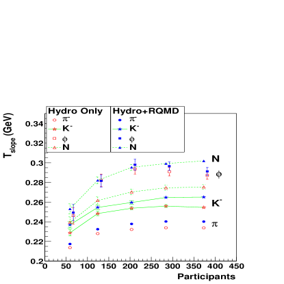
Figure 20: The (a) low $M_{T}$ and (b) high $M_{T}$ slope parameters (see Fig. 15) as a function of the number of participants in the collision.

Next, compare the nucleon and the $\phi$ slopes in the high $M_{T}$ region, shown in Fig. 20(b). Here $\pi N\rightarrow\Delta$ is less significant and RQMD is responsible for only $\approx 15\%$ of the nucleon slope. Consequently, RQMD makes up the small difference between the nucleon and the $\phi$ “Hydro Only” curves, and the final slope parameters of the two particles are similar in shape and magnitude. Experimentally, the difference in slope parameters between the nucleons and the $\phi$ can be used to assess the contribution of the hadronic phase in the low $M_{T}$ region.

Turning to the experimental data, we first examine the low $M_{T}$ region as measured by the STAR collaboration. We compare the model b-dependence of the anti-proton and $K^{-}$ slope parameters to the experimental data in Fig. 21 and  22. Comparing the anti-proton slopes for different EOS, we see that the rapid b-dependence is not a consequence of a change in EOS. Note that LH$\infty$ has a larger slope at small $M_{T}$ than LH8. This is an artifact of the exponential fit. The spectrum for LH$\infty$ in central collisions is shown in Fig 18 and is not exponential. The measured spectra are well described by an exponential in this region STAR-Spectra . Coarsely, the model reproduces the strong b-dependence of the anti-protons and the weaker b-dependence of the kaons. However, for more peripheral collisions, the measured slope parameters fall somewhat faster than the model predicts. Naively, this indicates that in the most peripheral collisions the hydrodynamic description is only beginning to work and finite size effects (e.g viscosity) should be taken into account in the QGP and mixed phases which are modeled with the hydrodynamics. The “Hydro Only” curves presented in Fig. 21 and 22 definitely do not reproduce the strong b-dependence of the slopes. With RQMD on the other hand, finite size effects during the late hadronic stages are modeled and most of the rapid b-dependence seen in the data is reproduced.

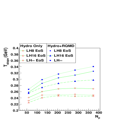
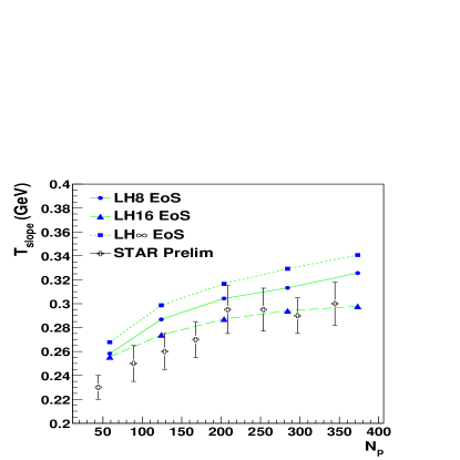
Figure 21: Model and preliminary STAR $K^{-}$ STAR-Spectra slope parameters in the fit range $0<M_{T}-M<0.5\,\mbox{GeV}$ as a function of the number of participants for different EOS. (a) compares model predictions for each EOS with and without the RQMD after-burner; (b) compares the model to data with the RQMD after-burner.

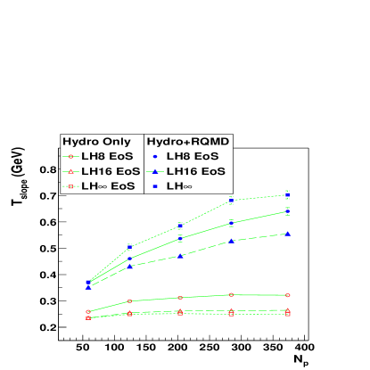
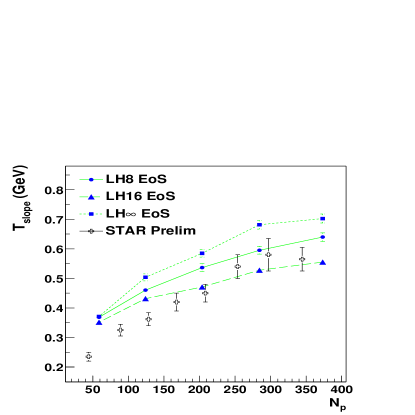
Figure 22: Model and preliminary STAR $\bar{p}$ STAR-Spectra slope parameters in the fit range $0<M_{T}-M<0.5\,\mbox{GeV}$ as a function of the number of participants for different EOS. (a) compares model predictions for each EOS with and without the RQMD after-burner; (b) compares the model to data with the RQMD after-burner.

Turning to the high $M_{T}$ region, the absolutely normalized model spectra are compared directly to the absolutely normalized PHENIX spectra for different centralities and particles in Fig. 23.

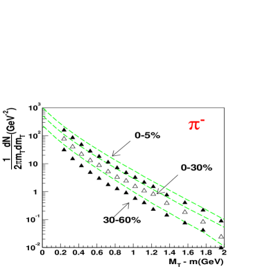
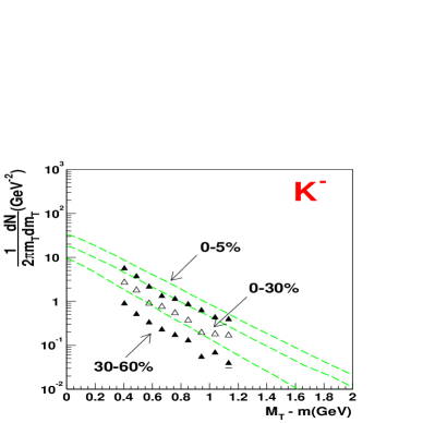
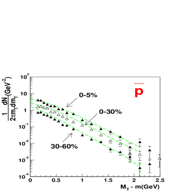
Figure 23: The absolutely normalized model spectra for LH8 compared to PHENIX spectra PHENIX-Spectra at different centralities. (a) is for $\pi^{-}$, (b) is for $K^{-}$ and, (c) is for $\bar{p}$.

For $K^{-}$ and $\bar{p}$ the spectrum is reproduced in the most central bin (0-5% central with $<N_{p}>=350$) and in the semi-peripheral bin (30-60% central with $<N_{p}>=76$). For pions, the spectral shape in the most central bin is reproduced. However, in the semi-peripheral bin, the pion spectrum resembles a power-law rather than a thermal spectrum. This change in shape from peripheral to central has been attributed to jet-quenching Wang-JetQuenching ; GDavid-JetQuenching .

V Elliptic Flow from the SPS to RHIC

In non-central collisions the particles emerge with an elliptic flow. The spectator matter flies down the beam pipe and the excited nuclear matter is formed in the transverse plane with an almond shaped distribution. Subsequently, if pressure develops in the system, the pressure gradients are larger in the impact parameter direction (the x-direction) than in the y-direction. Then, the excited matter expands preferentially in the x-direction. The magnitude of this elliptic response is quantified experimentally by expanding the distributions in a Fourier series

$$\frac{dN}{p_{T}\,dp_{T}\,dy\,d\phi} = \frac{dN}{2\pi\,p_{T}dp_{T}dy}(1+2\,v_{2}(p_{T},y)\,\cos(2\phi)$$ (27)

$$+...)$$

where $\phi$ is measured around the z-axis relative to the impact parameter, which points in the x direction. The $elliptic$ flow, $v_{2}(p_{T},y)\equiv\langle\cos(2\phi)\rangle_{p_{T},y}$, gives a measure of the dynamic response of the excited nuclear matter to the initial anisotropy.

The initial spatial anisotropy is quantified using the parameter $\epsilon$ (see Eq. 9). The hydrodynamic response is linear in $\epsilon$ Ollitrault-Elliptic and therefore $v_{2}$ is sometimes divided by $\epsilon$ to compare different impact parameters and nuclei Sorge-kink ; Voloshin-LowDensity . As the system expands, the eccentricity $\epsilon$ decreases. Since $\epsilon$ is the driving force behind the elliptic flow, the elliptic development finishes before the radial development. Therefore, elliptic flow is generated by the early pressure, although this statement must be qualified (see below). The spatial anisotropy that remains after the collision is quantified by $s_{2}$ (see Eq. 20). $s_{2}$ measures how much of the initial spatial anisotropy $\epsilon$ was not used during the collision for the production of elliptic flow.

V.1 Qualitative Changes from the SPS to RHIC

In Sect. IV.1 radial flow was used to constrain the EOS. The best (though certainly not unique) description of the data was given by LH8. For consistency, we require the same EOS to describe the elliptic flow data.

Fig. 24(a) shows integrated elliptic flow of pions

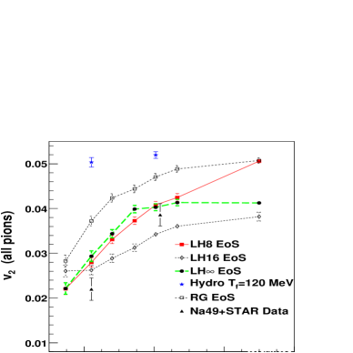
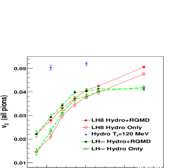
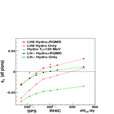
Figure 24: Panels (a)-(c) show three related quantities as a function of the total multiplicity in a PbPb collision at $\mbox{b}=6\,\mbox{fm}$. (a) shows the integrated elliptic flow $v_{2}$ of pions for different EOS and freezeout conditions; (b) shows the integrated elliptic flow $v_{2}$ with and without hadronic rescattering; (c) shows the spatial anisotropy $s_{2}$ with and without hadronic rescattering. At the SPS, the NA49 $v_{2}$ data point is extrapolated to b=6 fm using Fig. 3 in NA49-BDependence . At RHIC, the STAR $v_{2}$ data point is extrapolated to $N_{ch}/N_{ch}^{max}=0.545$ (b=6 fm in AuAu) using Fig. 3 in STAR-EllipticPRL .

as a function of the total multiplicity for different EOS. Fig. 24(b) shows the relative contribution of RQMD to the integrated elliptic flow. Note that elliptic flow increases for all EOS and dramatically so for LH8. Assume momentarily that elliptic flow for Hydro+RQMD stops developing at a temperature of $T\approx T_{c}\approx 165\,\mbox{MeV}$. (Note however that the radial flow develops well below this temperature). The dramatic increase of elliptic flow in Fig. 24(a) can be understood as the dynamic response of the QGP pressure. Recall Fig. 5(b), which plots anisotropy of the hydrodynamic stress tensor versus time and pay particular attention to the $T\approx T_{c}$ points (the solid symbols) on the LH8 and RG curves (ignore LH$\infty$ for now). At the SPS, the anisotropy of the stress tensor increases rapidly at first and then stalls. The final stress tensor anisotropy is small at the end of the mixed phase. At RHIC, elliptic flow develops more rapidly and stalls only when the anisotropy is large. Thus, provided the elliptic flow stops developing at $T_{c}$, the elliptic flow increases dramatically as the QGP pressure appears. For a RG EOS at the SPS, there is no mixed phase and no stall and consequently the RG elliptic flow is significantly larger than LH8 and the data. However with RHIC collision energies, LH8 begins to behave as an ideal QGP. Consequently, at RHIC the RG elliptic flow is only 20% larger than that of LH8 and of the data.

To understand when elliptic flow stops developing, it is important to track the spatial geometry of the underlying source. When the spatial anisotropy, $s_{2}$, is negative, the pressure drives elliptic flow. However, as $s_{2}$ approaches zero, the pressure gradients drive radial motion rather than elliptic motion. The elliptic development then stops. Fig. 24(c) shows the spatial anisotropy, $s_{2}$, for pions as a function of multiplicity from the SPS to RHIC. Compare the LH8 curves (the stars, the solid squares, and the open squares) seen in Fig. 24(c). The open squares (LH8 Hydro Only) show the spatial anisotropy, $s_{2}$, at the end of the mixed phase, the closed squares (LH8 Hydro+RQMD) show $s_{2}$ after the cascade, and the stars show $s_{2}$ when the hydrodynamic evolution is continued to $T_{f}=120\,\mbox{MeV}$. After the mixed phase (LH8 Hydro Only), the matter retains some of its initial almond shape. Continuing the hydrodynamics destroys the initial almond shape completely and increases $v_{2}$ by a factor of $\approx 2-3$ (see Fig. 24(c)). Cascading also changes the almond shape but increases $v_{2}$ by only a factor of $\approx 1.5$. In either case, $s_{2}$ crosses zero between the SPS and RHIC and therefore elliptic development in the hadronic stage ceases to be significant between the SPS and RHIC.

This fact is illustrated with Fig. 25 which contrasts the RQMD contribution to $v_{2}(p_{T})$ with the contribution of the hadronic phase in a pure hydrodynamic calculation at the SPS and RHIC.

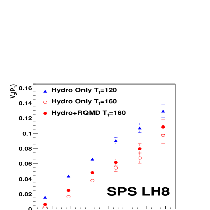
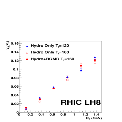
Figure 25: The dependence of $v_{2}(p_{T})$ on the switching temperature $T_{switch}$ at (a) the SPS and (b) RHIC for an impact parameter of $\mbox{b}=6\,\mbox{fm}$.

At the SPS, $v_{2}(p_{T})$ increases by a factor of two when the the hydrodynamics is continued to $T_{f}=120\,\mbox{MeV}$. When the hydrodynamics is replaced with RQMD, $v_{2}(p_{T})$ also develops but only by approximately $20\%$. At RHIC, the spatial asymmetry is completely destroyed by the end of the mixed phase and the elliptic development is frozen for all $p_{T}$. Continuing with the cascade or the hydrodynamics increases the elliptic flow marginally.

V.2 The Impact Parameter Dependence of Elliptic Flow

Fig. 26 shows the b or $N_{p}$ dependence of integrated pion elliptic flow at the SPS and RHIC.

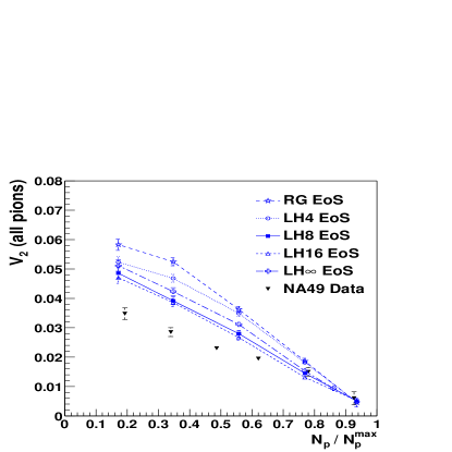
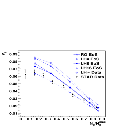
Figure 26: (a) $v_{2}$ for pions at the SPS as a function of participants (relative to the maximum) compared to NA49 data NA49-BDependence . (b) $v_{2}$ for charged particles at RHIC as a function of participants (relative to the maximum) compared to STAR data STAR-EllipticPRL .

The data restrict the underlying EOS. At the SPS, the data favor a soft EOS – LH $\geq$ $0.8\,\mbox{GeV/fm}^{3}$. LH4 and RG EOS generate too much elliptic flow. For LH8-LH16, the model is about $20\%$ above the data. However, the model to data comparison is not completely fair – the data points are integrated over rapidity, while the model points are only strictly valid for mid-rapidity. This probably accounts for the residual model/data discrepancy. As the latent heat is increased beyond LH32 to LH$\infty$ , the elliptic flow begins to rise. The origin of this elliptic flow was described in Htoh and results from the slow evaporation of particles in an asymmetrical fashion over a long time. This elliptic flow is generated without radial flow Kolb-NoFlow and the $p_{T}$ dependence of $v_{2}$ for nucleons (see below) is modified accordingly Kolb-NoFlow . At RHIC (Fig. 26(b)), the comparison is fair and the data again favor a relatively soft EOS, LH8-LH16. Thus the elliptic flow data at the SPS and RHIC are consistent with a single underlying EOS.

Note that the ordering of the EOS in Fig 26 differs at the SPS and RHIC. At the SPS, LH8 and LH16 generate approximately the same elliptic flow. At RHIC, the hard QGP phase lives for substantially longer with LH8 than with LH16 and therefore generates more elliptic flow. Additionally at RHIC, LH4 generates more elliptic flow than a RG EOS. Thus, the elliptic flow indicates that at high energy densities LH4 (with $c_{s}^{2}\approx 1/3$) has a larger speed of sound than a RG EOS (with $c_{s}^{2}\approx 1/5$). At asymptotically, high energy densities all EOS in the LH(x) family approach the massless ideal gas limit.

V.3 The $p_{T}$ Dependence of Elliptic Flow

Having discussed qualitative changes from the SPS to RHIC, we explore the $p_{T}$ dependence of elliptic flow. Experimental measurements are performed over a range of impact parameters. To find $v_{2}(p_{T})$ in a specific impact parameter range, $b_{min}<b<b_{max}$, the following integrals must be performed,

$$v_{2}(p_{T},y)_{b_{min}}^{b_{max}} \equiv \frac{\int_{b_{min}}^{b_{max}}v_{2}(p_{T},y;b)\,\frac{dN}{dy\,dp_{T}}(b)\,2\pi b\,db}{\int\frac{dN}{dy\,dp_{T}}(b)\,2\pi b\,db}.$$

Again, we drop the $y$, $b_{min}$ and $b_{max}$ labels below when it is not confusing. $v_{2}(p_{T})^{min-bias}$ denotes the elliptic flow integrated over all events, or $v_{2}(p_{T})_{0}^{\infty}$.

Fig. 27(a), (b) and (c) show $v_{2}(p_{T})^{min-bias}$

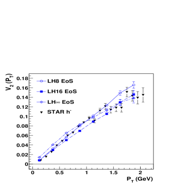
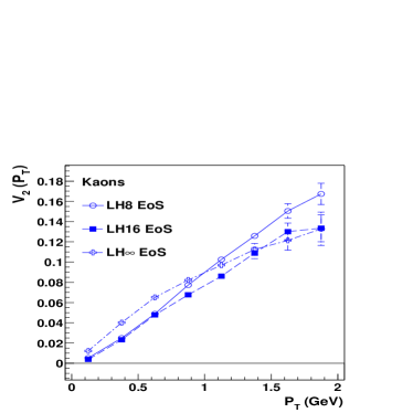
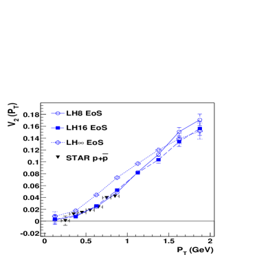
Figure 27: $v_{2}(p_{T})^{min-bias}$ (see Eq. V.3) for three different EOS compared to data. Panels (a), (b) and (c) are for negative hadrons, all kaons, and p+$\bar{\mbox{p}}$, respectively. The data are from STAR-EllipticPRL ; STAR-EllipticParticle .

for negative hadrons, kaons, and nucleons at RHIC. Look first at the negative hadrons (a): Although LH8 and LH16 both show a strong linear rise, the slope is smaller for LH16. For LH$\infty$, $v_{2}(p_{T})$ is curved and bends over. For small $p_{T}$, LH$\infty$ is above LH8, but by $p_{T}\approx 2.0\,\mbox{GeV}$, LH$\infty$ is substantially below LH8. The data show a strong linear rise and agree remarkably well with the slope of LH8. $v_{2}(p_{T})$ slightly favors LH8 over LH16. The kaon $v_{2}(p_{T})$ curve has the same shape and magnitude as the $h^{-}$ spectrum. At the SPS the kaon elliptic flow is slightly negative SPS-NegKaV2 . This anti-elliptic flow is most likely a remnant of the repulsive mean field observed at higher baryon densities. At RHIC, the baryon density is lower than at the SPS and kaons should flow along with the pions if the space time picture of the model is correct.

For nucleons, the $v_{2}$ spectral shape is different and is initially curved upwards. A useful thermal model has been given to explain the shape of $v_{2}(p_{T})$ Kolb-Radial ; SR-FlowProfile . For nucleons, LH8 and LH16 are concave up, indicating a strong radial expansion. By contrast, LH$\infty$ shows a linear rise in $v_{2}(p_{T})$, indicating a weak transverse expansion. As discussed in Sect. III, LH$\infty$ slowly evaporates particles into RQMD and generates elliptic flow only at small $p_{T}$. The curvature of $v_{2}(p_{T})$ for LH$\infty$ resembles the $p_{T}$ dependence expected if only surface evaporation were present Kolb-NoFlow . However, LH$\infty$ does develop a substantial radial flow over its long lifetime which gives the LH$\infty$ $v_{2}(p_{T})$ some shape. The data favor the strong transverse expansion of LH8 over the weak expansion of LH$\infty$.

We now demonstrate that pion nucleon scattering on top of a baseline elliptic flow is responsible for the curvature of $v_{2}(p_{T})$ seen in data. Fig. 28 shows $v_{2}(p_{T})$ with and without

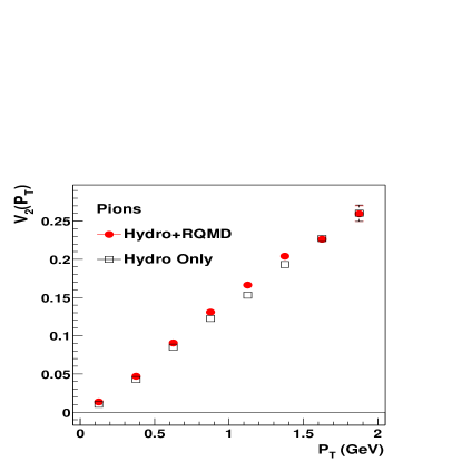
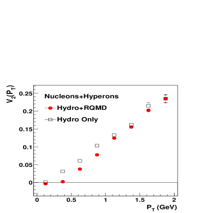
Figure 28: $v_{2}$ as a function of $p_{T}$ for (a) all pions and (b) nucleons+hyperons with and without the RQMD after-burner for AuAu collisions at b=6 fm, for LH8 EOS.

hadronic rescattering. Here the discussion parallels the discussion of the radial flow. Pion nucleon scattering increases the radial flow of the nucleon spectrum and cools the pion spectrum. Consequently the pion $v_{2}$ spectrum with the RQMD after-burner is slightly above the “Hydro Only” spectrum. Similarly, the nucleon $v_{2}$ spectrum with the after-burner is curved upward by $\pi-N$ scattering within RQMD. Similar features were found in all the EOS studied above.

Now to illustrate the impact parameter dependence, Fig. 29 shows the b-dependence of $v_{2}(p_{T})$.

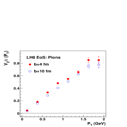
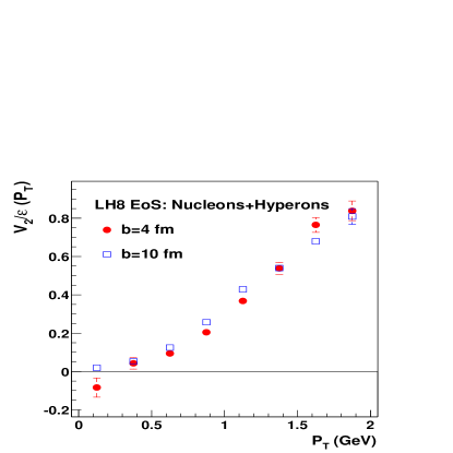
Figure 29: $v_{2}(p_{T})/\epsilon$ for semi-central (b=4 fm) and semi-peripheral (b=10 fm) collisions with LH8 EOS. Panel (a) is for pions and (b) is for nucleons+hyperons.

To compare different impact parameters, $v_{2}(p_{T})$ for pions and nucleons is divided by the initial space anisotropy $\epsilon$, for peripheral (b=10 fm) and semi-central (b=4 fm) collisions. The model response basically follows naive geometric considerations. However, closer inspection reveals that the model captures some finite size effects during the late hadronic stages. As the impact parameter is scanned, the total number of pions decreases roughly as the number of participants, and pion-nucleon scattering decreases similarly. Consequently, for central collisions pions show slightly larger elliptic flow at small $p_{T}$ while nucleons show a smaller (more curved) elliptic flow at small $p_{T}$. Thus, together these curves indicate a slightly stronger hadronic expansion in central collisions.

We now return to the SPS and compare the model to NA49 elliptic flow data. Fig. 30

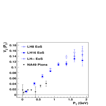
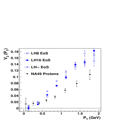
Figure 30: $v_{2}$ as a function of $p_{T}$ for pions and protons in PbPb collisions at the SPS. The data points are for events with $b\approx 6.5-8\,\mbox{fm}$ or more precisely for events with 45-60% of the beam energy in the NA49 zero-degree calorimeter NA49-EllipticPRL . The model points are the results of integrals between $\mbox{b}=6.5-8\,\mbox{fm}$ or $v_{2}(p_{T})_{6.5}^{8.0}$ as described by Eq. V.3. The model data comparison is not completely fair – the model points are for mid-rapidity while the data points have been integrated over rapidity (see text).

compares the model and data $v_{2}(p_{T})$ for pions and nucleons. These data are generally less well produced than at RHIC. Some caveats should be mentioned. The data are forward in rapidity, $4<y<5$, while strictly speaking, the model is only valid for mid-rapidity data (y=2.92). For pions, $v_{2}$ has a fairly flat rapidity dependence but the total abundance changes significantly from y=2.92 to y=5. For nucleons, $v_{2}$ has strong rapidity dependence and is almost a factor of two larger at mid-rapidity. At mid-rapidity, the elliptic flow is certainly stronger, which should improve the agreement with the model. Furthermore, in the forward rapidity region, the dynamics are complex; pions and nucleons have a significant directed flow indicating that details of stopping may play a significant role. In conclusion, much more data are needed to establish the applicability of hydrodynamics at the SPS.

V.4 Summary and Comparison

The principle motivation of this work was to demonstrate that the body of heavy ion data from the SPS to RHIC can be described with thermodynamics and hydrodynamics. To this end, we have compared of the hydro+cascade model of Htoh to the radial and elliptic flow data from the SPS and RHIC. A simultaneous analysis of available flow constrains the EOS. Only an EOS exhibiting the hard and soft features of the QCD phase transition systematically reproduces the observed radial and elliptic flow.

The model incorporates strong radial and elliptic flow, chemical freezeout at the phase boundary, subsequent hadronic rescattering and differential freezeout. With these ingredients, the model explains a number of features of the new RHIC data.

• The “anomalous” $\bar{p}/\pi^{-}$ ratio (which exceeds one for $p_{T}\sim 2\,\mbox{GeV}$) is a simple consequence of the increase in the radial flow and chemical freezeout. In a thermal picture, anti-protons are enhanced relative to proton-proton collisions. Then, the strong radial flow drives these anti-protons to large $p_{T}$. Subsequent hadronic rescattering makes the spectra cross.

• The $M_{T}$ spectra (which are “curved” as opposed to simply exponential) are readily explained in a hydro+cascade model. The curvature is due to a combination of the flow profile expected from hydrodynamics SR-FlowProfile ; SSH-FlowProfile and hadronic rescattering. With these ingredients, the mass dependence of the spectra measured by the STAR and PHENIX collaborations are naturally explained. The strong b-dependence of the STAR slope parameters for anti-protons STAR-Spectra is a consequence pion-nucleon scattering. In contrast, the slope parameter for the $\phi$, which suffers few hadronic collisions in the model, shows little b-dependence.

• The observed elliptic flow rises rapidly as a function of $p_{T}$ and favors a strong transverse expansion. Unlike the radial spectra, the elliptic spectra are less sensitive to hadronic rescattering and differential freezeout. Therefore, our results on the $p_{T}$ spectrum of $v_{2}$ are largely similar to the hydrodynamic analysis in Kolb-LowDensity ; Kolb-Radial .

These features are generic to a radially and elliptically expanding thermal source and do not immediately implicate hydrodynamics as the dynamic origin of the radial and elliptic flow. However, running hydrodynamic up to the phase boundary (with the same EOS) quantitatively reproduces the necessary radial and elliptic flow velocities both at the SPS and RHIC. In particular, hydrodynamics reproduces the observed changes from the SPS to RHIC:

• In a hydrodynamic framework, the radial flow velocity increases at high energy densities for an EOS with a phase transition to the QGP Ollitrault-MixedPhase ; Kataja-MixedPhase . At the SPS, LH8 gave the best agreement with spectra and predicted a $\approx 20\%$ increase in the radial flow velocity from the SPS to RHIC Htoh . The first RHIC spectra confirm the predictions of LH8 and the predictions of other hydrodynamic works Kolb-Radial ; Kolb-UU . Generally, LH8 has a smaller latent heat than that used in other works and therefore LH8 predicts a larger increase in the radial flow. In particular, already at RHIC, the $m_{T}$ spectrum of the $\Omega^{-}$ is significantly curved by the radial flow HydroUrqmd .

• At RHIC and to a lesser extent at the SPS, the magnitude of the integrated elliptic flow is reproduced. During the early stage of this work, a $\approx 40\%$ change in elliptic flow the SPS to RHIC was predicted and subsequently observed STAR-EllipticPRL . This increase is a direct consequence of the QGP pressure Kolb-UU ; Shuryak-QM99 and the early freezeout of elliptic flow at the SPS Htoh .

V.5 Fixing the EOS

Taking the radial and elliptic flow together, we argue that the momentum correlations in the data reflect the hydrodynamic response of excited matter exhibiting the soft and hard features of the QCD phase transition. For an EOS without softness, e.g. a resonance gas EOS, the flow of multi-strange baryons is dramatically missed (see Fig. 12). In addition, the elliptic flow is significantly too large both at the SPS and at RHIC (see Fig. 26(a) and (b)). These observations indicate that without softness the initial hydrodynamic response of the fireball is too strong.

For an EOS without a hard component, e.g. LH$\infty$, the spectra are significantly too soft both at the SPS and RHIC (see Fig. 11 and Fig. 18). The flow of the multi-strange baryons is even too small (see Fig. 12). Although LH$\infty$ generates a large $v_{2}$ by evaporating particles anisotropically through the freezeout surface, the $p_{T}$ dependence of this elliptic flow is qualitatively wrong (see Fig. 27). For LH$\infty$, hadronic rescattering does generate some transverse flow, but this transverse flow is insufficient to explain the strong $p_{T}$ dependence of the elliptic flow. The strong curvature for $v_{2}(p_{T})$ seen in the nucleon data implicates a violent explosion and this violent explosion is not generated by LH$\infty$. Out of all the EOS considered, the best agreement is found with LH8. The same EOS was deduced prior to the analysis of the first RHIC data Htoh . LH8 has a latent heat of $800~{}\mbox{MeV/fm}^{3}$ and represents a balance between soft and hard.

V.6 Outlook

Finally, we turn to open problems. Hanbury-Brown Twiss (HBT) correlations provide information about the spatial and temporal extent of the freezeout region. Such measurements have been performed at the AGS, the SPS Uli-Review and recently at RHIC STAR-Pion . Although the HBT radii fall with the pion pair momentum $K_{T}$ providing additional evidence for transverse flow Uli-Review , the measured radii at RHIC are approximately only 50% percent of our preliminary radii Teaney-HBT .

The dynamic origin of these small HBT radii is not understood and much more work is needed Hirano-HBT . The small radii indicate that although the final velocities are correctly reproduced within the model, the model expansion time is too long. Future experiments will measure HBT radii and deuteron production as a function of impact parameter and azimuthal angle. Such detailed experimental information is essential to a complete understanding of the excited matter produced in ultra-relativistic heavy ion reactions.

Acknowledgments The continued support of the nuclear chemistry group at Stony Brook is gratefully acknowledged. This work was supported in parts by the US-DOE grants DE-FG-88ER40388 and by DE-FG02-87ER 40331.

References

- (1) Quark Matter 1997, Nucl. Phys. A638, (1998).
- (2) Quark Matter 1999, Nucl. Phys. A661(1999).
-
(3)
Quark Matter 2001, to be published in Nucl. Phys. A,
Stony Brook, NY, January 15-20 (2001) ;
http://www.rhic.bnl.gov/qm2001/program.html - (4) E.V. Shuryak, Phys. Reports C61, 71 (1980).
- (5) e.g., M. Oevers, F. Karsch, E. Laermann, and P. Schmidt, Nucl. Phys. Proc. Suppl. 73, 465 (1999).
- (6) P. Braun-Munziger, J. Stachel, J.P. Wessels, N. Xu, Phys. Lett B344, 43 (1995).
- (7) F. Becattini, M. Gadzdzicki and J. Sollfrank, Eur. Phys. J. C5, 143 (1998)
- (8) J. Sollfrank, J. Phys. G23, 1903 (1997).
- (9) J. Cleymans and K. Redlich, Phys. Rev. C59, 354 (1999) ; J. Cleymans, H. Oeschler and K. Redlich, Phys. Rev.C59, 1663 (1999) ;
- (10) E.V. Shuryak and O.V. Zhirov, Phys. Lett. B89, 253 (1979).
- (11) e.g., R. Stock, in Quark Matter 1999, Nucl. Phys. A661, 419c (1999).
- (12) e.g., U. Heinz, Nucl. Phys. A685, 414 (2001) and references therein.
- (13) M. Gyulassy and X.N. Wang, Comp. Phys. Comm. 83, 307 (1994); Phys. Rev. D44, 3501 (1991).
- (14) D. Molnar and M. Gyulassy, nucl-th/0104073.
- (15) M. Bleicher and H. Stocker, hep-ph/0006147.
- (16) Josef Sollfrank et al, Phys. Rev C55, 392 (1997).
- (17) U. Ornik, M. Pluemer, B.R. Schlei, D. Strottman, R. M. Weiner Phys. Rev. C54 1381 (1996).
- (18) P.F. Kolb, J. Sollfrank, U. Heinz, Phys. Rev. C62, 054909 (2000).
- (19) P.F. Kolb, P.Huovinen, U. Heinz, H. Heiselberg, Phys. Lett B500, 232 (2001).
- (20) P. Huovinen, P.F. Kolb, U. Heinz, H. Heiselberg, Phys. Lett B503, 58 (2001).
- (21) D. Teaney, J. Lauret, and E.V. Shuryak, Phys. Rev. Lett. 86, 4783 (2001).
- (22) C.M. Hung, E.V. Shuryak, Phys. Rev. Lett. 75, 4003 (1995).
- (23) C. Greiner, D. H. Rischke, Phys. Rev. C54 1360 (1996).
- (24) NA49 Collaboration, T. Alber et al., Phys. Rev. Lett. 75, 3814 (1995).
- (25) PHOBOS Collaboration, B.B. Back et al, Phys. Rev. Lett. 85, 3100 (2000) ;
- (26) L. Van Hove, Z. Phys. C21, 93 (1983).
- (27) J. Blaizot and J.-Y. Ollitrault, Phys. Rev. D36, 916 (1987);
- (28) M. Kataja et al., Phys. Rev. D34, 794 and 2755 (1986).
- (29) J.-Y. Ollitrault, Phys. Rev. D46, 229 (1992)
- (30) D. H. Rischke et al.. Heavy Ion Physics 1, 309 (1995). nucl-th/9505014.
- (31) U. Heinz, Nucl. Phys. A661, 141c (1999).
- (32) S. Bass and A. Dumitru, Phys. Rev. C61, 064909 (2000).
- (33) M. Belacem et al., Phys. Rev. C58, 1727 (1998).
- (34) H. van Hecke, H. Sorge, N. Xu, Phys. Rev. Lett. 81, 5764 (1998).
- (35) P.F. Kolb, J. Sollfrank, U. Heinz, Phys. Lett. B459, 667 (1999).
- (36) H. Sorge, Phys. Rev. C 52, 3291 (1995).
- (37) J.D. Bjorken, Phys. Rev. D27, 140 (1983).
- (38) D. Teaney, in preparation.
- (39) F. Cooper and G. Frye, Phys. Rev. D10, 186 (1974).
- (40) L.D. Landau and E.M. Lifschitz, Fluid Mechanics, 2nd Edition (Butterworth and Heinemann,1987)
- (41) M. Gyulassy and T. Matsui, Phys. Rev. D29, 419 (1984).
- (42) R.J. LeVeque, Numerical Methods for Conservation Laws, (Birkhäuser-Verlag,1990).
- (43) V. Schneider et al., J. Comput. Phys. 105, 92 (1993).
- (44) Dirk H. Rischke, Yaris Pusun, Joachim A. Maruhn, Nucl. Phys. A595, 346 (1995) ; Nucl. Phys. A595, 383 (1995).
- (45) P.F. Kolb, U. Heinz, P. Huovinen, K.J. Eskola, K. Tuominen, hep-ph/0103234.
- (46) P. Jacobs and G.Cooper, STAR SN402(1999).
- (47) STAR Collaboration, C. Adler et al., Phys. Rev. Lett 86, 4778 (2001).
-
(48)
PHOBOS Collaboration, B.B. Back et al, submitted to Phys. Rev.
Lett.,
http://www.phobos.bnl.gov/Publications/Ph_pub.htm - (49) PHENIX Collaboration, K. Adcox et al., Phys. Rev. Lett. 86, 3500 (2001).
- (50) PHOBOS Collaboration, B.B. Back et al, submitted to Phys. Rev. Lett. nucl-ex/0105011.
- (51) S. Soff, S.A. Bass, and A. Dumitru, Phys. Rev. Lett 86, 3981 (2001).
- (52) R. Venugopalan and M. Prakash, Nucl. Phys. A546, 718 (1992).
- (53) J.P. Blaizot and J.-Y. Ollitrault, Nucl. Phys. A458, 745 (1986).
- (54) S.M. Johns, P.J. Ellis, J.M. Lattimer, Astrophys. J. 473, 1020 (1996).
- (55) F. Cooper, G. Frye, E. Schonberg, Phys. Rev. D11, 192 (1975).
- (56) Cs. Anderlik et al., Phys. Rev. C59, 388 (1999) and references therein.
- (57) K.A. Bugaev, Nucl. Phys. A606, 559 (1996).
- (58) D. Teaney, Ph.D. Thesis, State University of New York at Stony Brook (2001).
- (59) E. Schnederman, J. Sollfrank, U.Heinz, Phys. Rev. C48, 2462 (1993).
- (60) H. Sorge, Phys. Rev. Lett. 78, 2309 (1997).
- (61) H. Sorge, Phys. Lett. B402, 251 (1997).
- (62) H. Sorge, Phys. Rev. Lett 82, 2048 (1999).
- (63) H. Sorge, Phys. Rev. Lett. 82, 2048 (1999).
- (64) STAR Collaboration, C. Adler et al. , nucl-ex/0107003. Submitted to Phys. Rev. Lett.
- (65) C.M. Hung, and E. Shuryak, Phys. Rev. C57, 1891 (1998).
- (66) NA49 Collaboration, H. Appelshäuser et al., Phys. Rev. Lett. 82, 2471 (1999).
- (67) D. H. Rischke and M. Gyulassy, Nucl. Phys. A608, 479 (1996).
- (68) E. Andersen et al., WA97 collaboration, Phys. Lett. B433, 209 (1998); R. Lietava for the WA97 collaboration in Proc. Strangeness 98, J. Phys. G: Nucl. Part. Phys. 25, (1999).
- (69) G. Roland for the NA49 Collaboration, Nucl. Phys. A638, 91c (1999).
- (70) P.J. Siemens and J.O. Rasmussen, Phys. Rev. Lett. 42, 880 (1979).
-
(71)
M. Caldéron, for the STAR Collaboration, at Quark Matter 2001 QM2001 ;
STAR Collaboration, C. Adler et al, to be submitted
to Phys. Rev. Lett.
http://www.star.bnl.gov/ . - (72) J. Velkovska, for the PHENIX Collaboration, at Quark Matter 2001 QM2001 ; nucl-ex/0105012.
- (73) I. Vitev and M. Gyulassy, nucl-th/0104066.
- (74) X. Wang, at Quark Matter 2001 QM2001 .
- (75) G. David, for the PHENIX Collaboration, at Quark Matter 2001 QM2001
- (76) S.A. Voloshin and A.M. Poskanzer, Phys. Lett. B474, 27 (2000).
- (77) A.M. Poskanzer and S.A. Voloshin for the NA49 Collaboration, Nucl. Phys. A661, 341c (1999).
- (78) STAR Collaboration, K.H. Ackermann et al., Phys. Rev. Lett 86, 402 (2001).
- (79) P. Huovinen, P.F. Kolb, U. Heinz, in Quark Matter 2001; nucl-th/0104020
- (80) Shunji Nishimura for the WA98 Collaboration, Nucl. Phys. A661, 464c (1999).
- (81) NA49 Collaboration, H. Appelshäuser et al., Phys. Rev. Lett. 80, 4136 (1998).
- (82) E.V. Shuryak in QM ’99 , Nucl. Phys. A661, 119c (1999);
- (83) e.g., U. Heinz and B.V. Jacak, Ann. Rev. Nucl. Part. Sci, 49, (1999).
- (84) STAR Collaboration, C. Adler et al., Phys. Rev. Lett. 87, 082301 (2001).
-
(85)
D. Teaney, RHIC-INT Workshop 2001. Lawrence Berkley National Laboratory, May 2001.
http://www-rnc.lbl.gov/ nxu/workshop/rww01.html - (86) e.g., Tetsufumi Hirano et al., nucl-th/0110009.