THE NUCLEAR PIONS AND QUARK DISTRIBUTIONS
IN DEEP INELASTIC SCATTERING ON NUCLEI

Abstract

We propose simple Monte Carlo method for calculating parton distribution in nuclei. Only events satisfying the exact kinematical constrains of the corresponding deep-inelastic reaction probing given nuclear distribution are selected to form the final distribution we are looking for. The EMC effect is automatically included by means of two parameters, which characterize the change of the nuclear pion field. Good agreement with experimental data in the broad range of variable $x$ is obtained.

12.38Aw; 12.38.Lg; 12.39.-x

1 Introduction

The study of partonic distributions inside the nucleon and nuclei has already long history [1]. Here we shall describe simple Monte Carlo method for calculating parton distributions in nuclei with special emphasis on the observed differences between such distributions for free and nuclear nucleons (known under the name EMC-effect) [2]. The parton picture of nucleon was originally formulated in the infinite momentum frame [3]. However, nuclear effects are more visible in the nucleon (or nuclear) target rest frame. Such change of frames has profound dynamical consequences. Whereas in the infinite momentum frame partons can be treated as on-shell objects (with some small current masses), in the rest frame they are dressed, far off-shell objects with masses consisting substantial part of the nucleon mass. The important point is how to find in this frame the proper parton energy. The nucleon is no longer contracted by Lorentz transformation and the corresponding interaction picture is complicated one. The nuclear parton density distributions are therefore obtained by generating initial parton momenta in nucleons and calculating the corresponding light-cone longitudinal momentum fractions, the so called Bjorken $x=x_{B}$, which must be identical in both frames.

Our approach is based on the model where valence parton momenta in hadron at rest are calculated from a spherically symmetric Gaussian distribution with a width derived from the Heisenberg uncertainty relation, whereas the sea parton contributions result from similar gaussian distribution but with a width dictated by the presence of virtual pions in hadron [2]. When going to the nuclear case these initial gaussian momentum distributions are changed accordingly in order to account for the presence of nuclear medium (like rescattering effects or changes in the virtual pion clouds in the nuclear matter). The energy momentum conservation is always strictly imposed and plays vital role in getting our results. The nuclear parton density distributions are then obtained by generating initial parton momenta of nucleons and calculating the corresponding light-cone longitudinal momentum fractions $x_{B}$.

2 Deep Inelastic Scattering

We start with short recollection of necessary theoretical points. In the deep inelastic electron-nucleon scattering the cross section is given by:

$$d\sigma=L_{\mu\nu}W^{\mu\nu}$$ (1)

where the hadronic tensor $W^{\mu\nu}$ can be expressed in terms of electromagnetic currents as:

$$W_{\mu\nu}=\int d^{4}p\exp(iq\xi)<p\mid J_{\mu}J_{\nu}(0)\mid p>.$$ (2)

The spatial variable $\xi$ is directly connected to the correlation length existing in this process. The virtual foton momentum transfer is given by:

$$q=(\nu,0,0,-\sqrt{\nu^{2}+Q^{2}}).$$ (3)

In the Bjorken limit $Q^{2}\rightarrow\infty$ the $x=Q^{2}/2M\nu\approx j^{+}/p^{+}$ is fixed and $q^{2}/\nu^{2}\rightarrow 0$. In this limit $q^{-}=q^{0}-q^{3}\rightarrow\infty$ but $q^{+}=-Mx/\sqrt{2}$ remains finite. These imply $\xi^{+}\rightarrow 0$ and $\xi^{-}\unlhd\sqrt{2}/Mx$. Alltogether this gives the following restrictions for $\xi$:

$$\xi_{0}\leq 1/Mx,\qquad\xi_{z}\equiv z\leq 1/Mx.$$ (4)

We have therefore two resolutions scales in deep inelastic scattering:

• $1/\sqrt{Q^{2}}$ connected with virtuality of $\gamma$ probe. Any two different $Q^{2}$ resolutions are connected via well known A-P evolution equation [4].

• $\frac{1}{Mx}=z$ being distance how far can propagate the anti-quark in the medium, see Fig.1. Notice that small $x$ means a relatively large correlation length $z$. Because final state quark interaction within the nuclear envirovment is practically not known the small $x$ region opens room for different phenomenological models and in this paper we shall propose a new mechanism for the nuclear shadowing.

Deep inelastic scattering of electrons on nuclear targets can be regarded as two step process: at first nucleus is replaced by composition of nucleons and (effective) pions representing quanta of nuclear binding forces, then impinging electrons interact with partons (quarks) composing those nucleons and pions. Formally it means that nuclear partonic distribution (structure function) $F_{2}^{A}$ can be written as convolution,

$$F^{A}_{2}(x_{A})/x_{A}=A\int\int dy_{A}dx\delta(x_{A}-y_{A}x)\rho^{A}(y_{A})F^{N}_{2}(x)/x,$$ (5)

of nucleon distribution function in the nucleus, $\rho^{A}(y_{A})$, and structure function of free nucleon, $F^{N}_{2}(x)$. The $x_{A}/A$ is the ratio of quark and the nucleus longitudinal momenta (i.e., it is the Bjorken variable for the nucleus) whereas $y_{A}/A=p^{+}/P^{+}_{A}$ is the ratio of the nucleon and nuclear longitudinal momenta. Finally $x$ is the ratio of the quark and nucleon longitudinal momenta (the Bjorken variable for the nucleon, $x=x_{B}$).

In the on-shell relativistic approach the nucleon distribution function is connected to the well known nucleon spectral function $S_{N}$ (discussed in the next section):

$$\rho^{A}(y_{A})=\int d^{4}p\delta\left(y_{A}/A-p^{+}/P^{+}\right)S_{N}(p^{o},{\bf p}).$$ (6)

In the mean field approximation $S_{N}(p^{o},{\bf p})=n(p)\delta(p_{o}-(m+e(p))$, where $e(p)$ is the nucleon single particle energy. This expression should be corrected by the incident flux factor (see eq.(8). It turns out, however, that even then one cannot describe the EMC data without inclusion of higher order nucleon-nucleon correlations (with additional free parameters and all uncertainties of off shell behavior of nucleons it brings in) [5].

3 Nuclear Relativistic Mean Field.

In the nuclear relativistic mean field (RMF) method electrons collide with nucleons which are moving in some constant average scalar and vector potentials in the rest frame of the nucleus according to the equation:

$$[{\hbox{$\boldmath{\alpha}$}}\cdot{\bf p}+\beta(m+U_{S})-(e_{N}-U_{V})]\psi=0.$$ (7)

Here $U_{S}=-g^{2}_{s}/m^{2}_{s}\rho_{s},~{}U_{V}=V_{\mu}\delta_{\mu 0}=g^{2}_{v}/m^{2}_{v}\rho$ with $g_{i},\ m_{i}\ (i=s,v)$ being the scalar or vector meson coupling constants and their masses, respectively, whereas $\rho_{s}=\sum_{i}\psi^{+}_{i}\beta\psi_{i}$ and $\rho=\sum_{i}\psi^{+}_{i}\psi_{i}$ are the scalar and the fourth component vector densities, respectively. The scalar and vector mean fields were investigated successfully in nuclear Dirac phenomenology with the values $U_{V}=300,U_{S}=-400$ [MeV$(\rho/\rho_{0})]$ $\rho_{0}=0.17fm^{-3}$ [6]. It turns out that $U_{S}$ and $U_{V}$ usually cancel each other in the energy or external response functions but their relatively big values can explain the enhancement of the spin-orbit part of nucleon-nucleus optical potential . It was shown [8] that $\rho^{A}(y_{A})$ depends on both the scalar and vector nuclear fields:

$$\rho^{A}(y_{A})={4\over\rho}\int{d^{4}p\over(2\pi)^{4}}S_{N}(p^{o},{\bf p})(1+p^{*}_{3}/E^{{}^{*}}(p))\delta(y-(p_{o}+p^{*}_{3})/\mu),$$ (8)

where $\mu$ is equal to the nucleon chemical potential, factor $(1+p^{*}_{3}/E^{{}^{*}}(p))$ corrects (6) for relativistic effects and the nucleon spectral function is taken in the RMF approach to be equal $S_{N}=n(p)\delta(p^{o}-(E^{{}^{*}}(p)+U_{V}))$. Eq. (8) can be simplified and written as:

$$\rho^{A}(y_{A})={3\over 4}(v^{2}_{A}-(y_{A}-1)^{2})/v^{3}_{A},$$ (9)

where $v_{F}=(\mu/m)(p_{F}/E_{F}^{{}^{*}})$, $v_{A}=p_{F}/E^{{}^{*}}_{F}$ and $y$ is restricted to region $0<(E_{F}^{{}^{*}}-p_{F})<my<(E_{F}^{{}^{*}}+p_{F})$. It means that all nuclear dependence is hidden in the nucleon chemical potential, which is, however, too weak (about $8$ MeV smaller than $m$) to reproduce the minimu seen in the EMC data [9] at $x=0.7$ (cf. curve $(a)$ in Fig. 2).

4 Proposed model for parton distribution in nuclei

Let $j$ denote four-momenta of struck parton (probed by current with virtuality $Q^{2}_{0}$) selected (for valence quarks) from Gaussian primordial distribution with width $0.172$ GeV, and $r$ the respective four-momentum of hadronic remnants. Let also $W$ and $W^{\prime}$ denote their respective invariant masses. Events are accepted if:

$$0\leq j^{2}\leq W^{2},0\leq r^{2}\leq W^{\prime 2}$$ (10)

The sea parton distribution is given by the convolution of the pionic component of the nucleon, $f_{\pi}(x;Q^{2}_{0})$, and the parton structure of pion, $f_{pion}(x;Q^{2}_{0})$, obtained from the same Gaussian primodial distribution as used for valence partons,

$$f_{s}(x;Q^{2}_{0})=\int\frac{dy}{y}f_{\pi}(y,Q^{2}_{0})f_{pion}(x/y;Q^{2}_{0}).$$ (11)

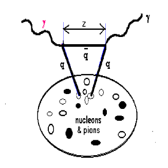
Figure 1:

Figure 2:

The characteristic behaviour of the sea partons is derived from the pion distribution in the nucleon, which was again parametrized by Gaussian distribution, this time with a smaller width equal to $0.052$ GeV. The overall partonic distribution is therefore given by ($Q_{0}^{2}=1$ GeV²)

$$F_{2}(x;Q^{2}_{0})=f_{v}(x,Q^{2}_{0})+f_{s}(x;Q^{2}_{0}).$$ (12)

Our results for R(x)=$F_{2}^{Fe}$/$F_{2}^{D}$ are presented with Monte Carlo error as (b) in Fig.2. For small $x$ the crucial factor turns out to be the change of nuclear virtual pion cloud connected with exchanged mesons responsible for the the nuclear forces [2]. In order to be able to fit data in this region we have to adjust in our model the value of the parameter which determines the relative number of the (effective) intermediate pions (assumed to mediate nucleon-nucleon interaction). In our model only part of pions contribute to the sea quark structure function of the nucleon whereas the other part is responsible for the the nucleon-nucleon interaction. Because for small $x$ the scale $z$ shown in Fig. 1 becomes comparable or bigger then the nucleon size, the expected range of nuclear forces also grows accordingly. Therefore for small values of $x$ the part of pionic contribution can ”disappear” during the interaction with the electromagnetic probe and consequently gives no contribution to the nuclear structure function. In our case up to $12\%$ of pions are excluded from interaction by this mechanism.

For intermediate $x$ ($\sim 0.7$) the minimum in the EMC ratio is obtain by adjusting the nucleon size in the medium (strictly speaking the size of the valence parton momentum distribution). The corresponding increase of this width from 0.18GeV to .172GeV produces both the minimum for $\sim 0.7$ and the maximum for $x$ around $0.1$. In hadronic language this change corresponds to some spreading of the pionic cloud outside the nucleon.

5 Summary

We obtain very good fit to the data on deep inelastic scatterings with ${}^{56}Fe$ using only two physically motivated parameters. The first describes decrease of width of the primordial gaussian valence quark distributions (it points towards the possible deconfinement of quarks in nuclear matter and to chiral symmetry restoration). The second parameter diminish the amount of nuclear pions below $x=0.1$ due to the shadowing effect.

References

- [1] Cf., for example, D.F. Geesaman, K. Saito and A. W. Thomas, Ann. Rev. Nucl. Part. Sci. 45, (1996) 137, and references therein.
- [2] J.Rożynek and G.Wilk, Phys. Lett. 473 (2000) 167.
- [3] J. D. Bjorken and E. A. Paschos, Phys. Rev. bf 185 (1969) 1975.
- [4] G. Altareli and A. Parisi, Nucl. Phys. B126 (1977) 298.
- [5] O. Benhar, V.R. Panderipande and I. Sick, Phys. Lett. B489, (2000) 131.
- [6] L. Celenza and C. Shakin, Relativistic Nuclear Physics, (World Scienfic, 1986).
- [7] B. D. Serot and J. D. Walecka, Adv. Nucl. Phys. 16 (1986).
- [8] M. Birse, Phys. Lett. B299, (1993) 188, J. Rożynek, Int. Journal Mod. Phys. E9 (2000) 195.
- [9] M. Arneodo et al., Nucl. Phys. B481 (1997) 3; S. Dasu at al., Phys. Rev. Lett. 64 (1988) 2591.
- [10] J. Zabolitsky and G. Ey, Phys. Lett. 76B (1983) 234.