QUADRUPOLE OSCILLATIONS AS PARADIGM OF THE CHAOTIC MOTION IN NUCLEI.(Part 1)

We have presented a complete description of classical dynamics generated by the Hamiltonian of quadrupole nuclear oscillations and identified those peculiarities of quantum dynamics that can be interpreted as quantum manifestations of classical stochasticity. Particular attention has been given to investigation of classical dynamics in the potential energy surface with a few local minima. A new technique is suggested for determination of the critical energy of the transition to chaos. It is simpler than criteria of transition to chaos connected with one or another version of overlap resonances criterion. We have numerically demonstrated that for potential with a localized unstable region motion becomes regular at the high energy again, i.e. transition regularity-chaos-regularity $\left({R-C-R}\right)$ takes place for these potentials. The variations of statistical properties of energy spectrum in the process of $R-C-R$ transition have been studied in detail. We proved that the type of the classical motion is correlated with the structure of the eigenfunctions of highly excited states in the $R-C-R$ transition. Shell structure destruction induced by the increase of nonintegrable perturbation was analyzed.

PACS numbers: 05.45.+b, 24.60.La, 21.10.-k, 03.65. Sq.

1 Introduction

1.1 Formulation of the problem

Quite often in the different divisions of physics statistical properties are introduced by means of postulates or hypotheses that are self-justified within some limiting case. Such an approach suggests an existence of a priori mechanism of randomness the nature of which lies usually outside the theory under discussion. For systems with a small number of degrees of freedom the results obtained in the thermodynamic limit look at least questionable. At the moment, however, one can consider as rigorously established fact an existence of such dynamical systems with a small number of degrees of freedom for which under certain conditions classical motion is distinguishable from random no matter what the definition of this notion we are using [1, 2, 3, 4, 5, 6]. Typical features of these systems are nonlinearity and absence of both external source of randomness and dissipation the mechanism of which is equivalent to the existence of random forces on a molecular level. Thus, using such synonyms for the term ”random” as ”chaotic”, ”stochastic”, ”irregular” one can state that there exist such systems with a finite number of degrees of freedom, for which these notions express adequately internal fundamental properties that comprise an important and interesting subject for investigation. For the last 30-40 years has been taken place a rather difficult recognition of the fact that chaotic motion is as usual in systems with more than one degree of freedom as regular motion. Instances of a chaotic motion have been found practically in every field of physics, and their number permanently continues to grow [1, 2, 3, 4, 5, 6].

Recent progress in understanding of the chaotic aspects of nonlinear dynamical systems is causing a rebirth of interest in the nuclear dynamics. Indeed, because of the richness of experimental data and sufficiently precision of the theory, the nuclear dynamics provides a very useful realistic model for studying classical dynamical chaos and quantum manifestations of the classical stochasticity.

Conception of chaos has been introduced in the nuclear theory within the last fifteen years [7, 8, 9, 10, 11, 12, 13, 14, 15, 16, 17, 18, 19, 20]. This conception brought birth to the new notion in the nuclear structure [7, 10, 11, 13, 21], nuclear reactions [8, 14, 20], could resolve a sequence of the very old contradictions in the nuclear theory [13, 22]. A radically new universal approach to the problem of statistical properties of the energy spectra was developed on the basis of the general nonlinear theory of dynamical systems [23]. Considerable advances have been made in the area of concrete nuclear effects: single particle in a deformed potential [11], nuclear fission [9], Ericson’s fluctuations [24], dynamics of the $3\alpha$ - linear chain [25], transition order-chaos-order in the roto-vibrational nuclear model [53, 54] etc. Finally, straightforward observations of the chaotic regimes in the course of mathematical simulations of the heavy-ions reactions [8] are evidence in favour the general considerations.

According to Baranger [13] there are two possible philosophies in nuclear physics.

Philosophy I. Nuclei are complicated, and chaos comes out of this complication. We expect to find chaos almost everywhere in nuclear physics. The interesting information is contained in those few places in which chaos is absent. We must look for non-chaos.

Philosophy II. Chaos is a property of simple systems; otherwise it’s no fun at all. The interesting new information is to be found in those simple areas of nuclear physics which we used to think we could understand, but which turn out to be chaotic. We must look for chaos.

The basis of present report is the philosophy of simple chaos - Philosophy II. Within the limits of this philosophy a general investigation of any nonlinear dynamical system involves the following steps.

1. An investigation of classical phase space with the aim of detection of chaotic regimes; numerical investigation of the classical equations of motion .

2. Analytical estimation of the critical energy for the onset of global stochasticity.

3. Test for quantum manifestations of classical stochasticity (QMCS) in the energy spectra, eigenfunctions and wave packet dynamics.

4. A consideration of the interrelationship between stochastic dynamics and concrete physical effects.

The basic subject matter of proposing report is to realize the outlined program, at least partially, for the large-amplitude quadrupole oscillations of nuclei (QON). We shall organize this paper as follows.

In the first part (section 2.1-2.7) we present complete description of classical dynamics generated by the Hamiltonian of quadrupole oscillations. This description contains

1. The scale analysis of the Hamiltonian (QON).

2. The discussion of the topological peculiarities of deformation potential.

3. The analytical estimations of critical energy of the transition to chaos.

4. The construction of the approximate integrals of motion with the help of normal forms.

5. The analysis of dynamics in the region of parameters space where the deformation potential has some local minima; the introduction of the concept of mixed state.

6. The general conception of reconstruction of regular motion at high energies for the systems with localized region of instability; the transition regularity-chaos-regularity as a particular realization of this conception.

7. Demonstration of the chaotic regimes in heavy-ions reactions.

In the second part peculiarities of quantum dynamics of considered system, which can be interpret as the QMCS. For this purpose in this part of the report were discussed

1. The Birkhoff’s-Gustavson’s quantum normal forms.

2. The change of statistical properties of the energy spectra in $R-C-R$ transition.

3. The change of the structure of wave functions in $R-C-R$ transition.

4. The destruction and the reconstruction of the shell structure in $R-C-R$ transition.

5. The dynamics of wave packets.

Thus, the distinctive feature of the suggested report is that all complex of questions connected with the investigation both classical stochasticity and QMCS is considered in the context of the unique dynamical system.

As for circle of readers whom this report is counted on, then on the one hand we would like to pay attention of experts in all areas of chaos to perspective field of application of general theory of nonlinear dynamical systems, and on the other hand to persuade nuclear experts that ideology of simple chaos can be equally useful just as traditional statistical approaches.

For convenience of the latter a brief summary of definitions and concepts used in description of stochastic motion in Hamiltonian systems will be given in section 1.2.

1.2 Classical stochasticity: some definitions

The classical dynamics of Hamiltonian systems with N degrees of freedom is described by the canonical equations of motion

$$\dot{p}_{i}=-\frac{{\partial H}}{{\partial q_{i}}},\quad\dot{q}_{i}=\frac{{\partial H}}{{\partial p_{i}}}\quad\left({1\leqslant i\leqslant N}\right)$$ (1)

where $H\left({\vec{p},\vec{q}}\right)$ is the Hamiltonian of system. The function of dynamical variables $F\left({\vec{p},\vec{q}}\right)$ is such that

$$\left\{{F,H}\right\}=0$$ (2)

where $\left\{{.,.}\right\}$ are Poisson’s brackets and it is called the integral of motion. If there are $N$ independent integrals $F_{i}\left({1\leqslant i\leqslant N}\right)$, such that $\left\{{F_{i},F_{j}}\right\}=0$, then the system (1) is integrable.

For integrable system one can introduce such canonical variables action-angle $\left({I_{i},\theta_{i}}\right)$ that Hamiltonian will be the function of only variables of action

$$H\left({\vec{p},\vec{q}}\right)=H\left(I\right)$$ (3)

The region labeled by fixed $I$ , to which the motion is confined, is therefore an $N$ -dimensional torus in the $2N$ -dimensional phase space. Any phase point that lies on a given torus at any time remains on it for all future times, so the torus itself is invariant under the Hamiltonian flow, and is known as an invariant torus. The motion on an invariant torus is given by

$$\theta_{i}\left(t\right)=\omega_{i}t+\theta_{i}\left(0\right)$$ (4)

where angular frequency vector $\omega_{j}$ can be written as

$$\omega_{i}=\frac{{\partial H}}{{\partial I_{i}}}$$ (5)

In this case the motion is a quasiperiodic function of time with at least $m$ independent frequencies. If the $\omega_{k}$ are not rationally related, that is, there are no integers $s_{i}$ , such that

$$\sum\limits_{i}{s_{i}\omega_{i}=0\left({s\neq 0}\right)}$$ (6)

then the phase point passes arbitrary close to every point of the torus and it is not difficult to show that the time average of function is equal to the average of the function over the angle variables. Thus the motion on the torus is ergodic. If (6) is satisfied for some nonzero integer vector s, than is a resonance, and $N$ -tori are made up of tori of lower dimension, to which the motion is confined. Such $N$ -tori are degenerated. The particular case of integrable system is the system with separable variables.

In the general case the system with two or more degrees of freedom is not integrable and can perform both quasiperiodic (regular) and stochastic motion. The distinctive feature of stochastic motion is instability, exhibiting in exponential divergence of close trajectories. If $x(t)$ and $x^{\prime}(t)$ are two trajectories close at $t=0$ in phase space, then during stochastic motion

$$\Delta\left(t\right)=\left|{x\left(t\right)-x^{\prime}\left(t\right)}\right|\approx\Delta\left(0\right)e^{\sigma_{i}\left(t\right)}$$ (7)

at sufficiently small $\Delta\left(0\right)$. Quantity $\sigma_{i}$ is called the maximal Liapunov exponent and is determined as

$$\sigma_{i}\left(x\right)=\lim_{t\rightarrow\infty,\Delta(0)\rightarrow 0}\left({\frac{1}{t}\ln\frac{{\Delta\left(t\right)}}{{\Delta\left(0\right)}}}\right)\left({x=x\left(0\right)}\right)$$ (8)

The system with $D$ -dimensional phase space is characterized by the set of $\Delta$ Lyapunov exponents $\sigma_{i}$ , which are numbered in order of decreasing. The points belonging to trajectory possess equal values $\sigma_{i}\left(x\right)$ . The motion is called stochastic if for trajectory $\sigma_{i}>0$ and regular if $\sigma_{i}=0$ .

Kolmogorov’s entropy $h$ is connected with Lyapunov exponents. For given stochastic trajectory

$$h=\sum\limits_{\sigma_{i}>0}{\sigma_{i}}$$ (9)

At stochastic motion the correlation function

$$B\left({f,g,\tau}\right)=\left\langle{f\left({t+\tau}\right)g\left(t\right)}\right\rangle-\left\langle{f\left(t\right)}\right\rangle\left\langle{g\left(t\right)}\right\rangle$$ (10)

(corner brackets $\left\langle{...}\right\rangle$ denote the averaging on time, and $f\left(t\right)=f\left({\vec{p},\vec{q}}\right)$ and $g\left(t\right)=g\left({\vec{p},\vec{q}}\right)$ tends to zero with the growth of $t$

$$\lim_{\tau\to\infty}B\left({f,g;\tau}\right)=0$$ (11)

This property is called the mixing.

Power spectrum $S(\omega)$ of the dynamic value $f\left(t\right)$ is determined by the expression

$$S\left({f;\omega}\right)=\frac{1}{{2\pi}}\int\limits_{-\infty}^{\infty}{B\left({f,f;\tau}\right)e^{-i\omega\tau}d\tau}$$ (12)

For the motion with mixing the power spectrum $S(\omega)$ is continuous, and for the regular motion it is discrete:

$$S\left({f,\omega}\right)=\sum\limits_{k}{A_{k}\delta\left({\omega-\omega_{k}}\right)}$$ (13)

here $A_{k}$ form the countable sequence, and frequencies $\omega_{k}$ are the combinations of frequencies $\omega_{j}$ of quasiperiodic motion.

2 Regular and chaotic dynamics of
the quadrupole oscillations

2.1 Hamiltonian

It can be shown [26] that using only the transformation properties of the interaction, the deformational potential of surface quadrupole oscillations of nuclei takes on the form

$$U\left({a_{0},a_{2}}\right)=\sum\limits_{m,n}{C_{mn}\left({a_{0}^{2}+2a_{2}^{2}}\right)^{m}a_{0}^{n}}\left({6a_{2}^{2}-a_{0}^{2}}\right)^{n}$$ (14)

where $a_{0}$ and $a_{2}$ are internal coordinates of nuclear surface at quadrupole oscillations

$$R\left({\theta,\varphi}\right)=R_{0}\left\{{1+a_{0}Y_{2,0}\left({\theta,\varphi}\right)+a_{2}\left[{Y_{2,2}\left({\theta,\varphi}\right)+Y_{2,-2}\left({\theta,\varphi}\right)}\right]}\right\}$$ (15)

Constants $C_{mn}$ can be considered as phenomenological parameters, which within the limits of the particular models or approximations (for instance, ATDHF theory) can be directly related to the effective interaction of the nucleons in nucleus [27]. Considering that at the construction of (14) only transformation properties of interaction are used, then this expression describes potential energy of quadrupole oscillations of a liquid drop of any nature, including only the specific character of a drop in the coefficients of expansion $C_{mn}$ .

Restricting ourselves with the members of the fourth degree in the deformation, and assuming the equality of mass parameters for two independent directions, we get the following $C_{3\nu}$ - symmetric Hamiltonian

$$H=\frac{{p_{x}^{2}+p_{y}^{2}}}{{2m}}+U\left({x,y;a,b,c}\right),$$ (16)

where

$$U\left({x,y;a,b,c}\right)=\frac{a}{2}\left({x^{2}+y^{2}}\right)+b\left({x^{2}y-\frac{1}{3}y^{3}}\right)+c\left({x^{2}+y^{2}}\right)^{2},$$

$$x=\sqrt{2}a_{2,}\quad y=a_{0}$$

$${2}=C_{10},\quad b=3C_{01},\quad c=C_{20}$$ (17)

The potential $U\left({x,y;a,b,c}\right)$ is the generalization of the well-known Henon - Heiles potential [28] with the one important difference that the motion in the potential (17) is finite for all energies. This is particularly important for the quantum case, where the potential (17) ensures the existence of stationary states (instead of quasistationary ones as with the Henon-Heiles potential).

$C_{3\nu}$ - symmetry of potential surface becomes obvious in polar coordinates

$$x=\beta\sin\gamma,y=\beta\cos\gamma$$ (18)

where $\beta$ is the so-called parameter of deformation of axial symmetric nucleus, and $\gamma$ is the parameter of nonaxiality.

In these coordinates

$$U\left({\beta,\gamma;a,b,c}\right)=\frac{1}{2}a\beta^{2}-\frac{1}{3}b\beta^{3}\cos 3\gamma+c\beta^{4}$$ (19)

There are three possibilities of introduction of the typical unit of length $l_{0i}$ $(i=1,2,3)$ for the Hamiltonian (16)

1) as the distance $l_{01}$, at which the contributions from harmonic and cubic terms become comparable

2) as the distance $l_{02}$ , at which the contributions from harmonic and biquadratic terms become comparable

3) as the distance $l_{03}$ , at which the contributions from cubic and biquadratic terms become comparable.

Scaling of the principal physical values (scaling of the dynamic variables and energy)

$$\left({x,y}\right)=l_{0i}\left({\bar{x},\bar{y}}\right),\left({p_{x},p_{y}}\right)=p_{0i}\left({\bar{p}_{x},\bar{p}_{y}}\right);E=\varepsilon_{0i}\bar{E}$$ (20)

for these three cases is determined by the following parameters

$$l_{01}=\frac{a}{b},\quad p_{01}=\sqrt{m\frac{{a^{3}}}{{b^{2}}}},\quad\varepsilon_{01}=\frac{{a^{3}}}{{b^{2}}}$$

$$l_{02}=\sqrt{\frac{a}{c}},\,\,p_{02}=\sqrt{m\frac{{a^{2}}}{c}},\,\,\varepsilon_{02}=\frac{{a^{2}}}{c}$$

$$l_{03}=\frac{b}{c},\quad p_{03}=\sqrt{m\frac{{b^{4}}}{{c^{3}}}},\quad\varepsilon_{03}=\frac{{b^{4}}}{{c^{3}}}$$ (21)

The reduced Hamiltonian for these three variants of scaling is the following

$$\bar{H}_{i}\left({\bar{p}_{x},\bar{p}_{y},\bar{x},\bar{y};W\equiv\frac{{b^{2}}}{{ac}}}\right)=\frac{{\bar{p}_{x}^{2}+\bar{p}_{y}^{2}}}{2}+\bar{U}_{i}\left({\bar{x},\bar{y},W}\right)$$ (22)

where

$$\bar{U}_{1}\left({\bar{x},\bar{y};W}\right)=\frac{1}{2}\left({\bar{x}^{2}+\bar{y}^{2}}\right)+\left({\bar{x}^{2}\bar{y}-\frac{1}{3}\bar{y}^{3}}\right)+\frac{1}{W}\left({\bar{x}^{2}+\bar{y}^{2}}\right)^{2}$$

$$\bar{U}_{2}\left({\bar{x},\bar{y};W}\right)=\frac{1}{2}\left({\bar{x}^{2}+\bar{y}^{2}}\right)+\sqrt{W}\left({\bar{x}^{2}\bar{y}-\frac{1}{3}\bar{y}^{3}}\right)+\left({\bar{x}^{2}+\bar{y}^{2}}\right)^{2}$$

$$\bar{U}_{3}\left({\bar{x},\bar{y},W}\right)=\frac{1}{{2W}}\left({\bar{x}^{2}+\bar{y}^{2}}\right)+\left({\bar{x}^{2}\bar{y}-\frac{1}{3}\bar{y}^{3}}\right)+\left({\bar{x}^{2}+\bar{y}^{2}}\right)^{2}$$ (23)

The transition $i\to k$ between the different variants of scaling is realized with the help of the substitution

$$\left({\bar{x},\bar{y}}\right)\to\left({\bar{x},\bar{y}}\right)\frac{{l_{ok}}}{{l_{0i}}},\;\left({\bar{p}_{x},\bar{p}_{y}}\right)\to\left({\bar{p}_{x},\bar{p}_{y}}\right)\frac{{p_{ok}}}{{p_{0i}}};\;\bar{E}\to\frac{{\varepsilon_{0k}}}{{\varepsilon_{0i}}}\bar{E}$$ (24)

where the parameters of transformation are defined by the relations (21).

At any variant of scaling the reduced Hamiltonian and corresponding equations of motion depend only on parameter $W$. This is the unique dimensionless parameter, which can be constructed from the dimensional values $a,b,c.$ It means that for each trajectory of initial ”physical” Hamiltonian (16) with energy $E$ , corresponds the unique trajectory of one-parameter Hamiltonian (22) with energy $\bar{E}=E/\varepsilon_{0i}$ . While for each trajectory of the reduced Hamiltonian $\bar{H}_{i}(W)$ with energy $\bar{E}$ corresponds the whole set of ”physical” trajectories with energy $E=\varepsilon_{0i}\bar{E}$, which are generated by Hamiltonians $H(a,b,c)$ with parameters satisfying the conditions $b^{2}/ac=W$.

2.2 Geometry of potential energy surface

Now, let’s investigate the geometry of two-dimensional set of the potential functions
$U(x,y;W)$ . The set of solutions of the system of equations

$$U^{\prime}_{x}=0,\quad U^{\prime}_{y}=0,\quad\det\hat{S}=0$$ (25)

where $\hat{S}$ is the matrix of stability

$$\hat{S}=\left|{\begin{array}[]{*{20}c}{U^{\prime\prime}_{xx}}&{U^{\prime\prime}_{xy}}\\ {U^{\prime\prime}_{xy}}&{U^{\prime\prime}_{yy}}\\ \end{array}}\right|$$ (26)

serves by separatrix in the space of the parameters and divides it into the regions, where the potential function is structurally stable. The number and the nature of critical points change at the transition through separatrix $W=16$ and under the change of $signW$ (i.e. under the change of $sign\;a;\;c$ is always positive). The critical points of PES for each structurally stable regions are given in Table 2.2.1.

Table 2.2.1. Number of critical points in different ranges.

	range	critical points	saddles	minima	maxima
I	$0<W<16$	$1$	$0$	$1$	$0$
II	$W>16$	$7$	$3$	$4$	$0$
III	$W<0$	$7$	$3$	$3$	$1$

The corresponding lines of the level of the potential are represented in Fig.1.

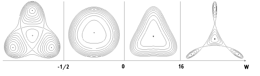
Figure 1: The lines of the level of PES for different structurally stable regions.

The coordinates of critical points are determined by

$$\begin{gathered}\bar{x}_{1}=0,\quad y_{1}=0\hfill\\ \bar{x}_{2,3}=0,\quad y_{2,3}=\frac{{\alpha_{i}}}{8}\left({1\pm\sqrt{1-\frac{{16}}{W}}}\right)\hfill\\ x_{4-7}=\pm\sqrt{3}y_{4-7},\quad y_{4-7}=-\frac{{\alpha_{i}}}{{16}}\left({1\pm\sqrt{1-\frac{{16}}{W}}}\right)\hfill\\ \end{gathered}$$ (27)

where $a_{1}=W,a_{2}=\sqrt{W},a_{3}=1.$

The region of the space of parameters $0<W<16$ includes the potentials possessing the unique extremum - the minimum in the origin of coordinates, corresponding to the spherically symmetric equilibrium shape of nucleus. The region $W>16$ includes the potential surfaces with four minima. The central minimum, with $x=y=0$ , corresponds to the spherically symmetric equilibrium shape of nucleus, but three peripheral minima correspond to deformed shape. At last, in the region $W<0$ $(a<0)$ we run into the potentials, describing the nuclei, which are deformed in the ground state and even don’t have the quasistable spherically symmetric excited state. This region can be divided into two subregions. In the space of parameters the boundary between these subregions $W=-1/2$ represents the geometric locus, where the both eigenvalues of matrix of stability turn into zero simultaneously.

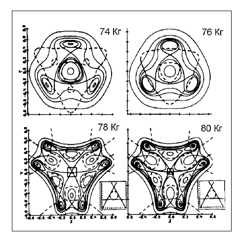
Figure 2: The surfaces of potential energy of Krypton isotopes.

Seiwert,Ramayya and Maruhn [29] restored the parameters of the Hamiltonian of the quadrupole oscillations, including the sixth degree members in deformation for isotopes $Kr^{74,76,78,80}$ . The big experimental values of energy of the first $2^{+}$ - states for nuclei $Kr^{74,76}$ indicate spherical shape of nucleus surface, while the probabilities of the electromagnetic transitions $2^{+}\to 0^{+}$ and very low energies of the first rotational states (recalculating to one and the same number of nucleons, this energy for isotopes $Kr^{74}$ is essentially lower than the lowest from the known energy for nucleus $Pu^{240}$ - $42.8\;kev$ ) imply the possibility of ”superdeformation” [30]. The nonlinear effects, which are connected with the geometry of PES, must be exhibited in the superdeformed nuclei even at the relatively low energies of excitation. The potential surfaces of Krypton isotopes, which are calculated in [29], are presented in Fig.2. As it is seen, the inclusion into the consideration of the highest members of expansion in deformation leads to a considerable complication of the geometry of PES: for all considered Krypton isotopes we run into the PES of complicated topology with many local minima. It’s clear, that in any degree in deformation of the PES $C_{3\nu}$ - symmetry is preserved.

2.3 Critical energy of transition to chaos

If we understand under the stochastization the process of appearance in the system of statistical properties in consequence of local instability, we obtain a tempting possibility of identifying the values of parameters, that lead to the local instability in the system, with the boundary of transition to chaos. Unfortunately, the criteria of the stochasticity of the similar type, i.e. based on the investigation of the local instability, posses the innate lack: the lost of stability of the regular motion does not obligatory leads to chaos. Generally speaking, instead of this the transition to another more complicated type of regular motion is possible. Besides that, the statement, that the local instabilities define the global dynamics of the system is disputed. Separate details of the derivation of the concrete criteria of the stochasticity provoke several objections. In spite of these serious lacks the available experience allows us to state, that the criteria of the similar type in the aggregate with numerical experiment essentially facilitate the analysis of the many-dimensional nonlinear motion.

A large variety of criteria of the stochasticity is based on the direct evaluation of the rate of divergence of the initially close trajectories $\left\{\vec{q}_{1}(t),\vec{p}_{1}(t)\right\}$ and $\left\{\vec{q}_{2}(t),\vec{p}_{2}(t)\right\}$. Linearized equation of motion for a divergence

$$\vec{\xi}\left(t\right)=\vec{q}_{1}\left(t\right)-\vec{q}_{2}\left(t\right),\quad\vec{\eta}\left(t\right)=\vec{p}_{1}\left(t\right)-\vec{p}_{2}\left(t\right)$$ (28)

assume the following form

$$\dot{\vec{\zeta}}(t)=\vec{\eta},\quad\dot{\vec{\eta}}(t)=-\hat{S}(t)\vec{\zeta}$$ (29)

where $\hat{S}(t)$ is a matrix of stability, constructed from the second derivatives of a potential $U(\vec{q})$ and calculated along the support trajectory $\vec{q}_{1}\left(t\right)$

$$S_{ij}\left(t\right)=\left.{\frac{{\partial^{2}U}}{{\partial q_{i}\partial q_{j}}}}\right|_{\overrightarrow{q}=\overrightarrow{q_{1}}\left(t\right)}$$ (30)

The stability of motion of the dynamic system, described by the Hamiltonian

$$H\left({\vec{p},\vec{q}}\right)=\frac{{\vec{p}^{2}}}{2}+U\left({\overrightarrow{q}}\right)$$ (31)

is determined in $N$- dimensional case by $2N\times 2N$ matrix

$$\hat{\Gamma}=\left|{\begin{array}[]{*{20}c}{\hat{O}}&{\hat{I}}\\ {-\hat{S}\left(t\right)}&{\hat{O}}\\ \end{array}}\right|$$ (32)

where $\hat{O}$ and $\hat{I}$ is a zero and a unit$N\times N$ matrices. If even one of the eigenvalues $\lambda_{i}$ of the matrix $\hat{\Gamma}$ is real, then the divergence of the trajectory increases exponentially and the motion is unstable. The imaginary eigenvalues correspond to the stable motion. The eigenvalues, and consequently the character of motion change with the time.

The problem of the investigation of the stable motion can be essentially simplified [31], if we assume the possibility of a replacement time-dependent point of phase space $\overrightarrow{q_{1}}(t)$ by time-independent coordinate $\vec{q}$ . It reduces the equations for variations (29) to a system of autonomous linear differential equations

$$\dot{\vec{\xi}}=\vec{\eta}\quad;\quad\dot{\vec{\eta}}=-\hat{S}\left({\overrightarrow{q}}\right)\overrightarrow{\xi}$$ (33)

An equation for Lyapunov exponents l which determine the character of motion

$$\left|{\det\hat{\Gamma}-\lambda\hat{I}}\right|=0$$ (34)

for the system with two degrees of freedom (the system of our interest) has the following solution

$$\lambda_{1,2,3,4}=\pm\left[{-\beta\pm\sqrt{\beta^{2}-4\gamma}}\right]$$ (35)

where

$$\begin{gathered}\beta=Sp^{\prime}\hat{S}=U_{xx}+U_{yy},\hfill\\ \gamma=\det\hat{S}=U_{xx}U_{yy}-U_{xy}^{2}\hfill\\ \end{gathered}U_{xx}\equiv\frac{{\partial^{2}U}}{{\partial x^{2}}},U_{yy}\equiv\frac{{\partial^{2}U}}{{\partial y^{2}}},U_{xy}\equiv\frac{{\partial^{2}U}}{{\partial x\partial y}}.$$ (36)

Here we will assume that $\beta>0$. Then, providing that $\gamma>0$ , Lyapunov exponents are purely imaginary and the motion is stable. With $\gamma<0$ the pair of roots becomes real and it leads to exponential divergence of close trajectories, i.e. to the instability of motion.

Now let’s remind several known facts from the theory of surfaces [32]. Gaussian curvature of a surface is equal to the ratio of the determinants of the second $\hat{b}$ and the first $\hat{g}$ quadratic forms

$$K=\frac{{b_{11}b_{22}-b_{12}^{2}}}{{g_{11}g_{22}-g_{12}^{2}}}\Rightarrow=\frac{{\det\hat{b}}}{{\det\hat{g}}}$$ (37)

In particular, if the surface is given in the form of the graph $z=U\left({x,y}\right)$ , then

$$\begin{gathered}\det\hat{b}=\frac{{U_{xx}U_{yy}-U_{xy}^{2}}}{{1+U_{x}^{2}+U_{y}^{2}}}\hfill\\ \det\hat{g}=1+U_{x}^{2}+U_{y}^{2}\hfill\\ \end{gathered}$$ (38)

and therefore

$$K\left({x,y}\right)=\frac{{U_{xx}U_{yy}-U_{xy}^{2}}}{{\left({1+U_{x}^{2}+U_{y}^{2}}\right)^{2}}}$$ (39)

The Gaussian curvature $K$ can be represented in the form of the product of the so-called principal curvatures $d_{1}$ and $d_{2}$ , which are the eigenvalues of the pair of the matrices $\hat{b}$ and $\hat{g}$ and are the solutions of the equation

$$\det\left({\hat{b}-\delta\hat{g}}\right)=0$$ (40)

The sum of $d_{1}+d_{2}$ is called an average curvature of the surface. We will enlarge on the geometric sense of the Gaussian curvature. Let’s choose the orthonormalized frame $(x,y,z)$ for given point $x_{0},y_{0}$ of surface, where $z$ axis is a normal to the surface. Then locally the surface will be written as $z=U(x,y)$ and $U_{x}^{\prime}=U_{y}^{\prime}=0$ in this point. Therefore

$$\delta_{1}\delta_{2}=K=U_{xx}U_{yy}-U_{xy}^{2}$$ (41)

We will consider three possible cases

1) $K>0,\delta_{1}>0,\delta_{2}>0$ (minimum of the function $U(x,y)$ with $x=x_{0},y=y_{0}$ ,

2) $K>0,\delta_{1}<0,\delta_{2}<0$ (maximum of the function $U(x,y)$ with $x=x_{{}_{0}},y=y_{0}$ ,

3) $K<0,\delta_{1}<0,\delta_{2}>0$ or vice versa (saddle point of the function $U(x,y)$ with $x=x_{0},y=y_{0}$ .

At $K>0$ the surface is locally situated on one side of tangential plane to the investigating point. At $K<0$ the surface necessarily crosses the tangential plane as close as possible to the point of tangency. If the Gaussian curvature is positive everywhere, then this surface is strictly convex.

Recently, in different sections of physics a definite interest has grown to the surfaces which everywhere possess a negative curvature [33]. Such surfaces in the neighbourhood of any point behave as in the neighbourhood of the hyperbolic singular point. Now let’s return to the expression of Liapunov exponents in the case of two-dimensional potential surfaces. Comparing the (36) and (39) expressions we notice that the g sign coincides with the sign of Gaussian curvature of the PES. This association suggests [34, 35] the possibility of the existence of the following scenario of the transition from regular to chaotic motion, based on the investigation of Gaussian curvature of the PES.

At low energies the motion near the minimum of the potential energy, where the curvature is obviously positive, is periodic or quasiperiodic in character and is separated from the instability region by the zero curvature line. As the energy grows, the ”particle” will stay for some time in the negative-curvature region of the PES where initially close trajectories exponentially diverge. At large time these results in the motion which imitate a random one and is usually called stochastic. According to this stochastization scenario, the critical energy of the transition to chaos, $E_{cr}$ , coincides with the lowest energy on the zero curvature line

$$E_{cr}=U_{\min}(K=0)$$ (42)

In the subsequent discussion we will reference to this statement, as to the negative curvature criterion (NCC) .

Now we shall concentrate our attention on one of the first (1959 year) widely used criterion of transition to chaos, the so-called overlap resonance’s criterion (ORC) [36] (the criterion of Chirikov). The essence of this criterion is easier to explain by the example of one-dimensional Hamiltonian system, which is subjected to monochromatic periodic perturbation. This one is the simplest Hamiltonian system which assumes the chaotic behaviour

$$H=H_{0}\left({p,x}\right)+Fx\cos\Omega t$$ (43)

For unperturbed system we can always introduce the variables action-angle $\left({I,\theta}\right)$ in which

$$H=H_{0}\left(I\right)+\sum\limits_{k=-\infty}^{\infty}{x_{k}\left(I\right)\cos\left({k\theta-\Omega t}\right)}$$ (44)

where

$$x_{k}\left(I\right)=\frac{1}{{2\pi}}\int\limits_{0}^{2\pi}{d\theta e^{ik\theta}x\left({I,\theta}\right)}$$ (45)

In new variables the scenario of stochasticity, on which the overlap resonance’s criterion (ORC) is based on, is the following. An external field which is periodic in time induces a dense set of resonances in the phase space of a nonlinear conservative Hamiltonian system. The positions of these resonances, $I_{k}$ , are determined by the resonance condition between the eigenfrequency $\omega_{k}\left(I\right)=\frac{{\partial H_{0}}}{{\partial I_{k}}}$ and frequency of the external perturbation, $\Omega$ . For very weak external fields the principle resonance zones remain isolated. As the amplitude $F$ of external field is raised, the widths $W_{k}$ of the resonance zones increase

$$W_{k}=\left.{4\left({\frac{{Fx_{k}}}{{\omega^{\prime}\left(I\right)}}}\right)^{{\raise 2.1097pt\hbox{$1$}\!\mathord{\left/{\vphantom{12}}\right.\kern-1.2pt}\!\lower 2.1097pt\hbox{$2$}}}}\right|_{I=I_{k}}$$ (46)

and at $F>F_{cr}$ resonances overlap. When this overlap occurs, i.e. under the condition

$$\frac{1}{2}\left({W_{k}+W_{k+1}}\right)=\left|{I_{k}-I_{k+1}}\right|$$ (47)

it is said that there is transition to a global stochastic behaviour in the corresponding region of the phase space. In other words the ORC postulates, that the last invariant KAM surface, which separates the neighbouring resonances, is destroyed in the moment of contact of unperturbed separatrices of these resonances. In other words , the averaged motion of the system in the neighbourhood of the nonlinear isolated resonance on the plane of the variables action-angle is similar to the particle behavior in the potential well. Several isolated resonances correspond to several isolated potential wells. The overlap of the resonances means, that there is such an approach of the potential wells, wherein the random walk of a particle between these wells is possible.

The outlined scenario can easily be ”corrected” for the description of the transition to chaos in the conservative system with several degrees of freedom. The condition of the resonance between the eigenfrequency and the frequency of external field must be replaced by the condition of the resonance between the frequencies, which correspond to different degrees of freedom

$$\sum{m_{i}\frac{{\partial H_{0}}}{{\partial I_{i}}}=0}$$ (48)

The role of the amplitude of the external field in this case plays the intensity of the interaction between different degrees of freedom , i.e. the measure of nonlinearity of the original Hamiltonian. This parameter is usually the energy of system.

This method must be slightly modified for the systems with the unique resonance. In this case the origin of the large-scale stochasticity is connected [37] with the destruction of the stochastic layer near the separatrix of this unique resonance. The essence of the modification consists in the approximate reduction of the original Hamiltonian in the neighbourhood of resonance to the Hamiltonian of nonlinear pendulum, which interacts with periodic perturbation

$$H\left({v,x,\tau}\right)=\frac{1}{2}v^{2}-M\cos x-P\cos k\left({x-\tau}\right)$$ (49)

The width w of the stochastic layer of the resonance is equal to[38]

$$w\approx{\raise 3.01385pt\hbox{${pe^{-{\raise 2.1097pt\hbox{$1$}\!\mathord{\left/{\vphantom{1\rho}}\right.\kern-1.2pt}\!\lower 2.1097pt\hbox{$\rho$}}}}$}\!\mathord{\left/{\vphantom{{pe^{-{\raise 2.1097pt\hbox{$1$}\!\mathord{\left/{\vphantom{1\rho}}\right.\kern-1.2pt}\!\lower 2.1097pt\hbox{$\rho$}}}}{M\rho^{2k+1}}}}\right.\kern-1.2pt}\!\lower 3.01385pt\hbox{${M\rho^{2k+1}}$}}$$ (50)

where

$$\rho={\raise 3.01385pt\hbox{${2M^{{\raise 2.1097pt\hbox{$1$}\!\mathord{\left/{\vphantom{12}}\right.\kern-1.2pt}\!\lower 2.1097pt\hbox{$2$}}}}$}\!\mathord{\left/{\vphantom{{2M^{{\raise 2.1097pt\hbox{$1$}\!\mathord{\left/{\vphantom{12}}\right.\kern-1.2pt}\!\lower 2.1097pt\hbox{$2$}}}}{\pi k}}}\right.\kern-1.2pt}\!\lower 3.01385pt\hbox{${\pi k}$}}$$ (51)

If $p/M$ has the power $\rho^{S}$ , then

$$w\approx\rho^{-\lambda}e^{-{\raise 2.1097pt\hbox{$1$}\!\mathord{\left/{\vphantom{1\rho}}\right.\kern-1.2pt}\!\lower 2.1097pt\hbox{$\rho$}}}$$ (52)

where

$$\lambda=2k+1-s.$$ (53)

At

$$\rho_{i}=\frac{1}{\lambda}\left[{1-\left({1+\lambda}\right)^{-{\raise 2.1097pt\hbox{$1$}\!\mathord{\left/{\vphantom{12}}\right.\kern-1.2pt}\!\lower 2.1097pt\hbox{$2$}}}}\right]$$ (54)

the function $w(r)$ has a point of inflection. The fast growth of $w$ allows us to determine the thresholds of the destruction of the stochastic layer as a value

$$\rho_{s}=\lambda^{-2}\left[{\left({1+\lambda}\right)^{{\raise 2.1097pt\hbox{$1$}\!\mathord{\left/{\vphantom{12}}\right.\kern-1.2pt}\!\lower 2.1097pt\hbox{$2$}}}-1}\right]^{2}$$ (55)

This value $\rho$ is such that the tangent to the point $\rho_{i}$ of the function $w$ crosses the axis $\rho$ .

All three described criteria of stochasticity will be used below to determine the critical parameters of the transition to chaos.

2.4 Numerical results versus analytical estimations

Now let us turn to the analysis of the solutions of the equations of motion, which are generated by the Hamiltonian (16). As mentioned above in the section 2.2, the geometry of the PES for the regions

I $0<W<16$

II $W>16$

III $W<0(a<0)$

is essentially different. Undoubtedly the specific character of the PES must be manifested in behaviour of the solutions of the equations of motion. Therefore we shall analyze each of the mentioned regions separately. Notice, that parameters of the Hamiltonian $a,b,c$ were estimated in different phenomenological models [39]. They change in such wide limits that for real nuclei parameter $W={\raise 3.01385pt\hbox{${b^{2}}$}\!\mathord{\left/{\vphantom{{b^{2}}{ac}}}\right.\kern-1.2pt}\!\lower 3.01385pt\hbox{${ac}$}}$ can belong to each of the regions I,II,III.

2.4.1 Region $0<W<16$ : potentials with unique extremum

It is the simplest region for the analysis in which good agreement between the boundary of the transition to chaos, observed in numerical experiments and analytical evaluations, can be obtained with the help of the simplest of the criterion of the transition to chaos - the negative curvature criterion. Once more we remind, that according to this criterion the mechanism of the generation of the local instability consists in hit of the particle in the region of negative Gaussian curvature of the PES and critical energy of the transition to chaos coincides with the minimum value of the energy on the zero Gaussian curvature line. The equation of the last one in re-scale coordinates (further, we shall use the third variant of scaling (23)) is

$$\frac{1}{{48W^{2}}}-\frac{{W-4}}{{12W}}\left({\bar{x}^{2}+\bar{y}^{2}}\right)+\left({\bar{x}^{2}+\bar{y}^{2}}\right)^{2}-\left({\bar{x}^{2}\bar{y}-\frac{1}{3}\bar{y}^{3}}\right)=0$$ (56)

and potential energy on the zero curvature line is

$$U^{K=0}\left({\bar{x},\bar{y}}\right)=\frac{1}{{48W^{2}}}-\frac{{W-10}}{{12W}}\left({\bar{x}^{2}+\bar{y}^{2}}\right)+2\left({\bar{x}^{2}+\bar{y}^{2}}\right)^{2}$$ (57)

As it is seen, the zero curvature line conserves the symmetry of the PES (see Fig.3.). Therefore, the minimum of the energy on the zero curvature line must lie either on the straight line $x=0$ or on the straight lines, obtained from it with the help of the transformations of the symmetry of the discrete group $C_{3\nu}$.

Figure 3: Isolines of the PES for $W=13$ . Zero curvature line $K\left({x,y}\right)=0$ (dashed line) is shown on the background of the level lines, the range $K\left({x,y}\right)<0$ is shaded.

At $0<W<4$ Gaussian curvature of the PES is positive everywhere. At $4<W<12$ the subregion of the negative curvature is localized on the straight line (in the plane) $x=0$ in the interval

$$-\frac{1}{4}\left({1+\sqrt{1-\frac{4}{W}}}\right)<\bar{y}<-\frac{1}{4}\left({1-\sqrt{1-\frac{4}{W}}}\right)$$ (58)

and in the subregion $12<W<16$ the negative curvature appears at $\bar{y}>0$ in the interval

$$\frac{1}{{12}}\left({1-\sqrt{1-\frac{{12}}{W}}}\right)<\bar{y}<\frac{1}{{12}}\left({1+\sqrt{1-\frac{{12}}{W}}}\right)$$ (59)

In Fig. 4. the profiles $U\left({\bar{x}=0,\bar{y}}\right)$ of the PES are shown for the three considered subregions, and the intervals of the negative curvature are shaded.

Thus, according to the considered scenario of the stochastization in the subregion $0<W<4$ the motion must remain regular for all energies. According to the (42) in the neighbourhood of the energy

$$E_{cr}=U_{\min}\left({K=0}\right)=U\left({x=0,y_{cr1}}\right),y_{cr1}=-\frac{1}{4}\left({1-\sqrt{1-\frac{4}{W}}}\right)$$ (60)

the transition to the global stochasticity should be expected in the subregion $4<W<12$. Finally, in the sub region $12<W<16$ this transition must be observed in the neighbourhood of the energy

$$E_{cr}=U_{\min}\left({K=0}\right)=U\left({x=0,y_{cr2}}\right),y_{cr2}=\frac{1}{{12}}\left({1-\sqrt{1-\frac{{12}}{W}}}\right)$$ (61)

In this case we have used that for all $12<W<16$ $U(x=0,y_{cr1})>U(x=0,y_{cr2})$ .

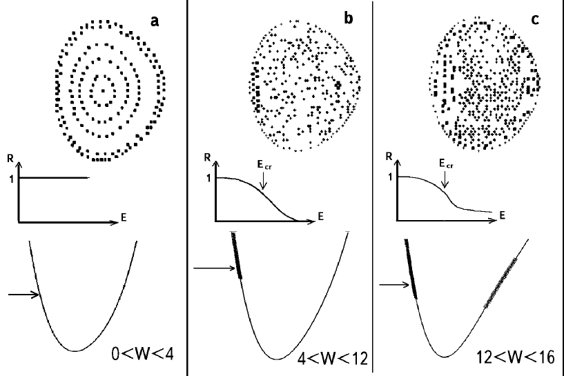
Figure 4: The profiles $U\left({\bar{x}=0,\bar{y}}\right)$ of the PES for the sub regions $0<W<4,\;4<W<12$ and $12<W<16$ . The regions of the negative curvature are shaded. In the top part of the Figure - the Poincare surfaces of section for the energy values indicated by arrows, are represented.

These predictions must be compared with the numerical solutions of the equations of motion generated by the Hamiltonian (22).

Perhaps, the simplest numerical method of the detection of stochasticity is the analysis of the Poincare surfaces of section. As it is well known [40] the Hamiltonian system with $N$ degrees of freedom is integrable only in the case of the existence of $N$ independent univalent integrals of motion. If the number of the integrals of motion is less than the number of degrees of freedom, then the dynamic chaos is possible in the system. In the case of the existence of one or more additional (except energy) integrals of motion, the points of intersection of the phase trajectory with the arbitrary chosen plane (it is just Poincare surface of section) lie on the variety, the dimension of which is smaller than $2N-2$ . Otherwise they will fill all the $2N-2$ dimensional isoenergetic volume (all $2N-2$ isoenergetic surface). Therefore the analysis of the Poincare surfaces of section allows us to establish the fact of the existence of the additional integrals of motion and, consequently, to elucidate which type of motion is realized in the system with the given initial condition. The analysis of Poincare surfaces of section is especially effective for the system with two degrees of freedom, the phase space of which is four-dimensional. In view of the conservation of energy, the trajectory of the particle lies on three-dimensional surface $H\left({p_{x},p_{y},x,y}\right)=const$ . Excepted one of the variables, for example $p_{x}$ , we shall consider the points of intersection of phase trajectory with the plane $x=0$ . In common case they will be chaotic distributed on some part of the plane$(p_{y},y)$ restricted by separatrix. In the case of existence of the additional integral of motion $I\left({p_{x},p_{y},x,y}\right)=const$ the totality of the consecutive intersections with the chosen plane lies on some curve $f(p_{y},y)=const$ . By contrast, chaotic trajectories are identified by the fact that they show no orderly pattern on the Poincare surface of section. As we move from a regular regime into the chaotic one, disorderly trajectories seem to appear first near separatrices between different types of regular orbits. They become visible only in small regions, but as we move further into the chaotic regime, they cover most or almost all of the surface of section until eventually no regular trajectories are visible.

The analysis of Poincare surfaces of section, obtained by the numerical integration of Hamiltonian equations of motion for the PES with unique extremum $(0<W<16)$ , leads to the following results:

1) At low energies $(E<<E_{cr})$ in the neighbourhood of minimum for all considered values $W$ , the motion remains regular. The regularity of the motion with low energies is a straight consequence of the KAM theorem [41, 42], which states, that the majority of the regular trajectories of the unperturbed systems remain regular under sufficiently small perturbation. It is clear that this is accorded with the positiveness of Gaussian curvature in the neighbourhood of any minimum.

2) In the interval $0<W<4$ for all energies the motion remains regular (see Fig. 4a.). This can be explained by the positiveness of the Gaussian curvature of the PES in this region of the parameter $W$ .

3) In the interval $4<W<16$ as the energy increases, the gradual transition from the regular (quasi periodic) motion to chaotic one (see Fig. 4b.) is observed. Moreover in the subregion $4<W<12$ the critical energy, observing in the Poincare surface of section, is close to (60); as in the subregion $12<W<16$ the transition to the global stochasticity is observed in the neighbourhood of the energy, calculated according (61). This effect at $12<W<16$ is connected with the beginning of the region of negative curvature at $y>0$ located below in the energy (see Fig. 4c.).

It is necessary to make one important remark. Analysis of the Poincare surfaces of section allows to introduce the critical energy of the transition to chaos, having determined it as the energy in which the part of phase space with chaotic motion exceeds certain arbitrary chosen value. Similar indetermination is connected with the absence of the sharp transition to chaos for any critical value of the perturbation to which integrated system is undertaken. Therefore a certain caution is required in comparing the ”approximate” critical energy, obtained by any variant of numerical simulation, with the ”exact” value obtained with the help of analytical estimations, i.e. on the base of different criteria of stochasticity.

Based on this remark we can say, that in the case of one-well potentials, the negative curvature criterion allows to make reliable predictions about the possibility of the existence of chaotic regimes in the considered region of the parameters; and also to evaluate the region of energies at which the transition regularity-chaos is performed.

2.4.2 Region $W>16$ : the potentials with a few local minima

Now we are proceeding to the analysis of numerical solutions of the equations of motion in region $W>16$ . The geometry of the PES, which is more complicated in comparison with the potentials which have the unique extremum (see Table 2.2.1), assumes the existence of several energies of the transition to chaos even for the fixed set of parameters of the potential. It means, that for such potentials the so-called mixed states [43] must be observed: at one and the same energy in different minima the various dynamic regimes are realized. The Poincare surfaces of section at different energies for Hamiltonian (22) with $W=18$ are presented in Fig.5. This value $W$ provides equality of depths for the central and peripheral minima. Taking into account $C_{3\nu}$ symmetry of the PES, only one peripheral minimum is presented in this Figure.

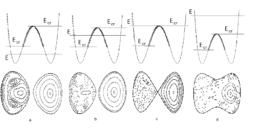
Figure 5: The Poincare surfaces of section for the motion in the potential with $W=18$ at different energies: at the energy less then critical, $E\ll E_{cr}$ , (b) at the energy above critical, $E>E_{cr}$ , (c) at the energy equal to saddle, $E=E_{S}$ .and (d) at the energy above the saddle, $E>E_{S}$ .. The profile $U\left({x=0,y}\right)$ of potential is presented below. The range of $K<0$ is shaded.

The motion represented in Fig. 5.a has clearly defined quasiperiodic character both for the central (left minimum) and for the peripheral (right) minima. Special attention must be given to the distinction in structure of the Poincare surfaces of section for different minima: the complicated structure with several fixed points in left minimum and simple structure with the unique fixed elliptic point in right one. The gradual transition to chaos is observed with the increasing of energy, however the change of the character of motion of the trajectories, localized in certain minimum, is essentially different. Whereas there is the gradual transition to chaos for the left well even for the energy approximately equal to one-half of the saddle energy (Fig. 5.b), and for the energy equal to the saddle one (Fig. 5c), practically all initial conditions correspond to the chaotic trajectories, the motion remains quasi periodic in the (second) right minimum at the same energies. In this minimum the transition to global stochasticity takes place only at the neighbourhood of the saddle energy. In the right well the significant part of phase space corresponding to quasi periodic motion conserves even at the energy essentially exceeding the saddle one (Fig.5d). Figure 6. shows a comparison of the critical energies of the transition to chaos obtained according to the negative curvature criterion and with the help of the analysis of the Poincare surfaces of section. On the base of this comparison we can do the following conclusions.

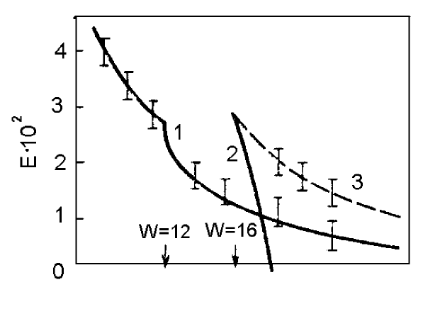
Figure 6: The critical energy of the transition to chaos for region: the negative curvature criterion (rigid line) and with the help of the analysis of the Poincare section.

1) The mixed state is observed for considered potential for region of energies $1/2E_{S}<E<E_{S}(E_{S}-$ saddle energy).

2) The critical energy, defined according to the negative curvature criterion for the left well of potential, is in a good agreement with obtained one by means of numerical integration of the equations of motion and contradicts to the situation for the right well, where the numerical simulation detects large-scale chaos only at attainment of the saddle energy.

The mixed state, which is shown above for the potential of quadrupole oscillations, is the representative state for the wide class of two-dimensional potentials with a few local minima. We shall show this by the example of the polynomial potentials of the degree not higher than six, which are symmetric relatively to the plane $x=0$ . But even with such restrictions, the possible set of the potential forms, depending (generally speaking) on 12 parameters, is too big. Remaining generality, we shall use the methods of the theory of catastrophe [44] in order to reduce amount of calculations. According to the last one, a rather wide class of polynomial potentials with the several local minima is covered by the germs of the lowest umbilical catastrophes, of type $D_{5},D_{4}^{-},D_{7}$ , subjected to the definite perturbations. Let us notice, that the potential of type Henon-Heiles coincides with the elliptic ombilic $D_{4}^{-}$ [44] with precision to linear terms of perturbation.

The mixed state is observed for all considered potentials of umbilical catastrophes in the interval of energies $E_{{}_{cr}}<E<E_{S}$ (here $E_{cr}$ is the critical energy of the transition to chaos determined by negative curvature criterion). The transition to chaos (contrary to the negative curvature criterion) is observed only at the reach of the saddle energy for the minima possessing unique fixed elliptic point in the Poincare surface of section, as in the case of the potential of quadrupole oscillations. This contradiction makes one to refer to the criteria of stochasticity described in the section 2.3., and based on the theory of non-linear resonance.

Let us consider, for example, the Hamiltonian with the PES which represents the germ of the catastrophe $D_{5}$ with quadratic perturbation

$$H=\frac{1}{2}\left({p_{x}^{2}+p_{y}^{2}}\right)+\left[{\frac{1}{4}y^{4}+x^{2}y+ax^{2}-y^{2}}\right]$$ (62)

The geometry of the two-dimensional one-parameter potential $U(x,y;a)$ at $a>\sqrt{2}$ is determined by five critical points : by two minima of equal depth (which thereafter will be named left and right wells) and by three saddles. The energy of the saddle, situated at the origin of the coordinates and separating the wells, does not depend on a and is equal to zero. Therefore, the classical motion will be localized at the separate well at the negative energies. The energies in all the saddles coincide with each other at $a=2$ (this case will be investigated in detail). Now let us estimate the critical energy of the transition to chaos by the negative curvature criterion. In this case the problem is reduced to the search of the conditional extremum - minimum of the potential energy on the zero curvature line. The last one is described by equation

$$\left({y+a}\right)\left({3y^{2}-2}\right)-2x^{2}=0$$ (63)

At $a=2$ we come to the value of the critical energy, which is equal for the both wells

$$E_{cr}=U_{\min}\left({K=0}\right)=-{\raise 3.01385pt\hbox{$5$}\!\mathord{\left/{\vphantom{59}}\right.\kern-1.2pt}\!\lower 3.01385pt\hbox{$9$}}.$$

The results of numerical integration of the equation of motion generated by the Hamiltonian (62) and presented in Fig.7 qualitatively coincide with the results obtained for the Hamiltonian of quadrupole oscillations (Fig.5). Well manifested mixed state is observed at the energies $E\geqslant{\raise 3.01385pt\hbox{$1$}\!\mathord{\left/{\vphantom{12}}\right.\kern-1.2pt}\!\lower 3.01385pt\hbox{$2$}}E_{S}$ in Poincare surfaces of section.

For the explanation of this phenomenon we shall consider the dynamics in the variables angle-action. The Hamiltonian (62) in the system of coordinates with the origin in the left (top sign) and in the right (bottom sign) has the following form

$$H=\frac{1}{2}\left({\dot{x}^{2}+\omega_{1}^{2}x^{2}}\right)+\frac{1}{2}\left({\dot{y}^{2}+\omega_{2}^{2}y^{2}}\right)+x^{2}y\mp\sqrt{2}y^{3}+\frac{1}{4}y^{4}$$ (64)

where $\omega_{1}=\left[{2\left({a\mp\sqrt{2}}\right)}\right]^{{\raise 2.1097pt\hbox{$1$}\!\mathord{\left/{\vphantom{12}}\right.\kern-1.2pt}\!\lower 2.1097pt\hbox{$2$}}},\omega_{2}=2.$

Now we perform the canonical transformation to the variables action-angle of the oscillator part of the Hamiltonian

$$\begin{array}[]{*{20}c}{x=\left({\frac{{2I_{1}}}{{\omega_{1}}}}\right)^{{\raise 2.1097pt\hbox{$1$}\!\mathord{\left/{\vphantom{12}}\right.\kern-1.2pt}\!\lower 2.1097pt\hbox{$2$}}}\cos\varphi_{1},}&{y=\left({\frac{{2I_{2}}}{{\omega_{2}}}}\right)^{{\raise 2.1097pt\hbox{$1$}\!\mathord{\left/{\vphantom{12}}\right.\kern-1.2pt}\!\lower 2.1097pt\hbox{$2$}}}\cos\varphi_{2},}\\ {\dot{x}=\left({2I_{1}\omega_{1}}\right)^{{\raise 2.1097pt\hbox{$1$}\!\mathord{\left/{\vphantom{12}}\right.\kern-1.2pt}\!\lower 2.1097pt\hbox{$2$}}}\cos\varphi_{1},}&{\dot{y}=\left({2I_{2}\omega_{2}}\right)^{{\raise 2.1097pt\hbox{$1$}\!\mathord{\left/{\vphantom{12}}\right.\kern-1.2pt}\!\lower 2.1097pt\hbox{$2$}}}\cos\varphi_{2}.}\\ \end{array}$$ (65)

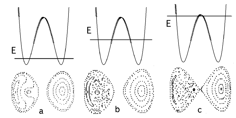
Figure 7: The results of numerical integration of the equation of motion generated by the Hamiltonian with PES which represents the germ of the catastrophe $D_{5}$ with quadratic perturbation (62). In the top part - the profile $U\left({x=0,y}\right)$ of potential. Below - the Poincare surfaces: (a) at the energy less then critical, $E\ll E_{cr}$ , (b) at the energy sligthly above critical, $E>E_{cr}$ and (c) at the energy equal to saddle, $E=E_{S}$ .

In these variables the Hamiltonian (64) has the following form

$$\begin{gathered}H\left({I_{1},I_{2},\varphi_{1},\varphi_{2}}\right)=H_{0}\left({I_{1},I_{2}}\right)+\sum\limits_{m_{1}m_{2}\in y}{f_{m_{1}m_{2}}\left({I_{1},I_{2}}\right)}\cos\left({m_{1}\varphi_{1}+m_{2}\varphi_{2}}\right)\hfill\\ y:\left[{0,1}\right],\left[{0,2}\right],\left[{0,3}\right],\left[{0,4}\right],\left[{2,1}\right],\left[{2,-1}\right]\hfill\\ \end{gathered}$$ (66)

where

$$H_{0}\left({I_{1},I_{2}}\right)=I_{1}\omega_{1}+I_{2}\omega_{2}+\frac{3}{8}\frac{{I_{2}^{2}}}{{\omega_{2}^{2}}}-1$$

$$f_{01}=\frac{{I_{1}}}{{\omega_{1}}}\left({\frac{{2I_{2}}}{{\omega_{2}}}}\right)^{{\raise 2.1097pt\hbox{$1$}\!\mathord{\left/{\vphantom{12}}\right.\kern-1.2pt}\!\lower 2.1097pt\hbox{$2$}}}\pm 3\left({\frac{{I_{2}}}{{\omega_{2}}}}\right)^{{\raise 2.1097pt\hbox{$3$}\!\mathord{\left/{\vphantom{32}}\right.\kern-1.2pt}\!\lower 2.1097pt\hbox{$2$}}}$$

$$f_{02}=\frac{1}{2}\frac{{I_{2}^{2}}}{{\omega_{2}^{2}}},f_{03}=\pm\left({\frac{{I_{2}}}{{\omega_{2}}}}\right)^{{\raise 2.1097pt\hbox{$3$}\!\mathord{\left/{\vphantom{32}}\right.\kern-1.2pt}\!\lower 2.1097pt\hbox{$2$}}}$$

$$f_{04}=\frac{1}{8}\frac{{I_{2}^{2}}}{{\omega_{2}^{2}}},f_{21}=f_{2,-1}=\frac{1}{2}\frac{{I_{1}}}{{\omega_{1}}}\left({\frac{{2I_{2}}}{{\omega_{2}}}}\right)^{{\raise 2.1097pt\hbox{$1$}\!\mathord{\left/{\vphantom{12}}\right.\kern-1.2pt}\!\lower 2.1097pt\hbox{$2$}}}$$ (67)

The term with indexes $r=(r_{1},r_{2})$ is called the resonance term for the given value of energy $E$ , if there are variables action $\left({I_{1}^{r},I_{2}^{r}}\right)$ such that $E=H_{0}\left({I_{1}^{r},I_{2}^{r}}\right)$ :

$$r_{1}\bar{\omega}_{1}\left({I_{1}^{r},I_{2}^{r}}\right)+r_{2}\bar{\omega}_{2}\left({I_{1}^{r},I_{2}^{r}}\right)=0$$ (68)

where

$$\bar{\omega}_{i}={\raise 3.01385pt\hbox{${\partial H_{0}}$}\!\mathord{\left/{\vphantom{{\partial H_{0}}{\partial I_{i}}}}\right.\kern-1.2pt}\!\lower 3.01385pt\hbox{${\partial I_{i}}$}},i=1,2.$$ (69)

It is possible to avoid problems of ”small dominators” to perform canonical transformation to the new action-angle variables which eliminate the dependence of the angle in the lowest order in small parameter identified with the energy at the energies corresponding to the finite motion $(-1<E<0)$ , if we are situated sufficiently far from the resonance, i.e. for all $m_{1},m_{2},$

$$\left|{m_{1}\bar{\omega}_{1}+m_{2}\bar{\omega}_{2}}\right|\leqslant f_{m_{1}m_{2}}$$ (70)

The result of this procedure is the overdetermination of an integrable part $H_{0}(I_{1},I_{2})$ of the initial Hamiltonian and the extension of the set J members depending on angles. In this situation it is possible to meet one of the following three cases:

1) the resonance terms are, as before, absent in the region of energies of our interest;

2) the unique resonance term appears;

3) several resonance terms appear.

In the first case we perform a new canonical transformation and continue the procedure until we meet the situation 1) or 2). In the second case the critical energy, at which the transition to large-scale stochasticity takes place, can be determined by the destruction stochastic layer method [37], while the overlap resonances criterion can be used [36] for the determination of the critical energy in the third case.

Small detuning near the resonance

$$\left|{m_{1}\bar{\omega}_{1}+m_{2}\bar{\omega}_{2}}\right|\leqslant f_{m_{1}m_{2}}$$ (71)

can be compensated by terms of the highest order obtained with the help of repeated canonical transformation of non-resonance terms. In the case when $a=2$ for the resonance (2,-1) the condition (71) of small detuning is performed and procedure, mentioned above, leads to

$$\begin{gathered}H_{0}=I_{1}\omega_{1}+I_{2}\omega_{2}-1+\frac{3}{8}I_{2}^{2}-\frac{{4\omega_{1}+5}}{{32\omega_{1}^{2}\left({\omega_{1}+1}\right)}}I_{1}^{2}+\hfill\\ +\left[{\pm\frac{{3\sqrt{2}}}{2}-\frac{1}{{\omega_{1}\left({\omega_{1}+1}\right)}}}\right]\frac{{I_{1}I_{2}}}{{8\omega_{1}}}\hfill\\ \end{gathered}$$ (72)

In the left well among terms depending on angles we leave only two terms: the resonance term

$${\raise 3.01385pt\hbox{$1$}\!\mathord{\left/{\vphantom{12}}\right.\kern-1.2pt}\!\lower 3.01385pt\hbox{$2$}}\frac{{I_{1}}}{{\omega_{1}}}\left({\frac{{2I_{2}}}{{\omega_{2}}}}\right)^{{\raise 2.1097pt\hbox{$1$}\!\mathord{\left/{\vphantom{12}}\right.\kern-1.2pt}\!\lower 2.1097pt\hbox{$2$}}}\cos\left({2\varphi_{1}-\varphi_{2}}\right)$$ (73)

and ”swinging” term

$$\frac{{\sqrt{2}}}{{64\omega_{1}}}\left[{\frac{3}{{\omega_{1}+1}}+\frac{1}{{\omega_{1}}}}\right]I_{1}I_{2}\cos\left({2\varphi_{1}-2\varphi_{2}}\right),$$ (74)

the direction $m$ of which is the nearest to the resonance direction r. After that the direct application of the destruction stochastic layer criterion leads to the value of critical energy in the left well $E_{cr}\approx-0.51$ which is in well agreement both with the result of numerical simulation and with the predictions of the negative curvature criterion $(-5/9)$ . Immediate analysis of integrable part of Hamiltonian (72) shows, that in the right well the resonances are absent at negative energies and the transition to large-scale stochasticity is possible only with the reach of saddle energy in the complete correspondence with the numerical results .

We can briefly formulate the main results relating to the definition of critical energy of the transition from regular motion to stochastic one concluding comparison of the results of numerical simulation with the analytical estimates .

1. The critical energy of the transition to chaos consistents well with the predictions of the negative curvature criterion for the PES with unique minimum.

2. The critical energy of the transition to chaos either is equal to the minimal energy on the zero curvature line or coincides with the saddle energy for the PES with few local minima .

3 The mixed state is observed in the interval $U_{\min}\left({K=0}\right)<E<E_{s}$ for the potential with several local minima.

4. The possibility of application of negative curvature criterion (NCC) to the particular local minimum is determined by the structure of the Poincare surface of section: for any local minimum,

2.5 Birkhoff-Gustavson normal form

The structure of the Poincare surfaces of section can be reproduced not resorting to the numerical solution of the equations of motion. For this, let us use the method of treating non separable classical systems that was originally developed by Birkhoff [45] and later was extended by Gustavson [46]. The result, obtained by Birkhoff, is the following: if the given Hamiltonian $H$ , which can be written as a formal power series without constant or linear terms, and such that the quadratic terms can be written as a sum of uncoupled harmonic oscillator terms with incommensurable frequencies, then there is a canonical transformation that transforms original Hamiltonian into a normal form. The normal form is a power series in one-dimensional uncoupled harmonic oscillator Hamiltonian. Birkhoff’s method was applied by Gustavson in order to obtain power series expressions for isolating integrals, and to predict analytically the Poincare surfaces of section for the Henon-Helies system. Since the treated potential had commensurable frequencies, Gustavson had to modify Birkhoff’s method only somewhat.

We shall consider the procedure of the transformation to Birkhoff’s normal form for Hamiltonian which is a power series in coordinates $u$ and momenta $v$ [47]

$$H\left({\vec{u},\vec{v}}\right)=H^{\left(2\right)}\left({\vec{u},\vec{v}}\right)+H^{\left(3\right)}\left({\vec{u},\vec{v}}\right)+...$$ (75)

where $H^{(S)}$ has the form of a homogeneous polynomial of degree $s$:

$$H^{\left(s\right)}\left({\vec{u},\vec{v}}\right)=\sum\limits_{\left|i\right|+\left|j\right|=s}{a_{ij}u^{i}v^{j}s=2,3...}$$

$$u^{i}=u_{1}^{i_{1}}u_{2}^{i_{2}}...u_{N}^{i_{N}}\quad\left|i\right|=i_{1}+i_{2}+...+i_{N}$$ (76)

For systems in which $H^{(2)}$ is positive definite, then there exists a canonical transformation $(\vec{u},\vec{v})\to(\vec{q},\vec{p})$ which transforms $H^{(2)}$ into the form

$$H^{\left(2\right)}\left({\vec{q},\vec{p}}\right)=\sum\limits_{k=1}^{N}{\frac{1}{2}\omega_{k}\left({q_{k}^{2}+p_{k}^{2}}\right)}$$ (77)

Let $H(\vec{q},\vec{p})$ be Hamiltonian with $H^{(2)}(\vec{q},\vec{p})$ as given in eq. (77). Then we say that $H(\vec{q},\vec{p})$ is in a normal form, if

$$DH\left({\vec{q},\vec{p}}\right)=0$$ (78)

where

$$D=-\sum\limits_{k}{\omega_{k}\left({q_{k}\frac{\partial}{{\partial p_{k}}}-p_{k}\frac{\partial}{{\partial q_{k}}}}\right)}$$ (79)

This is equivalent to the requiring that the Poisson bracket of $H^{(2)}$ with $H$ vanish, since $D$ is given by

$$D=-\left[{H^{\left(2\right)},}\right]$$ (80)

A power series Hamiltonian can be transformed to the normal form by a sequence of canonical transformations, where each one reduces the non normalized term of the lowest degree to the normal form. The generating function, necessary for the performance of individual transformation, is defined by

$$F\left({\vec{P},\vec{q}}\right)=\sum\limits_{k}{P_{k}q_{k}+W^{\left(s\right)}\left({\vec{P},\vec{q}}\right)}$$ (81)

The connection between old $(\vec{p},\vec{q})$ and new $(\vec{P},\vec{Q})$ canonical variables is

$$Q_{k}=q_{k}+\frac{{\partial W^{\left(s\right)}}}{{\partial P_{k}}},\quad p_{k}=P_{k}+\frac{{\partial W^{\left(s\right)}}}{{\partial q_{k}}},\quad H\left({\vec{p},\vec{q}}\right)=\Gamma\left({\vec{P},\vec{Q}}\right)$$ (82)

where $\Gamma(\vec{P},\vec{Q})$ is the Hamiltonian in the new variables. If we expand $H$ and $\Gamma$ in a Taylor series about $\vec{P}$ and $\vec{q}$ , and then collect and equate all terms of equal degree, the following equation for $W^{(S)}$ is obtained

$$DW^{\left(s\right)}\left({P,q}\right)=\Gamma^{\left(s\right)}\left({P,q}\right)-H^{\left(s\right)}\left({P,q}\right)$$ (83)

In order to solve eq. (83) for $W^{(S)}$ , we make a transformation to variables in which $D$ is diagonal:

$$\begin{gathered}P_{k}=2^{-{\raise 2.1097pt\hbox{$1$}\!\mathord{\left/{\vphantom{12}}\right.\kern-1.2pt}\!\lower 2.1097pt\hbox{$2$}}}\left({\eta_{k}+i\xi_{k}}\right)\hfill\\ q_{k}=i2^{{\raise 2.1097pt\hbox{$1$}\!\mathord{\left/{\vphantom{12}}\right.\kern-1.2pt}\!\lower 2.1097pt\hbox{$2$}}}\left({\eta_{k}-i\xi_{k}}\right)\hfill\\ \end{gathered}$$ (84)

Under this transformation $D\to\tilde{D}$ , where

$$\tilde{D}=i\sum\limits_{k}{\omega_{k}\left({\xi_{k}\frac{\partial}{{\partial\xi_{k}}}-\eta_{k}\frac{\partial}{{\partial\eta_{k}}}}\right)}$$ (85)

It follows that functions of the form

$$\Phi_{l_{1}l_{2}m_{1}m_{2}}\equiv\eta_{1}^{l_{1}}\eta_{2}^{l_{2}}\xi_{1}^{m_{1}}\xi_{2}^{m_{2}}$$ (86)

are the eigenfunction of $\tilde{D}$ , i.e.

$$\tilde{D}\Phi_{l_{1}l_{2}m_{1}m_{2}}=\left[{i\sum\limits_{k}{\omega_{k}\left({m_{k}-l_{k}}\right)}}\right]\Phi_{l_{1}l_{2}m_{1}m_{2}}$$ (87)

Consequently,

$$\tilde{D}^{-1}\Phi_{l_{1}l_{2}m_{1}m_{2}}=\left[{i\sum\limits_{k}{\omega_{k}\left({m_{k}-l_{k}}\right)}}\right]^{-1}\Phi_{l_{1}l_{2}m_{1}m_{2}}$$ (88)

Now the equation (83) may be solved for $\tilde{W}^{(S)}$

$$\tilde{W}^{\left(S\right)}=\tilde{D}^{-1}\left({\tilde{\Gamma}^{\left(S\right)}-\tilde{H}^{\left(S\right)}}\right)$$ (89)

Here $\tilde{H}^{\left(S\right)}$ is a known function. However, so far, $\tilde{\Gamma}^{\left(S\right)}$ has been unspecified. Now $\tilde{\Gamma}^{(S)}$ is determined from the requirement that $\tilde{W}^{\left(S\right)}$ is finite. Clearly, $\tilde{\Gamma}^{(S)}$ must be chosen so that to exactly cancel any terms in $\tilde{H}^{\left(S\right)}$ , which would give a vanishing dominator in eq.(88). So long as the frequencies are incommensurable, the only terms that must appear in $\tilde{\Gamma}^{\left(S\right)}$ are those for which $m_{k}=l_{k}$ for all $k$ ; those terms are

$$\left({i\eta_{1}\xi_{1}}\right)^{m_{1}}\left({i\eta_{2}\xi_{2}}\right)^{m_{2}}=\left[{\frac{1}{2}\left({P_{1}^{2}+q_{1}^{2}}\right)}\right]^{m_{1}}\left[{\frac{1}{2}\left({P_{2}^{2}+q_{2}^{2}}\right)}\right]^{m_{2}}$$ (90)

Such terms are called null space terms, and the remaining terms are called range space terms. Therefore, if $\tilde{H}^{\left(S\right)}$ is separated into null space terms $\tilde{N}^{\left(S\right)}$ and range space terms $\tilde{R}^{\left(S\right)}$ ,

$$\tilde{H}^{(S)}=\tilde{N}^{(S)}+\tilde{R}^{(S)}$$ (91)

and if we require $\tilde{\Gamma}^{(S)}$ to cancel the null space term in $\tilde{H}^{\left(s\right)}$ , eq(89) results in

$$\begin{gathered}\tilde{\Gamma}^{\left(S\right)}=\tilde{N}^{\left(S\right)}\hfill\\ \tilde{W}^{\left(S\right)}=D^{-1}\tilde{R}^{\left(S\right)}\hfill\\ \end{gathered}$$ (92)

In order to make this solution the unique one, it is sufficient to require the generating function containing no null space terms.

If the transformation to Birkhoff’s normal form is made, the harmonic oscillator terms can be transformed to action variables via the canonical transformation (65).

We cite as an example the normal form (up to $s=6$ ) for the Hamiltonian (62) at $a=2$ in the neighbourhood of right minimum

$$\begin{gathered}H\left({I_{1},I_{2}}\right)=2.613I_{1}+2I_{2}-0.219I_{1}I_{2}-0.017I_{1}^{2}-0.375I_{2}^{2}-\hfill\\ -0.005I_{1}^{3}-0.028I_{1}^{2}I_{2}-0.122I_{1}I_{2}^{2}-0.133I_{2}^{3}\hfill\\ \end{gathered}$$ (93)

The commensurability of frequencies results into the extension of the set of null space terms. As a matter of fact

$$\tilde{D}\eta_{1}^{m_{1}}\xi_{2}^{m_{2}}=i\left({m_{1}\omega_{1}-m_{2}\omega_{2}}\right)\eta_{1}^{m_{1}}\xi_{2}^{m_{2}}$$ (94)

and at the realization of condition

$$\left({m_{1}\omega_{1}-m_{2}\omega_{2}}\right)=0$$ (95)

$\tilde{D}^{-1}\eta_{1}^{m_{1}}\xi_{2}^{m_{2}}$ would diverge. In order to avoid this occurrence, $\tilde{\Gamma}^{\left(S\right)}$ must be chosen to cancel any such additional terms in $\tilde{H}^{\left(S\right)}$ . Aside from this change, the procedure is identical to that for the incommensurable case.

The reduction of Hamiltonian to the normal form solves the question about the construction of full set of approximate integrals of motion. The latter can be found by transformation of the variables of action to initial variables. The solution of equations

$$\begin{gathered}H\left({p_{x},p_{y},x,y}\right)=E\hfill\\ I\left({p_{x},p_{y},x,y}\right)=I_{0}\hfill\\ x=const\hfill\\ \end{gathered}$$ (96)

allows to find the set of intersections of phase trajectory with selected plane ($x=const$ ) and by doing so to reconstruct the structure of the Poincare surfaces of section.

The Poincare surfaces of section for the quadrupole oscillations of nuclei $Kr^{74}$ , which are constructed in such a way are shown in Fig.8. The Hamiltonian, describing these oscillations, up to the terms of the sixth degree with the respect to deformation is the following

$$\begin{gathered}H=\frac{1}{2}\left({p_{x}^{2}+p_{y}^{2}}\right)+U\left({x,y}\right)\hfill\\ U\left({x,y}\right)=\frac{a}{2}\left({x^{2}+y^{2}}\right)+b\left({x^{2}y-\frac{1}{3}y^{3}}\right)+c\left({x^{2}+y^{2}}\right)^{2}+\hfill\\ d\left({x^{2}y-\frac{1}{3}y^{3}}\right)\left({x^{2}+y^{2}}\right)+e\left({x^{2}y-\frac{1}{3}y^{3}}\right)^{2}+f\left({x^{2}+y^{2}}\right)^{3}\hfill\\ \end{gathered}$$ (97)

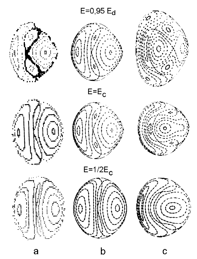
Figure 8: The Poincare surfaces of section for different values of energy for the central minimum of $Kr^{74}$ . a) obtained by the numerical integration of equations of motion; b) obtained with the help of normal forms; c) for the equivalent potential of quadrupole oscillations of the fourth degree.

The parameters determining the dynamics of the particular nucleus, is calculated for the isotopes of Krypton in paper [29]. The Poincare surfaces of section for the equivalent quartic potential, the parameters of which are selected from the condition of coincidence of the situation of critical points and the values of energy in them are shown in the same figure.

2.6 Regularity-chaos-regularity transition

The transition regularity-chaos for nonintegrable low-dimensional Hamiltonian, which is going on as the energy or the amplitude of external field increases, is a well-investigated process. The critical energy of this transition, calculated within the framework of different scenarios of stochastization, at least for potentials with the simple geometry, is in the agreement with the results of numerical simulation. For the systems with localized region of instability (region of negative Gaussian curvature or region of overlap of non-linear resonances) at further increasing of energy, one would expect the return to the regular motion; and the critical energy of this new transition chaos-regularity $E_{cr2}$ will be determined by the top boundary of region of instability. For the Hamiltonian of quadrupole oscillations (22)

$$E_{cr2}=U\left({x=0,y_{cr2}}\right),y_{cr2}=-\frac{1}{4}\left({1+\sqrt{1-\frac{4}{W}}}\right)$$ (98)

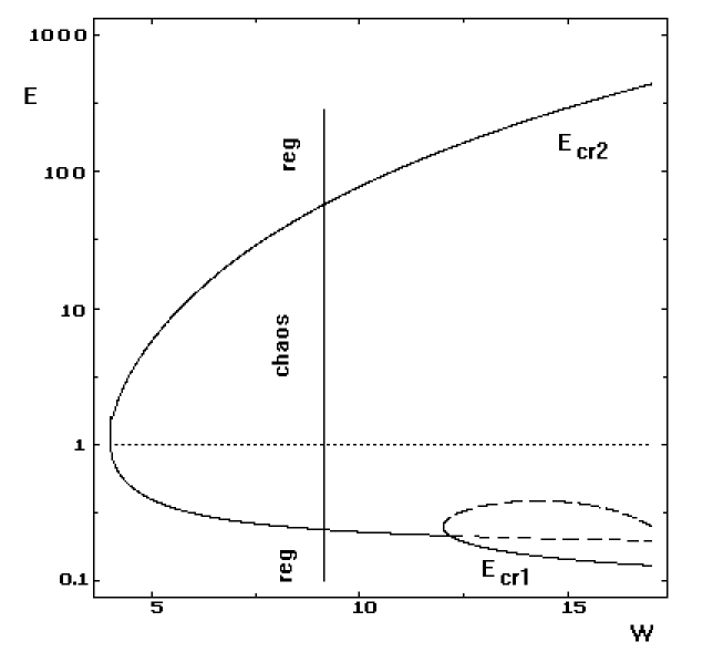
Figure 9: Figure represents ”the phase diagram” that allows to determine energetic intervals of regular and chaotic motions for the fixed value of $W$ . Recall that for the PES with $0<W<4$ at all energies the motion remains regular.

Figure 10: The value of Gaussian curvature $K\left({x=0,y}\right)$ of the PES of $Kr^{74}$ (solid line) and the value of the equivalent potential of the fourth degree (dashed line). The value of $K$ in the shaded range of $y$ are very small (less then 0.1).

Figure 11: The part of phase space $S\%$ .with chaotic traectories as a function of the energy ($E_{S}$ - the saddle energy). The solid line - for potential of isotope $Kr^{74}$ and the dashed line - for equivalent potential of the fourth degree. It is seen that for the nucleus of Krypton the critical energy of the transition chaos-regularity approximately twice exceeds the critical energy for the equivalent potential. With increasing of energy in both potentials the $100\%$ chaos appears. However, at energies considerably exceeded the saddle energy, and for the nucleus $Kr^{74}$ and for the equivalent potential the regular character of motion is restoring.

Recall that for the PES with $0<W<4$ at all energies the motion remains regular. Fig.9 represents ”the phase diagram” that allows to determine energetic intervals of regular and chaotic motions for the fixed value of $W$ .

In the connection with the discussion of possibility of existence of additional transition chaos-regularity, let us trace the change of sign and absolute value of Gaussian curvature for the PES of $Kr^{74}$ (97) and the equivalent PES of the forth degree (16). The parameters of the equivalent PES are fitted according to the condition of coincidence of the position of extremuma of these two potentials and values of energy in them. The value of Gaussian curvature $K(x=0,y)$ of the PES of $Kr^{74}$ and the value of the equivalent potential of the fourth degree are represented in Fig.10. We see, that the region of negative curvature of the PES of the equivalent potential occupies considerably larger region of space and has one order of value larger at $y>0$ than for the PES of $Kr^{74}$ . The measure of divergence of the classical trajectories, which leads to the rise of the stochastic properties in the system, is determined by the size of the region and absolute value of negative Gaussian curvature. This circumstance allows us to understand qualitatively the reason of transition to chaos in nucleus $Kr^{74}$ at comparatively higher energies, than in the equivalent potential: the factors which determine the chaotic character of motion in nucleus $Kr^{74}$ are essentially suppressed. Comparatively small region of space, where the negative Gaussian curvature of the PES of isotope $Kr^{74}$ is localized, determines the character of motion at energies essentially exceeded the saddle energy. The part of chaotic trajectories $S,\%$ in relation to all considered trajectories as a function of energy for the motion in deformation potential of isotope $Kr^{74}$ and equivalent potential of the fourth degree is represented in Fig. 11. It is seen that for the nucleus of Krypton the critical energy of the transition chaos-regularity approximately twice exceeds the critical energy for the equivalent potential. In both potentials the $100\%$ chaos appears with increasing of energy. However, at energies considerably exceeded the saddle energy, and for the nucleus $Kr^{74}$ and for the equivalent potential the regular character of motion is restoring. This new transition chaos-regularity is illustrated by the Poincare surfaces of section at the super higher energies, which are represented in Fig.12.

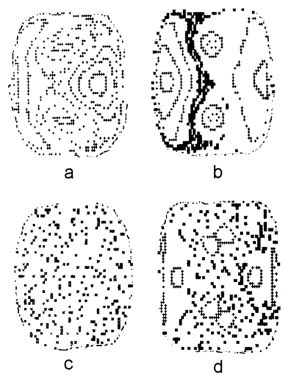
Figure 12: The Poincare surfaces of sections illustrating the restoration regular character of motion at energies considerably exceeded the saddle energy for the nucleus $Kr^{74}$ (b,d) and for the equivalent potential (a,c). The figures (c,d) at the middle energy: $E=100E_{S}$ , and (a,b) - at high energy: $E=1000E_{S}$ .

An earlier appearing of regular motion, at high energies for the quadrupole oscillations of nuclear surface of $Kr^{74}$ comparing with the oscillations in equivalent potential, as with low energies, is explained by smaller absolute value of Gaussian curvature and larger degree of its localization. Underline, that similar reconstruction of regular motion at high energies must occur for any potential with localized region of instability. In particular, it occurs for isotope of $Kr^{76}$ . For isotopes $Kr^{78,80}$ the negative curvature is not spatially localized and that is why the regular character of motion is not reconstructed at energies accessible to numerical calculation.

In conclusion of this section we would like to note the similarity in structure of phase space of considered two-dimensional autonomous Hamiltonian system with the compact region of negative Gaussian curvature and one-dimensional system with periodic perturbation [48].

The behavior of the width of the resonances, $\bar{W}_{k}\equiv\frac{1}{2}\left({W_{k+1}+W_{k}}\right)$ , and the distances between them, $\Delta I_{k}\equiv\left|{I_{k+1}-I_{k}}\right|$ , as a function of the resonance number is the simplest when the satisfaction of resonance overlap condition (2.3.20) for number $k_{1}$ (at a fixed level of the external perturbation) guarantees that this condition holds for arbitrary $k>k_{1}$ . This is precisely the situation which prevails in the extensively studied systems of a $1D$ Coulomb potential [49] and a square well [50] subjected in each case to a monochromatic perturbation. In the former case we have $\bar{W}_{k}\approx k^{{\raise 2.1097pt\hbox{$1$}\!\mathord{\left/{\vphantom{16}}\right.\kern-1.2pt}\!\lower 2.1097pt\hbox{$6$}}}$ and $\Delta I_{k}\approx k^{-{\raise 2.1097pt\hbox{$2$}\!\mathord{\left/{\vphantom{23}}\right.\kern-1.2pt}\!\lower 2.1097pt\hbox{$3$}}}$ , while in the latter we have $\bar{W}_{k}\approx k^{-1}$ and $\Delta I_{k}\approx\left[{k\left({k+1}\right)}\right]^{-1}$ .

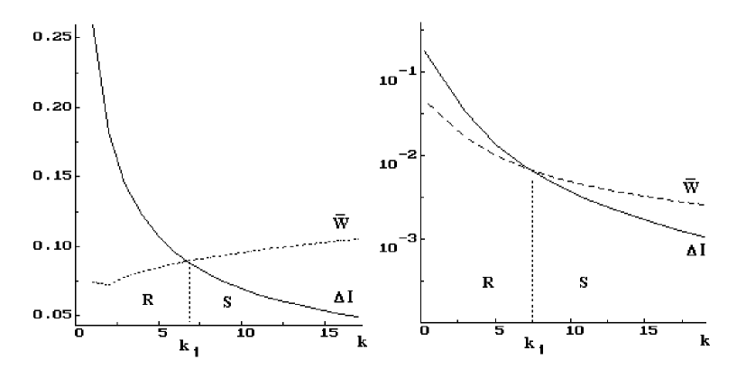
Figure 13: The resonant spacings $\Delta I_{k}$ and the mean widths $\bar{W}_{k}$ as functions of the resonance numbers $k$ . On the left: for one-dimensional Coulomb, on the right: for square-well potential. The critical point $k_{1}$ separates regular range $\left(R\right)$ from the chaotic one $\left(C\right)$ .

As can be seen from Figure 13 there is a regularity-chaos transition (we will call this a ”normal” transition) for both $1D$ Coulomb problem and a square well,since there exists a unique point $k_{1}$ such that at $k>k_{1}$ the condition $\bar{W}_{k}>\Delta I_{k}$ always holds. The motion is therefore chaotic. However, as the behavior of the widths of the resonances and of the distances between them as a function of the resonance number becomes more complex, we can allow the appearance of an additional intersection point and thus a new transition: a chaos-regularity transition, which we will call ”anomalous”. This is also the exotic possibility of the intermittent occurrence of a regular and chaotic regions in the phase space.

We demonstrate that an anomalous chaos-regularity transition occurs in a simple Hamiltonian system: an anharmonic oscillator, subjected to a monochromatic perturbation [48]. The dynamics of such system is generated by the Hamiltonian

$$H\left({p,x,t}\right)=H_{0}\left({p,x}\right)+Fx\cos\Omega t$$ (99)

with the unperturbed Hamiltonian is

$$H_{0}\left({p,x}\right)=\frac{{p^{2}}}{{2m}}+Ax^{n}=E\quad\left({n=2l,l>1}\right)$$ (100)

Considered system fills a gap between two extremely important physical models: the harmonic oscillator ($n=2$ ) and square well ($n=\infty$ ). In terms of action-angle variables $(I,q)$ , the Hamiltonian $H_{0}(p,x)$ becomes

$$H_{0}\left(I\right)=\left({\frac{{2\pi}}{{\alpha G\left(n\right)}}I}\right)^{\alpha}$$ (101)

where

$$G\left(n\right)=\frac{{2\sqrt{2\pi m}\Gamma\left({1+\frac{1}{n}}\right)}}{{A^{{\raise 2.1097pt\hbox{$1$}\!\mathord{\left/{\vphantom{1n}}\right.\kern-1.2pt}\!\lower 2.1097pt\hbox{$n$}}}\Gamma\left({\frac{1}{2}+\frac{1}{n}}\right)}},\alpha=\frac{{2n}}{{n+2}}$$ (102)

The resonant values of the action $I_{k}$ that can be found from the condition $k\omega\left({I_{k}}\right)=\Omega,\quad\omega\left(I\right)=\frac{{dH_{0}}}{{dI}}$ are

$$I_{k}=\alpha\left({\frac{{G\left(n\right)}}{{2\pi}}}\right)^{2n\beta}\left({\frac{\Omega}{k}}\right)^{2n{\raise 2.1097pt\hbox{$\alpha$}\!\mathord{\left/{\vphantom{\alpha\beta}}\right.\kern-1.2pt}\!\lower 2.1097pt\hbox{$\beta$}}},\beta=\frac{1}{{n-2}}$$ (103)

A classical analysis, based on the resonance-overlap criterion, leads to the following expression for the critical amplitude of the external perturbation

$$F_{k}^{cr}=2^{\left({2-3n}\right)\beta}\frac{1}{{4n}}\frac{{\alpha^{2}}}{\beta}\frac{1}{{x_{k}}}\left({\frac{{G\left(n\right)}}{\pi}}\right)^{2n\beta}\Omega^{2n\beta}k^{4\beta}\left[{k^{\left({n+2}\right)\beta}-\left({k+1}\right)^{\left({n+2}\right)\beta}}\right]^{2}$$ (104)

where $x_{k}$ is a Fourier component of the coordinate $x(I,q)$ . Expression (104) solves the problem of reconstructing the structure of the phase space for arbitrary values of the parameters.

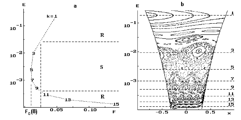
Figure 14: The ”phase diagram” - Figure (a) - the resonance energies $E_{k}$ ($k$ - the resonance number) against the critical values of the external perturbation for Hamiltonian (100). The upper part of curve $\left({k=1-5}\right)$ corresponds to a normal transition regularity-chaos but the lower part of curve $\left({k=5-15}\right)$ corresponds to an anomalous transition chaos-regularity. The snap-shot of $E\left(x\right)$ at the right in Figure (b) confirms that an anomalous chaos-regularity transition occurs. We can clearly see isolated nonlinear resonances that persist at large values of $k$ , and near which the motion remains regular.

The ”phase diagram” in Fig. 14a can be used to determine, at the fixed level of the external perturbation, the energy intervals of regular and chaotic motion. The snap-shot of $E(x)$ at the right in Fig. 14b confirms that an anomalous chaos-regularity transition occurs. We can clearly see isolated nonlinear resonances which persist at large values of $k$ , and near which the motion remains regular. The reason for this anomaly is explained by Fig.15. The plots of the resonance widths and of the distances between resonances in this Figure demonstrate that there are two intersection points $k=k_{1}$ and $k=k_{2}$ , rather than one. Consequently, there is an anomalous chaos-regularity transition.

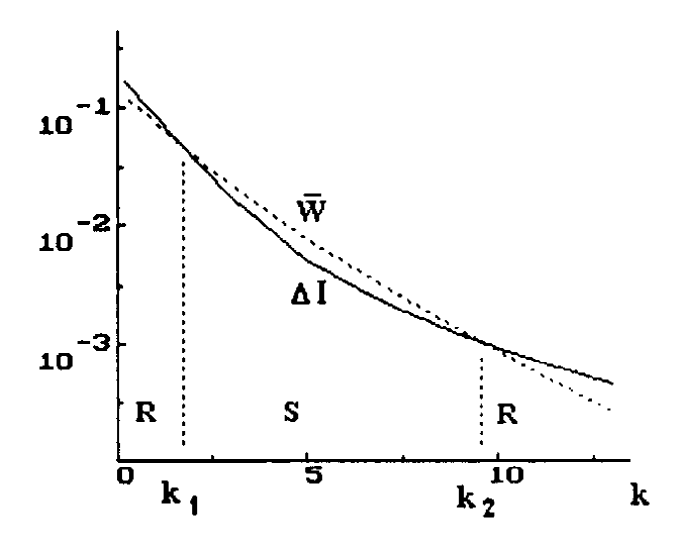
Figure 15: The resonant spacings $\Delta I_{k}$ and the mean widths $\bar{W}_{k}$ as functions of the resonance numbers $k$ for potential (100) with $n=8$ . One can see two critical points $k_{1}$ and $k_{2}$ . The second critical point corresponds to an anomalous chaos regularity transition.

Thus, one can observe the transition regularity-chaos- regularity just as in the case of $2D$ autonomous Hamiltonian system, so in the case of $1D$ system with periodic perturbation. The reason of the additional transition in both cases is common: localized region of instability. In the first case this reason is a localized region of negative Gaussian curvature, in the second one this reason is a localized region of overlap of non-linear resonances.

2.7 Chaotic regimes in reactions with heavy ions

Outlined in the previous sections, the common conception, concerning ossible stochastization of quadrupole nuclear oscillations of high amplitude, is confirmed by the direct observations of chaotic regimes at mathematical simulation of reactions with heavy ions [8].

The time-dependent Hartree-Fock (TDHF) theory [27, 51] constitutes a well-defined starting point for the study of such processes. The TDHF equations can be obtained from the variation of the many-body action $S$ ,

$$S=\int\limits_{t_{1}}^{t_{2}}{dt\left\langle{\Psi\left(t\right)\left|{i\frac{\partial}{{\partial t}}-H}\right|\Psi\left(t\right)}\right\rangle}$$ (105)

In this expression $H$ is the many-body Hamiltonian and the $A$ -nucleon wave function $\Psi(t)$ is chosen to be of determinantal form, constructed from the time-dependent single-particle states $\psi_{\lambda}\left({\vec{r},t}\right)$

$$\Psi\left({\vec{r}_{1},\vec{r}_{2}...\vec{r}_{A};t}\right)=\frac{1}{{\sqrt{A!}}}\det\left\|{\psi_{\lambda}\left({\vec{r},t}\right)}\right\|$$ (106)

The variation of eq.(105) is an independent variation with the respect to the single-particle states $\psi_{\lambda}$ and $\psi_{\lambda}^{*}$ and yields the equations of motion,

$$i\frac{\partial}{{\partial t}}\psi_{\lambda}\left({\vec{r},t}\right)=\frac{{\delta\left\langle H\right\rangle}}{{\delta\psi_{\lambda}^{*}\left({\vec{r},t}\right)}}\equiv h\left({\vec{r},t}\right)\psi_{\lambda}\left({\vec{r},t}\right)$$ (107)

and a similar equation for $\psi_{\lambda}^{*}\left({\vec{r},t}\right)$ .

The classical nature of these equations can be put into a better respective via the definition of classical field coordinates $\phi_{\lambda}\left({\vec{r},t}\right)$ , and conjugate momenta $\pi_{\lambda}\left({\vec{r},t}\right)$

$$\begin{gathered}\phi_{\lambda}={\raise 3.01385pt\hbox{${\left({\psi_{\lambda}+\psi_{\lambda}^{*}}\right)}$}\!\mathord{\left/{\vphantom{{\left({\psi_{\lambda}+\psi_{\lambda}^{*}}\right)}{\sqrt{2}}}}\right.\kern-1.2pt}\!\lower 3.01385pt\hbox{${\sqrt{2}}$}}\hfill\\ \pi_{\lambda}={\raise 3.01385pt\hbox{${\left({\psi_{\lambda}-\psi_{\lambda}^{*}}\right)}$}\!\mathord{\left/{\vphantom{{\left({\psi_{\lambda}-\psi_{\lambda}^{*}}\right)}{\sqrt{2}}}}\right.\kern-1.2pt}\!\lower 3.01385pt\hbox{${\sqrt{2}}$}}\hfill\\ \end{gathered}$$ (108)

Then the result is the Hamiltonian’s equations

$$\begin{gathered}\frac{{d\phi_{\lambda}\left({\vec{r},t}\right)}}{{dt}}=\frac{\begin{gathered}\hfill\\ \delta\left\langle H\right\rangle\hfill\\ \end{gathered}}{{\delta\pi_{\lambda}\left({\vec{r},t}\right)}}\hfill\\ \frac{{d\pi_{\lambda}\left({\vec{r},t}\right)}}{{dt}}=-\frac{{\delta\left\langle H\right\rangle}}{{\delta\phi_{\lambda}\left({\vec{r},t}\right)}}\hfill\\ \end{gathered}$$ (109)

The TDHF equation (107) and its complex conjugate are solved on a three-dimensional space time lattice [52] with initial wave functions of the form

$$\begin{gathered}\lim\phi_{\lambda}\left({\vec{r},t}\right)\to\sqrt{2}\cos\left({\vec{k}_{\lambda}\vec{r}-\varepsilon_{\lambda}t}\right)\chi_{\lambda}\left({\vec{r}}\right)\hfill\\ \lim\pi_{\lambda}\left({\vec{r},t}\right)\to\sqrt{2}\sin\left({\vec{k}_{\lambda}\vec{r}-\varepsilon_{\lambda}t}\right)\chi_{\lambda}\left({\vec{r}}\right)\hfill\\ \end{gathered}$$ (110)

where $\varepsilon_{\lambda}$ is the solution of the static HF equations $h\chi_{\lambda}\left({\vec{r}}\right)=\varepsilon_{\lambda}\chi_{\lambda}\left({\vec{r}}\right)\lambda=1,...A$ and $\vec{k}_{\lambda}$ is the parameter of the initial boost.

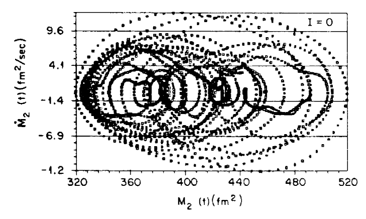
Figure 16: Poincare phases space plot of $\dot{M}_{LI}\left(t\right)vsM_{LI}\left(t\right)$ for isoscalar quadrupole mode for the $Mg^{24}$ system [8].

TDHF calculations for head-on collisions of $He^{4}+C^{14},C^{12}+C^{12}(0^{+}),$ and $He^{4}+Ne^{20}$ have been performed by Umar et. all. [8] at bombarding energies near the Coulomb barrier. The results are interpreted in the terms of their classical behavior. The initial energy and the separation of the centers of the ions are the parameters labeling the initial state. After the initial contact compound nuclear system ($O^{18}$ or $Mg^{24}$ ) relaxes into a configuration, undergoing quasi periodic or chaotic motion. The analysis of nuclear density multipole moments $\left\{{M_{LI}\left(t\right),\dot{M}_{LI}\left(t\right)}\right\}$ has been applied for classifying those solutions Poincare sections. The definitions of the moments are as follows

$$\begin{gathered}M_{LI}\left(t\right)=\int{d^{3}rr^{L}Y_{LM}\left({\hat{r}}\right)}\rho_{I}\left({\vec{r},t}\right)\hfill\\ M_{LI}\left(\omega\right)=\int{dt\exp\left({-i\omega t}\right)M_{LI}}\left(t\right)\hfill\\ \end{gathered}$$ (111)

where isoscalar ($I=0$ ) and isovector ($I=1$ ) densities,

$$\rho_{I}\left({\vec{r},t}\right)=\left\{{\begin{array}[]{*{20}c}{\rho_{p}\left({\vec{r},t}\right)+\rho_{n}\left({\vec{r},t}\right)\quad I=0}\\ {\rho_{p}\left({\vec{r},t}\right)-\rho_{n}\left({\vec{r},t}\right)\quad I=1}\\ \end{array}}\right.$$ (112)

The proton $\rho_{p}$ and neutron $\rho_{n}$ densities in terms of the field coordinates $\phi_{l}$ and momenta $\pi_{l}$ , are

$$\rho_{q}\left({\vec{r},t}\right)=\frac{1}{2}\sum\limits_{\lambda}{\left[{\left|{\pi_{\lambda,q}\left({\vec{r},t}\right)}\right|^{2}+\left|{\phi_{\lambda,q}\left({\vec{r},t}\right)}\right|^{2}}\right],q=p,n}$$ (113)

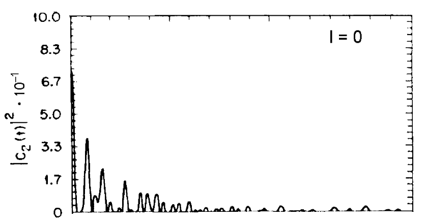
Figure 17: The autocorrelation function $C_{LI}\left(t\right)$ in units $Mev\left({fm^{L}\;\sec}\right)^{2}$ as a function of time for the isoscalar quadrupole mode in the $Mg^{24}$ system [8].

The isoscalar quadrupole mode ($L=2,I=0$ ) is shown in Fig.16 for the $Mg^{24}$ nuclear system seems to be filling most of the available phase space in Poincare section $\left\{{M_{LI}\left(t\right),\dot{M}_{LI}\left(t\right)}\right\}$ . The corresponding autocorrelation function (Fig.17)

$$C_{20}\left(t\right)=\int\limits_{-\infty}^{\infty}{\frac{{d\omega}}{{2\pi}}\exp\left({i\omega t}\right)\left|{M_{20}\left(\omega\right)}\right|^{2}}$$ (114)

damps fast. All this favours the view that corresponding motion is closer to be stochastic rather than quasiperiodic.

3 References