Extended Superscaling of Electron Scattering from Nuclei

1 Introduction

In recent studies [1, 2] the concepts of scaling of the first and second kinds and superscaling have been explored, focusing on the region of energy loss at or below the quasielastic peak in inclusive electron scattering from nuclei. Scaling of the first kind corresponds to the following behavior: if the inclusive cross section is divided by the relevant single-nucleon electromagnetic cross section (i.e., weighted by the proton and neutron numbers, $Z$ and $N$, respectively, and with appropriate relativistic effects included — see [2] for detailed discussions), then at sufficiently high values of the momentum transfer $q$ the result so-obtained becomes a function of a single scaling variable and not independently of $q$ and the energy transfer $\omega$. Various definitions for the scaling variable exist (see, for instance, [2]); however, when $q$ is high enough they are almost always simply functionally related in ways that yield scaling behavior in all cases. Such $q$-independence of the reduced response $F(q,\omega)\to F(\psi)$, where $\psi=\psi(q,\omega)$ is the scaling variable, is called scaling of the first kind. Moreover, motivated by earlier work [4], it has been found that when the typical momentum scale of a given nucleus ${\bar{k}}$ is appropriately incorporated in the definition of the scaling variable and the reduced response is also appropriately scaled, $F(q,\omega)\to f(q,\omega)\equiv{\bar{k}}\times F(q,\omega)$, then a second type of scaling behavior is seen — the result becomes independent of nuclear species. This is called scaling of the second kind. When scaling of both the first and second kinds occurs, one calls the phenomenon superscaling.

The studies undertaken recently [1, 2] demonstrated the quality of the scaling behavior, finding that scaling of the first kind is reasonably good for $\psi<0$ (below the quasielastic peak), that scaling of the second kind is excellent in this region, but that both are violated for $\psi>0$ (above the quasielastic peak). Indeed, the scaling of the first kind has been known for some time to be badly violated in this latter region. The recent analyses showed that so also is scaling of the second kind broken in the $\psi>0$ region, but much less so. Finally, in [2] an initial attempt was made to use the limited information on the separate longitudinal and transverse responses, and hence on the scaling behavior of the respective reduced responses. The former appears to superscale, whereas the dominant scale-breaking effects appear to reside more in the latter.

In the present work we pick up these ideas and extend them. We begin by updating our analysis of the relevant inclusive electron scattering scaling behavior in the $\psi<0$ region, thereby obtaining refined values for the typical nuclear momentum scale (henceforth, as in our previous work which was motivated by the Relativistic Fermi Gas (RFG), called the Fermi momentum $k_{F}$) and for a small energy shift $E_{shift}$ included to have the quasielastic peak occur at the place where the scaling variable is zero. Moreover, we assess the sensitivity of the results to variations in both $k_{F}$ and $E_{shift}$ to provide some idea of how much change in one or both can be tolerated when studying the region where $\psi>0$.

We wish to focus on the scale-breaking effects, especially in the $\psi>0$ region, and accordingly we have isolated the transverse response using our previous approach. Within uncertainties that are unfortunately not as small as is desirable, and only for a limited range of kinematics, it appears that the longitudinal reduced response $f_{L}$ in fact superscales and reasonably satisfies the Coulomb sum rule. We shall assume that this is a universal behavior (for all kinematics and for all nuclei — that is the impact of having superscaling), shall then remove the longitudinal contributions and thereby obtain the transverse reduced response, $f_{T}$. Naturally the uncertainties in knowledge of $f_{L}$ propagate into corresponding uncertainites in $f_{T}$, and given better L/T separations the procedure could be refined. However, it is important to the best of our current ability to isolate the transverse part of the inclusive response as it is the one expected to contain the leading scale-breaking effects [2].

Once $f_{T}$ has been isolated we focus on the region above the quasielastic peak, exploring the scaling behavior of $f_{T}$ as a function of $q$ and $k_{F}$, namely, for first- and second-kind scaling. We further divide our discussions into two regimes, (1) a study of the resonance region where $\Delta$’s and $N^{*}$’s are expected to play an important role along with non-resonant meson production, and (2) a study of the very limited data available in the Deep Inelastic Scattering (DIS) region. Upon seeing that the second-kind scaling behavior is only moderately violated in these regimes, and motivated by the type of analysis performed in studying the EMC effect, we also define an appropriate ratio involving the $f_{T}$’s for a pair of nuclei. This provides a convenient measure of the extent to which scaling of the second kind is or is not respected. Indeed, as we shall see, the ratio is very close to unity from the most negative values of the scaling variable (i.e., far below the quasielastic peak) up through the resonance region. Only in the DIS region does the ratio differ from unity by as much as 25%; for most of the region the results lie typically within about 10% of unity.

The paper is organized as follows: in the next section we briefly summarize the basic scaling formalism, drawing on our previous work [1, 2] where more detailed discussions can be found. In Sec. 3 the updated determinations of $k_{F}$ and $E_{shift}$ are discussed, in Sec. 4 the transverse scaling functions $f_{T}$ are presented and in Sec. 5 the ratios involving pairs of nuclei are introduced. For the last, the discussions are focused on two kinematic regimes, the resonance region in Sec. 5.1 and the DIS region in Sec. 5.2. In the former additional modeling is presented to help in understanding why the ratios differ from unity even by the small amount they do. Finally, in Sec. 6 we summarize our observations and conclusions.

2 Basic Scaling Formalism

We begin by summarizing some of the essential expressions used in previous studies of scaling and superscaling in the quasielastic region. First, using the nucleon mass $m_{N}$ as a scale, it proves useful to introduce dimensionless variables to replace the 3-momentum transfer q and energy transfer $\omega$, namely

$$\lambda \equiv \frac{\displaystyle\omega}{\displaystyle 2m_{N}}$$ (1)

$$\kappa \equiv \frac{\displaystyle{\bf q}}{\displaystyle 2m_{N}}.$$ (2)

The (unpolarized) inclusive electron scattering cross section then depends only on $\kappa=|\mbox{\boldmath$\kappa$}|$, $\lambda$ and the electron scattering angle $\theta_{e}$. The dimensionless 4-momentum transfer squared is given by

$$\tau\equiv|Q^{2}|/4m_{N}^{2}=\kappa^{2}-\lambda^{2},$$ (3)

and $Q^{2}=\omega^{2}-q^{2}<0$ in the conventions used here.

In past work it became apparent that a convenient dimensionless scale in quasielastic electron scattering from nuclei is provided by the ratio of a characteristic nuclear momentum ${\bar{k}}=\sqrt{<k^{2}>}$ to the nucleon mass $m_{N}$. For example, in the Relativistic Fermi Gas (RFG) model the characteristic momentum is the Fermi momentum $k_{F}$ and the dimensionless scale is given by $\eta_{F}$, where

$$\eta_{F}\equiv\frac{\displaystyle k_{F}}{\displaystyle m_{N}}\ll 1,$$ (4)

where typically the Fermi momenta range from as small as 55 MeV/c for deuterium, 200 MeV/c for ⁴He, to as large as about 250 MeV/c for very heavy nuclei, and as a consequence the strong inequality above holds. A corresponding dimensionless energy scale is also useful,

$$\varepsilon_{F}\equiv\sqrt{1+\eta_{F}^{2}}=1+\frac{\displaystyle 1}{\displaystyle 2}\eta_{F}^{2}+\cdots,$$ (5)

where then

$$\xi_{F}\equiv\varepsilon_{F}-1=\frac{\displaystyle 1}{\displaystyle 2}\eta_{F}^{2}+\cdots.$$ (6)

Naturally the RFG is only a first approximation to the nuclear dynamics involved in the quasielastic region and thus the Fermi momenta actually employed — and these are obtained by fitting data as discussed below and in [1, 2] — should really be regarded as effective parameters in the problem. Clearly across the periodic table the densities of nuclei change and this is reflected in the fact that the characteristic momentum scale (here $k_{F}$) should also vary, roughly such that the density is proportional to $k_{F}^{3}$. As a consequence the width of the quasielastic response goes as $k_{F}$.

In past studies of the region at and below the quasielastic peak it has proven to be very useful to introduce scaling variables (see, for example, [3]). In the most familiar approach the $y$-scaling variable is employed and one finds that at high momentum transfers the experimental inclusive cross sections divided by an appropriate single-nucleon cross section scale, i.e., become functions only of $y$ and not independently of the energy or momentum transfer. Such behavior is called scaling of the first kind. Alternatively, again using the RFG for guidance, a dimensionless scaling variable $\psi$ emerges naturally [4, 5]:

$$\psi\equiv\frac{\displaystyle 1}{\displaystyle\sqrt{\xi_{F}}}\frac{\displaystyle\lambda-\tau}{\displaystyle\sqrt{(1+\lambda)\tau+\kappa\sqrt{\tau(\tau+1)}}}.$$ (7)

At the naïve quasielastic peak where $\lambda=\tau$ (which corresponds to $\omega=|Q^{2}|/2m_{N}$) one has $\psi=0$ and finds that the RFG response region is mapped into the range $-1\leq\psi\leq+1$. While appearing at first sight to be quite different, in fact the variables $y$ and $\psi$ are closely related. One can write [2]

$$\psi=\frac{y(E_{s}=0)}{k_{F}}\left[1+{\cal O}(\eta_{F}\psi,y/M_{A-1}^{0})\right],$$ (8)

where $E_{s}$ is the separation energy, the difference between the sum of the nucleon plus ground-state daughter masses and the target ground-state mass. Up to the choice made in making the scaling variable dimensionless by dividing by $k_{F}$ (see below), when $E_{s}$ is set to zero the two variables differ only at order $\eta_{F}$ and order $[M_{A-1}^{0}]^{-1}$, and accordingly when scaling of the first kind occurs in one it is bound to occur in the other, as long as corrections to the leading order expressions are small. In effect, what the conventional $y$-scaling variable does that $\psi$ does not is to take into account the (small) shift in energy embodied in $E_{s}$. The simple relationship begins to fail when large excursions are made away from the QE condition $\psi=0$ — in the present work the full expressions are always used.

From such considerations one sees that an improved phenomenological dimensionless scaling variable can be employed in treatments of superscaling [6], namely one with an empirical shift $E_{shift}$. This was done in previous analyses [1, 2] introducing a dimensionless scaling variable as above,

$$\psi^{\prime}\equiv\frac{\displaystyle 1}{\displaystyle\sqrt{\xi_{F}}}\frac{\displaystyle\lambda^{\prime}-\tau^{\prime}}{\displaystyle\sqrt{(1+\lambda^{\prime})\tau^{\prime}+\kappa\sqrt{\tau^{\prime}(\tau^{\prime}+1)}}},$$ (9)

where $\lambda_{shift}\equiv E_{shift}/2m_{N}$, $\lambda^{\prime}\equiv\lambda-\lambda_{shift}$ and $\tau^{\prime}\equiv\kappa^{2}-\lambda^{\prime 2}$.

After this brief summary of the conventional choices of scaling variables, let us next turn to the scaling functions. We begin with the inclusive electron scattering cross section itself, which may be written in various forms (see also later):

$$d^{2}\sigma/d\Omega_{e}d\omega = {\Sigma}_{L}+{\Sigma}_{T}$$ (10)

$$= \sigma_{M}\left[v_{L}R_{L}(\kappa,\lambda)+v_{T}R_{T}(\kappa,\lambda)\right]$$

$$= \sigma_{M}\left[W_{2}+2W_{1}\tan^{2}\theta_{e}/2)\right],$$

where the familiar electron kinematical factors in this Rosenbluth form are given by

$$v_{L} = \left[\frac{\displaystyle\tau}{\displaystyle\kappa^{2}}\right]^{2}$$

$$v_{T} = \frac{\displaystyle\tau}{\displaystyle 2\kappa^{2}}+\tan^{2}\theta_{e}/2$$ (11)

and the longitudinal (L) and transverse (T) response functions are related to $W_{1,2}$ via

$$R_{T} = 2W_{1}$$

$$R_{L} = \left[\frac{\displaystyle\kappa^{2}}{\displaystyle\tau}\right]^{2}W_{2}-\frac{\displaystyle\kappa^{2}}{\displaystyle\tau}W_{1}.$$ (12)

The strategy in discussing scaling in the quasielastic region is, to the extent that it is possible, to divide out the single-nucleon $eN$ elastic cross leaving only nuclear functions. As discussed in [2, 4, 5], this can be accomplished using the reduced response

$$F(\kappa,\psi)\equiv\frac{\displaystyle d^{2}\sigma/d\Omega_{e}d\omega}{\displaystyle\sigma_{M}\left[v_{L}G_{L}(\kappa,\lambda)+v_{T}G_{T}(\kappa,\lambda)\right]}$$ (13)

for the total cross section, or, when individual L and T contributions are being considered (as they are in part of the present work), using

$$F_{L} \equiv \frac{\displaystyle R_{L}}{\displaystyle G_{L}(\kappa,\lambda)}$$ (14)

$$F_{T} \equiv \frac{\displaystyle R_{T}}{\displaystyle G_{T}(\kappa,\lambda)}.$$ (15)

Here the functions $G_{L,T}$ are given by

$$G_{L}(\kappa,\lambda) = \frac{(\kappa^{2}/\tau)[{\tilde{G}}_{E}^{2}+{\tilde{W}}_{2}\Delta]}{2\kappa[1+\xi_{F}(1+\psi^{2})/2]}$$ (16)

$$G_{T}(\kappa,\lambda) = \frac{2\tau{\tilde{G}}_{M}^{2}+{\tilde{W}}_{2}\Delta}{2\kappa[1+\xi_{F}(1+\psi^{2})/2]}$$ (17)

which involve the function $\Delta$:

$$\Delta = \xi_{F}(1-\psi^{2})\left[\frac{\displaystyle\sqrt{\tau(1+\tau}}{\displaystyle\kappa}+\frac{\displaystyle 1}{\displaystyle 3}\xi_{F}(1-\psi^{2})\frac{\displaystyle\tau}{\displaystyle\kappa^{2}}\right]$$ (18)

$$= \frac{\displaystyle 1}{\displaystyle 2}(1-\psi^{2})\eta_{F}^{2}+{\cal O}[\eta_{F}^{3}].$$

As usual one has

$$\tilde{G}_{E}^{2} \equiv ZG_{Ep}^{2}+NG_{En}^{2}$$

$$\tilde{G}_{M}^{2} \equiv ZG_{Mp}^{2}+NG_{Mn}^{2}$$

$$\tilde{W}_{1} = \tau\tilde{G}_{M}^{2}$$

$$\tilde{W}_{2} = \frac{1}{1+\tau}\left[\tilde{G}_{E}^{2}+\tau\tilde{G}_{M}^{2}\right],$$ (19)

involving the proton and neutron Sachs form factors $G_{Ep,n}$ and $G_{Mp,n}$ weighted by the proton and neutron numbers $Z$ and $N$, respectively.

In the region of the QE peak where $|\psi|$ is small it is a good approximation to set $\Delta$ to zero and to expand the functions $G_{L,T}$ in powers of $\eta_{F}^{2}$, retaining only the lowest-order terms, namely to use

$$G_{L}(\kappa,\lambda) = \frac{\kappa}{2\tau}{\tilde{G}}_{E}^{2}+{\cal O}[\eta_{F}^{2}]$$ (20)

$$G_{T}(\kappa,\lambda) = \frac{\tau}{\kappa}{\tilde{G}}_{M}^{2}+{\cal O}[\eta_{F}^{2}].$$ (21)

While such leading-order expansions in $\eta_{F}^{2}$ are very good when $\eta_{F}\times|\psi|$ is small, they become less so when very large excursions away from the QE peak are made and accordingly in the present work we have always used the full expressions in Eqs. (16–17).

As discussed in [4, 5] the RFG model then yields scaling of the first kind, namely, the $F$’s become functions only of $\psi$ (independent of $\kappa$, that is, of $q$); indeed, as discussed in [1, 2], so do the data when $\psi<0$. Moreover, as also discussed in [1, 2, 4], the RFG model and the data both display scaling of the second kind in that the $F$’s can be made independent of the momentum scale in the problem — that is, independent of $k_{F}$ to the order considered in the expansion in the small dimensionless parameter $\eta_{F}$. This is accomplished by defining

$$f \equiv k_{F}\times F$$ (22)

$$f_{L,T} \equiv k_{F}\times F_{L,T},$$ (23)

namely by making them dimensionless through multiplication by the factor $k_{F}$. Comparing Eq. (8) with the above, we see that the mapping of the $F$’s versus $y$ to the $f$’s versus $\psi$ (or $\psi^{\prime}$) is area-conserving: the dimensionless scaling variables contain a factor $k_{F}^{-1}$, while the scaling functions a factor $k_{F}^{+1}$. In the RFG model the $f$’s display scaling of both the first and second kinds, namely, the display superscaling.

3 Determination of $k_{F}$ and $E_{shift}$

In [1, 2] the approach summarized in the previous section was applied to an analysis of the usable data involving inclusive electron scattering in the region of the quasielastic peak. While medium-energy results were included, the main emphasis in that study was placed on the high-energy results from SLAC and from TJNAF [7]–[23]. And, being the first attempt to explore scaling of the second kind and superscaling, we chose not to perform an extensive search to find the “best” choices of the two parameters involved in the fit, namely, $k_{F}$ and $E_{shift}$, but instead selected values that were “reasonable”. Now, given the success of that previous study and the fact that scaling of the second kind appears to be quite well obeyed in the scaling region ($\psi^{\prime}<0$), we have stronger motivation to produce even better fits and to assess the uncertainties in the fit parameters.

In the next section we shall place our focus on the transverse scaling function $f_{T}$ and it would be desirable to adjust $k_{F}$ and $E_{shift}$ for each nuclear species for this quantity. Unfortunately, in the regime where $\psi^{\prime}\ll 0$, it has not been possible to separate the longitudinal and transverse inclusive responses and thus we are forced to make our fits to the total $f$’s. Our hope is that the parameters obtained from fits to the total are also appropriate for the individual $f_{L,T}$.

The total $f$’s are very sensitive functions of $k_{F}$ in the region where $\psi^{\prime}\ll 0$ and yet it is possible to find values of $k_{F}$ for which the data line up extremely well (see, for instance, the high-$q$/small-$\psi^{\prime}$ data shown below). The $E_{shift}$ dependence is less critical than is that on $k_{F}$; nevertheless, by examining the behavior near the quasielastic peak it is clear that some shift is needed to move the response from the naïve peak value of $\omega=|Q^{2}|/2m_{N}$ ($\lambda=\tau$) to where the data require it to be. In Table 1 we list the parameters obtained from global fits to the data [7]–[23].

Table 1: Adjusted Parameters
Nucleus	$k_{F}$ (MeV/c)	$E_{shift}$ (MeV)
Lithium	165	15
Carbon	228	20
Magnesium	230	25
Aluminum	236	18
Calcium	241	28
Iron	241	23
Nickel	245	30
Tin	245	28
Gold	245	25
Lead	248	31

Clearly the energy shift does not vary too much. Presumably it incorporates the separation energy $E_{s}$, the mean binding energy of nucleons in the nucleus and some global aspects of final-state interactions (for instance, RPA correlations which are known to shift the response slightly). While attempts are being made to account for the values found here, it is not a simple problem to address for the relatively high-energy conditions of most of the current study where relativistic effects are known to be very important, and thus here we limit ourselves to the present phenomenological discussion.

The values of $k_{F}$ found vary monotonically once “typical” nuclei — say, beyond carbon — are reached. It should be understood that the values given here are relative and not absolute: if all values are scaled by a common factor, then equally good scaling of the second kind is obtained. The value of 228 MeV/c for carbon is typical of other studies and so we have used this to normalize the rest. The present fits are done emphasizing the large negative $\psi^{\prime}$ region where “contamination” from pion production, 2p-2h MEC effects, resonances and DIS are thought to be small and where the basic underlying nuclear spectral function is presumably revealed most clearly, in contrast to some previous attempts to determine $k_{F}$ using the entire response region. Interestingly the values found here for heavy nuclei are somewhat smaller than those generally chosen — lead, for example, is sometimes assumed to have $k_{F}\cong$ 265 MeV/c. We believe that the present values are more reliable determinations of the effective $k_{F}$’s. Note also the curious value for lithium, curious because the $k_{F}$ used for ⁴He is 200 MeV/c (see [1, 2]). However, this is easily explained if one assumes that ⁶Li is essentially a deuteron (with $k_{F}=$ 55 MeV/c) plus an alpha-particle. Taking the weighted mean $[\{4\times(200)^{2}+2\times(55)^{2}\}/6]^{1/2}$ gives 166 MeV/c, which is very close to the fit value of 165 MeV/c.

To get some feeling for the sensitivity of the fits in Fig. 1 we show the ratio $f_{Au}/f_{C}$ for data from SLAC taken at $\theta_{e}=$ 16 degrees and incident electron energy $E_{e}=$ 3.6 GeV — for more discussion of the existing data used [7]–[23] see [1, 2]. The top panel in the figure shows that in the region $\psi^{\prime}<0$ the data themselves scatter at roughly the 10% level, i.e., scaling of the second kind for these kinematics is satisfied to roughly the 10% level, which is clearly better than scaling of the first kind (see [1, 2] and figures given below). At positive $\psi^{\prime}$ the ratio moves above unity and constitutes the focus of the discussions later in the present work. In the middle panel the $k_{F}$ of gold has been increased by 10 MeV/c: clearly the fit is very poor in the negative $\psi^{\prime}$ region, indicating that the values of $k_{F}$ given in Table 1 are rather finely determined, namely, to only a few MeV/c. In the bottom panel in the figure, the energy shift used for gold is increased by 10 MeV and again the fit is much worse than the “best-fit” value. So the values of $E_{shift}$ given in the table are good to perhaps a few MeV. Finally, note that, in the large positive $\psi^{\prime}$ region which will be discussed in depth below, the sensitivity to variations in either parameter is much weaker. This stems from the rapid all-off of the responses below $\psi^{\prime}=0$, in contrast to the relatively flat response when $\psi^{\prime}>0$.

4 Transverse Scaling Functions

From our previous analysis [2] we have seen indications that the longitudinal scaling function $f_{L}$ exhibits superscaling behavior, that is, it not only displays scaling behavior of the second kind (as does the total $f$ discussed above), but it has scaling behavior of the first kind. Of course, the regime in which this superscaling has been verified is relatively limited, given the difficulty of separating the longitudinal and transverse response functions. In practice, using the analysis in [24] we have made a fit to the combined set of $f_{L}$-values for the higher momentum transfers where scaling of the first kind is seen to occur. The results are shown in Fig. 2.

To make any further progress on the problem, it is necessary to make an assumption and we do so now: we assume that the so-determined longitudinal scaling function shown in Fig. 2 is universal (i.e., superscaling works). Given this universal $f_{L}$ we can immediately reconstruct the longitudinal cross section for any kinematical condition using the expressions given in Sec. 2,

$$\Sigma_{L}=\frac{1}{k_{F}}f_{L}\sigma_{M}v_{L}G_{L},$$ (24)

from this isolate the transverse part of the cross section,

$$\Sigma_{T}=\frac{d^{2}\sigma}{d\Omega_{e}d\omega}-\Sigma_{L}$$ (25)

and so obtain the transverse scaling function,

$$f_{T}(\psi^{\prime})=\frac{\Sigma_{T}}{\sigma_{M}v_{T}G_{T}}.$$ (26)

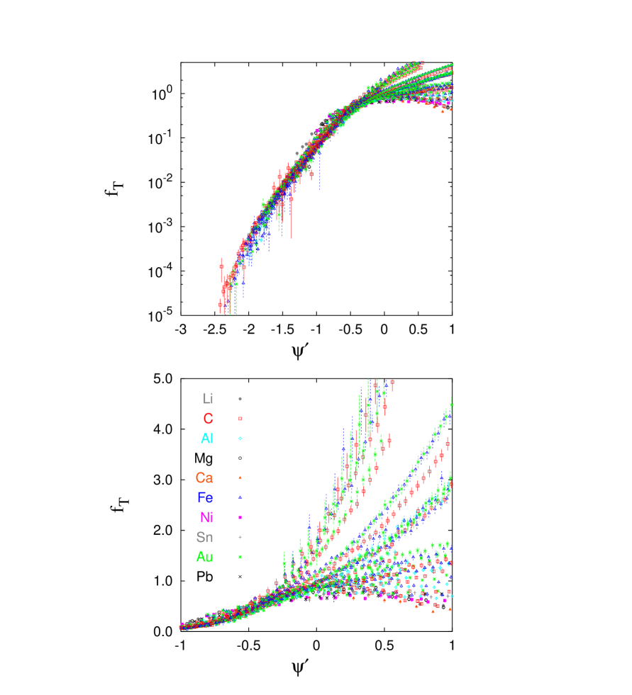
Figure 3: (Color) Transverse scaling function $f_{T}$ for a wide range of nuclei and for kinematics ranging from medium energies (500 MeV and 60 degrees) to high energies (up to 4.045 GeV and 74 degrees). The longitudinal response has been removed using the superscaling assumption discussed in the text. The fit parameters are listed in Table 1.

Using this procedure we arrive at the transverse scaling function $f_{T}$. In Fig. 3 we show the results obtained for all kinematics from medium-energy measurements at 500 MeV and 60 degrees ($q\cong 0.4$ GeV/c) to results from both SLAC and TJNAF ranging up to $q\cong 4$ GeV/c. For $\psi^{\prime}<-0.3$ we see a reasonable convergence of the results to a band, although the width of the band is not negligible, reflecting (at least) breaking of scaling of the first kind. Since the span of momentum transfers is so large in the results shown in the figure, we are emphasizing the lack of 1^st-kind scaling, and focusing on a smaller range of $q$ produces less spread, as discussed below. Note also that the region above $\psi^{\prime}\cong-0.3$ contains a very large spread, that is, a very large degree of scale-breaking. A motivation of the present work is to begin to get some insight into the nature of this behavior.

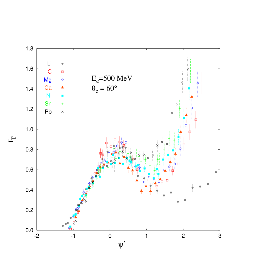
Figure 4: (Color) As in Fig. 3, but only for medium energy data (500 MeV and 60 degrees).

In Fig. 4 we show only the medium-energy results for $f_{T}$. Here, at energy 500 MeV and scattering angle 60 degrees, the momentum transfer varies from about 490 MeV/c at $\psi^{\prime}=-1$ down to about 430 MeV/c at the largest values of $\psi^{\prime}$. We see on the one hand, that now the band in the negative-$\psi^{\prime}$ region is fairly tight, an indication that the breaking seen in Fig. 3 is indeed mainly due to 1^st-kind scale breaking and not to 2^nd-kind breaking. On the other hand, the behavior at positive-$\psi^{\prime}$ shows that there one also has breaking of 2^nd-kind scaling behavior. Clearly as one proceeds from light nuclei with low $k_{F}$ to heavy nuclei with large $k_{F}$ the trend is to increasingly large values of $f_{T}$ in this region. This indicates that the mechanisms that produce the scale-breaking must go as some positive power of $k_{F}$. Indeed, in recent work [25, 26, 27] such breaking of both 1^st- and 2^nd-kinds due to MEC and correlation effects in the 1p-1h sector has been investigated in detail and work is in progress to arrive at a relativistic extension of older work [28] in which scale-breaking in the 2p-2h sector was also identified.

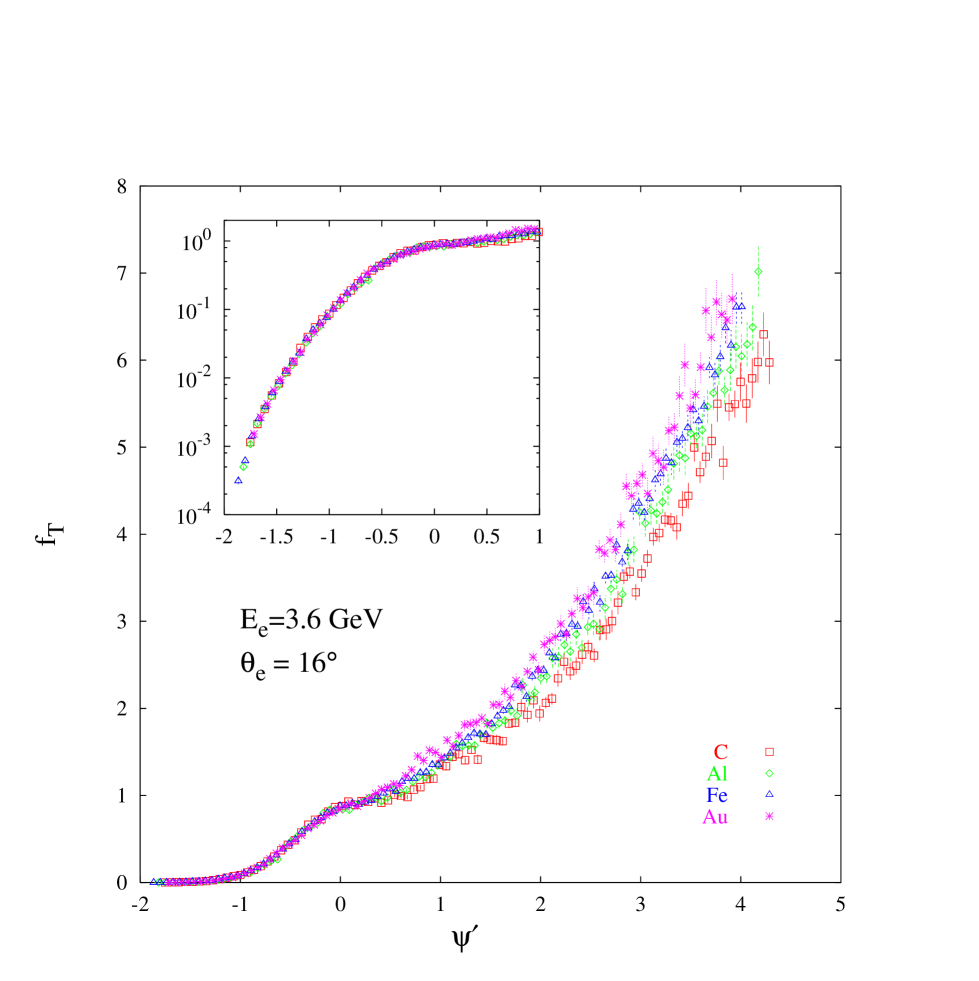
Figure 5: (Color) As in Fig. 3, but only for data at 3.6 GeV and 16 degrees.

Next, in Fig. 5 we show $f_{T}$ for SLAC data at 3.6 GeV and 16 degrees scattering angle. At the lowest values of $\psi^{\prime}$ the momentum transfer is roughly 990 MeV/c while at $\psi^{\prime}\cong 4$ it has risen to about 1.7 GeV/c. As the inset on a semi-log scale clearly shows, the quality of second-kind scaling behavior at higher $q$-values is excellent in the negative-$\psi^{\prime}$ region. At positive $\psi^{\prime}$ 2^nd-kind scaling is not perfect, although it is only modestly broken. The lower the value of $k_{F}$ the smaller is $f_{T}$, indicating again that the scale-breaking mechanisms go as some positive power of $k_{F}$, as expected.

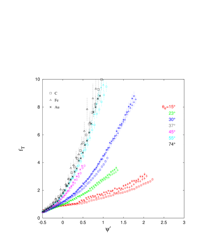
Figure 6: (Color) As in Fig. 3, but for data at 4.045 GeV and angles ranging from 15 to 74 degrees.

Finally, in Fig. 6 we show several sets of data taken at 4 GeV energy and various scattering angles. In this single figure one is able to assess scale-breaking of both kinds. Each fairly tightly-grouped set of data displays the extent of 2^nd-kind scale-breaking and clearly the results are very similar to those already seen in the previous figure. On the other hand, the various scattering angles yield correspondingly different values for the momentum transfer, ranging, for instance at $\psi^{\prime}=+1$ from about 1.2 GeV/c at 15 degrees to 3.9 GeV/c at 74 degrees. For each different choice of kinematics a different grouped set of results is obtained, indicating again the extent to which scaling of the 1^st-kind is broken.

In summary, we deduce from these results for $f_{T}$ that in the region below $\psi^{\prime}\cong 0$ scaling of the 2^nd-kind is excellent, while scaling of the 1^st is violated, although not too badly. In contrast, for $\psi^{\prime}>0$ scaling of the 2^nd-kind is also broken to some extent, whereas scaling of the 1^st-kind is very badly broken. Accordingly, let us next turn to a closer examination of the region above the quasielastic peak to see if further insight can be obtained on how the moderate scale-breaking of the 2^nd-kind arises.

5 Ratios of Transverse Scaling Functions

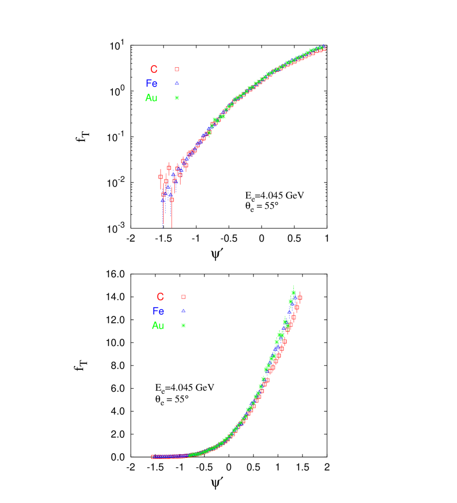
Figure 7: (Color) As in Fig. 6, but only for data at 4.045 GeV and 55 degrees.

The results given in the previous section clearly show that several different regions are involved when studying the first- and second-kind scaling behaviors of $f_{T}$. In the region below the quasielastic peak ($\psi^{\prime}<0$) at high-$q$ the first-kind scaling is reasonably good — this is what is usually called simply $y$-scaling — and the second-kind scaling is excellent. Another example is shown in Fig. 7 containing TJNAF data at 4 GeV and 55 degrees ($q\cong 3.4$–3.5 GeV/c). Clearly one could present the results as a ratio, that is, as $\left[f_{T}(\psi^{\prime})\right]_{2}/\left[f_{T}(\psi^{\prime})\right]_{1}$, where 1 and 2 denote two different nuclei. For $\psi^{\prime}<0$ one would obtain unity with very small uncertainties at all but the lowest values of the scaling variable, while for $\psi^{\prime}>0$ the ratios deviate from unity. In particular, if 1 $\leftrightarrow$ light nucleus and 2 $\leftrightarrow$ heavy nucleus, then the ratio rises above unity in the region above the quasielastic peak. For instance, in Fig. 7 at $\psi^{\prime}=+1$ the Au/C ratio is about 1.2. Thus, even at such high values of the momentum transfer the ratio in the entire region from very large negative $\psi^{\prime}$ to very large positive $\psi^{\prime}$ falls within roughly 20% of unity.

Let us now focus on the region above the quasielastic peak and see if more light can be shed on the remaining (modest, i.e., $\approx$20%) second-kind scale breaking. To begin with, note that the scaling functions $f$, $f_{L}$ and $f_{T}$ have been constructed with the quasielastic responses in mind: the denominator in Eq. (13) contains the elastic eN form factors weighted by $Z$ and $N$, the proton and neutron numbers, respectively. In the region below the quasielastic peak we expect the dominant contributions to the response functions to arise from the tails of the QE response and accordingly removing such a weighted elastic eN cross section makes sense. However, in the region above the quasielastic peak we do not expect things to be so simple. Certainly resonance excitation and pion production play an important role and, at asymptotically high values of momentum transfer, one expects DIS to take over. Because of this one expects the longitudinal and transverse responses to have quite different characters — for instance, the first important new contribution beyond QE scattering in entering the $\psi^{\prime}>0$ region is expected to come from $N\to\Delta$ excitations on nucleons moving in the nucleus, and this is (1) essentially transverse and (2) isovector. For this reason we have extracted the transverse response using the superscaling assumption for the longitudinal contributions. Then, focusing on the transverse results, we can attempt variations on the theme that motivated $y$-scaling in the first place. Specifically, instead of weighting protons and neutrons with $G_{Mp}^{2}$ and $G_{Mn}^{2}$, respectively, we can make a scaling function that varies only with total mass number $A=Z+N$ and not $Z$ and $N$ individually — this is more in the spirit of what is done for the ratio considered when studying the EMC effect. For instance, if an isovector excitation such as $N\to\Delta$ dominates in the response, then equal weighting of protons and neutrons should be better that the weighting provided using the elastic magnetic form factors of the nucleons. Accordingly let us consider

$${\bar{f}}_{T}\equiv\frac{k_{F}\Sigma_{T}}{A\sigma_{M}v_{T}\left(\frac{\tau}{\kappa}\right)G_{D}^{2}},$$ (27)

where $G_{D}$ is the dipole form factor (a compromise between the $Q^{2}$ dependences of $G_{Mp}$ and $G_{Mn}$ — its form is not important here as it will cancel in constructing the ratio defined below). This provides an alternative for $f_{T}$ defined above in Eqs. (15,23). The two differ roughly by a factor

$$\overline{\mu}^{2} \equiv \frac{ZG_{Mp}^{2}+NG_{Mn}^{2}}{AG_{D}^{2}}$$ (28)

$$\cong \frac{Z}{A}\mu_{p}^{2}+\frac{N}{A}\mu_{n}^{2}$$

$$\cong 5.73\left[1-0.36(N-Z)/A\right],$$

which is a relatively slowly-varying function of (Z, N). Such an approximation will allow us to interconnect the quasielastic and DIS analyses in an approximate way (see below).

With these definitions, let us next consider two different nuclei have charge and neutron numbers (Z_i, N_i) with $i=1,$ 2. Labelling as above with nuclear species numbers 1 and 2, we consider the ratio

$$\rho_{12}\equiv\frac{\displaystyle\left[{\bar{f}}_{T}(\psi^{\prime})\right]_{2}}{\displaystyle\left[{\bar{f}}_{T}(\psi^{\prime})\right]_{1}}.$$ (29)

With $\overline{\mu}^{2}_{12}\equiv\overline{\mu_{1}}^{2}/\overline{\mu_{2}}^{2}$ we then have that

$$\frac{\displaystyle\left[f_{T}(\psi^{\prime})\right]_{2}}{\displaystyle\left[f_{T}(\psi^{\prime})\right]_{1}}\cong\overline{\mu}^{2}_{12}\times\rho_{12}\cong\rho_{12},$$ (30)

where the last approximation holds to the degree that

$$\overline{\mu}^{2}_{12}\cong\frac{1-0.36(N_{1}-Z_{1})/A_{1}}{1-0.36(N_{2}-Z_{2})/A_{2}}$$ (31)

is nearly unity across the periodic table. For instance, in going from a nucleus such as carbon ($N_{1}=Z_{1}$) to gold ($N_{2}=118$, $Z_{2}=79$) one has $\overline{\mu}^{2}_{12}\cong 1.08$. Thus the ratio of the $f$’s will be about 8% larger than the quantity $\rho_{12}$ for gold/carbon and even closer to unity for ratios involving nuclei closer together in the periodic table.

From this simple analysis we can see that some of the rise discussed above for the ratio $\left[f_{T}(\psi^{\prime})\right]_{2}/\left[f_{T}(\psi^{\prime})\right]_{1}$ in the region $\psi^{\prime}>0$ occurs because of the different weighting of protons and neutrons in regions dominated by processes other than quasielastic scattering. Two examples of the ratio $\rho_{12}$ are shown in Fig. 8. These have been obtained by extracting the transverse contributions from the experimental cross sections for each nucleus using the superscaling assumption to remove the longitudinal contributions, as discussed in the previous section, calculating ${\bar{f}}_{T}(\psi^{\prime})$ for each nucleus using Eq. (27), fitting the results and finally using Eq. (29) for specific pairs of nuclei. The upper panel in the figure corresponds to momentum transfers of about 1.2 GeV/c (near $\psi^{\prime}=1$) to 1.7 GeV/c (near $\psi^{\prime}=4$), whereas the lower panel ranges from about 2.1 GeV/c (near $\psi^{\prime}=1$) to 2.4 GeV/c (near $\psi^{\prime}=2.5$). Thus, as the momentum transfer grows the ratio seems to stabilize at roughly 5–10% above unity (no error bands are shown in the figure, but typically the uncertainties are $\pm$2%). The analysis in terms of $\rho_{12}$ accounts for some of the 2^nd-kind scale breaking in the region above the quasielastic peak; however, it still does not explain the full effect, but only perhaps half of the 20% discussed above. To get more insight we need to invoke a model of the transverse response in the region $\psi^{\prime}>0$. We proceed in the following two subsections by examining the resonance region and DIS separately.

5.1 In the Resonance Region

Let us begin by focusing on the region in which we expect the excitation of resonances and meson production to become relevant, in addition to the tail of the quasielastic response. In Fig. 8 this corresponds to $\psi^{\prime}\sim 1$–2 (upper panel) and somewhat smaller (lower panel); see below where the scaling variable $\psi_{*}$ is introduced for a more quantitative measure of where a given baryon resonance has its peak. In [29] an extension of the RFG model was discussed. Instead of building the model from elastic scatterings of electrons from nucleons in this work the inelastic $N\to\Delta$ transition was considered and again a relativistic Fermi gas model constructed. Of course the ideas can be extended even further to inelastic excitation of any baryon resonance, that is, with any mass $m_{*}$. Following [29] the RFG hadronic tensor for the production of a stable resonance of this mass is given by

$$W_{\mu\nu} = \frac{\displaystyle 3\pi^{2}{\cal{N}}m_{N}^{2}}{\displaystyle k_{F}^{3}}\int\frac{\displaystyle d\mbox{\boldmath$p$}}{\displaystyle E(\mbox{\boldmath$p$})E_{*}(\mbox{\boldmath$p$}+\mbox{\boldmath$q$})}\theta(k_{F}-p)f_{\mu\nu}(\mbox{\boldmath$p$},\mbox{\boldmath$p$}+\mbox{\boldmath$q$})$$ (32)

$$\qquad\qquad\qquad\times\delta\left[E_{*}(\mbox{\boldmath$p$}+\mbox{\boldmath$q$})-E(\mbox{\boldmath$p$})-\omega\right]\;,$$

where $\cal{N}$ is the number of protons or neutrons (the total nuclear response should be $Z$ times the result for target protons plus $N$ times the result for target neutrons). As usual $E(\mbox{\boldmath$p$})=\sqrt{p^{2}+m_{N}^{2}}$ and now also $E_{*}(\mbox{\boldmath$p$}+\mbox{\boldmath$q$})=\sqrt{(\mbox{\boldmath$p$}+\mbox{\boldmath$q$})^{2}+m_{*}^{2}}$. Here $f_{\mu\nu}$ is the single-nucleon inelastic hadronic tensor:

$$f_{\mu\nu}(\mbox{\boldmath$p$},\mbox{\boldmath$p$}+\mbox{\boldmath$q$}) = -w_{1}(\tau)\left[g_{\mu\nu}-\frac{Q_{\mu}Q_{\nu}}{Q^{2}}\right]$$ (33)

$$+w_{2}(\tau)\frac{1}{m_{N}^{2}}\left[P_{\mu}-\frac{P\cdot Q}{Q^{2}}Q_{\mu}\right]\left[P_{\nu}-\frac{P\cdot Q}{Q^{2}}Q_{\nu}\right],$$

where $w_{1,2}$ are the analogs of $W_{1,2}$ for elastic scattering — the $w$’s for the $N\to\Delta$ case are discussed in [29]; however, for the present purposes it is sufficient simply to know that they are functions only of the 4-momentum transfer $\tau$.

For the strict RFG model one assumes that an on-shell nucleon moving in the initial-state momentum distribution is struck by the virtual photon and an on-shell baryon resonance of mass $m_{*}$ is produced. Of course this is a very over-simplified model (the struck nucleons are not on-shell, the single-nucleon process is not all, the final state is not a stable baryon but a decaying resonant or non-resonant state, etc.), although it does provide some insight into a possible scaling violation mechanism. In particular it can shed some light on when such scale breakings do or do not appear to be very large; that is, it helps to define characteristic kinematic conditions where the QE-type scaling could be expected to evolve into another type of scaling behavior.

Specifically, using the $N\to\Delta$ RFG model of [29] and forming the ratio $\rho_{12}$ defined above one typically obtains results above unity in the $\psi^{\prime}$ region lying between the quasielastic and “$\Delta$” peaks. This is to be compared with the experimental ratio, shown in Fig. 8. For the upper panel in the figure the $N\to\Delta$ RFG peak occurs at $\psi^{\prime}\cong 1.3$ for carbon (1.2 for gold), while for the lower panel the peak occurs at $\psi^{\prime}\cong 0.72$ for carbon (0.67 for gold). The model yields a typical ratio $\rho_{Au/C}$ in the region between the QE and $N\to\Delta$ peaks of approximately 1.08. For the conditions of the lower panel the model yields a ratio that is closer to unity, approximately within 4–5% of unity in the region between the QE and $N\to\Delta$ peaks. Thus we see, even with this over-simplified model, that the remaining few percent deviation from unity of the ratio $\rho_{12}$ is reasonably compatible with resonance production in the $\psi^{\prime}>0$ region corresponding to excitation of the $\Delta$.

Some further insight can be gained about why the ratio behaves as it does by examining some of the specifics of the modeling. In fact, in [29] a scaling variable emerged naturally from consideration of the RFG model for the “$\Delta$” region. Here we generalize this to the scaling variable that occurs in this model for inelastic single-nucleon transitions ($m_{N}\to m_{*}$). With

$$\rho_{*}\equiv 1+\frac{\beta_{*}}{\tau},$$ (34)

where $\beta_{*}\equiv(m_{*}^{2}-m_{N}^{2})/4m_{N}^{2}\geq 0$, we have the analog of Eq. (7):

$$\psi_{*}\equiv\frac{\displaystyle 1}{\displaystyle\sqrt{\xi_{F}}}\frac{\displaystyle\lambda-\tau\rho_{*}}{\displaystyle\sqrt{(1+\lambda\rho_{*})\tau+\kappa\sqrt{\tau(\tau\rho_{*}^{2}+1)}}}.$$ (35)

Futhermore, following the discussions in Sec. 2, one may shift the energy to obtain the analog of Eq. (9),

$$\psi^{\prime}_{*}\equiv\frac{\displaystyle 1}{\displaystyle\sqrt{\xi_{F}}}\frac{\displaystyle\lambda^{\prime}-\tau^{\prime}\rho_{*}^{\prime}}{\displaystyle\sqrt{(1+\lambda^{\prime}\rho_{*}^{\prime})\tau^{\prime}+\kappa\sqrt{\tau^{\prime}(\tau^{\prime}{\rho_{*}^{\prime}}^{2}+1)}}},$$ (36)

where $\rho_{*}^{\prime}\equiv 1+\beta_{*}/\tau^{\prime}$. If $m_{*}=m_{N}$, then $\beta_{*}=0$, which implies that $\rho_{*}=1$ and the above generalized scaling variable yields the standard results in Eqs. (7) and (9). The RFG model for inelastic excitation of a stable resonance of mass $m_{*}$ has scaling behavior of both the first and second kinds in the variable $\psi_{*}$. In particular, if a universal transverse scaling function $f_{T}$ underlies both quasielastic scattering and the excitation of some given resonance from nucleons in the nucleus, then we expect the former to occur in the total transverse cross section as $f_{T}(\psi^{\prime})$ weighted with the usual eN elastic cross section and the latter as $f_{T}(\psi_{*}^{\prime})$ weighted by the N$\to$N^∗ inelastic cross section. Thus we expect (at least) that the scaling behavior involves the way $f_{T}(\psi^{\prime})$ varies with $\psi^{\prime}$ — it scales — versus the way $f_{T}(\psi_{*}^{\prime})$ varies with $\psi^{\prime}$ — note: not how it varies with $\psi_{*}^{\prime}$ in which it scales.

Relationships can be established between $\psi_{*}$ and $\psi$ (or ${\psi_{*}}^{\prime}$ and ${\psi}^{\prime}$ using the primed kinematic variables as above — in the following for simplicity we consider only the unshifted variables):

$$\psi_{*}=\sqrt{1+\gamma_{*}^{2}}\psi-\gamma_{*}\sqrt{\frac{2}{\xi_{F}}+\psi^{2}},$$ (37)

where $2\gamma_{*}^{2}\equiv[(1+\tau)(1+\rho_{*}^{2}\tau)]^{1/2}-(1+\rho_{*}\tau)$. Substituting for $\rho_{*}$ one can write

$$\gamma_{*} = \frac{\beta_{*}}{\sqrt{2\tau(1+\tau)}}\left[\sqrt{\left(1+\frac{\beta_{*}}{1+\tau}\right)^{2}+\frac{1}{\tau}\left(\frac{\beta_{*}}{1+\tau}\right)^{2}}+1+\frac{\beta_{*}}{1+\tau}\right]^{-1/2}$$ (38)

$$\to \frac{\beta_{*}}{2\sqrt{\tau(1+\tau)}},$$ (39)

where the limiting behavior is for $\tau\gg 1$ for fixed $\beta_{*}$ (i.e., fixed $m_{*}$). Under these conditions $\gamma_{*}$ falls as $[\tau(1+\tau)]^{-1/2}$. Thus, if one keeps $m_{*}$ fixed, focusing on a particular resonance, for instance, and examines the behavior of $\psi_{*}$ as a function of $\tau$ and $\psi$ it is clear that as $\tau$ becomes very large $\gamma_{*}\to 0$ and therefore $\psi_{*}\to\psi$, so that there will be no distinction between the two scaling variables. Indeed, to get an idea of how large $\tau$ must be for this to occur, suppose that in addition one has $|\eta_{F}\psi|\ll 1$, then a simple approximation for $\psi_{*}$ is the following:

$$\psi_{*}\cong\psi-\frac{\beta_{*}}{\eta_{F}\sqrt{\tau(1+\tau)}}.$$ (40)

So the value of $\tau$ that characterizes the coalescence of $\psi_{*}$ and $\psi$ is $\tau_{0}=([1+(2\beta_{*}/\eta_{F})^{2}]^{1/2}-1)/2$. For instance, if $m_{*}=m_{\Delta}$ and $k_{F}=230$ MeV/c, then one has $\tau_{0}\cong 0.4$, corresponding to $|Q_{0}^{2}|\cong 1.4\ ($GeV/c$)^{2}$. As the mass of the resonance grows then so does the characteristic $\tau_{0}$, and the coalescence is postponed until larger values of $\tau$.

Given these relationships between the various scaling variables, let us now return to the analysis of 2^nd-kind scale breaking in the resonance region. As noted above we expect some linear combination of $f_{T}(\psi^{\prime})$ and $f_{T}(\psi_{*}^{\prime})$ with weightings according to the elastic and inelastic eN cross sections to be involved in the region between the quasielastic peak ($\psi^{\prime}=0$) and the peak of the specific resonance of interest ($\psi_{*}^{\prime}=0$). As a function of $\psi^{\prime}$ the quasielastic contribution is assumed to exhibit 2^nd-kind scaling, whereas the N$\to$N^∗ contribution does not, because of the dependence on $k_{F}$ in the expressions above. Consider for simplicity the result in Eq. (40). With $\tau$ fixed and considering a given value of $m_{*}$ and hence of $\beta_{*}$ we see that $\psi_{*}$ is less than $\psi$ by the offset $\beta_{*}/[\eta_{F}\sqrt{\tau*(1+\tau)}]$; so $\psi$ is some positive number whereas (being between the QE peak and the resonance peak) $\psi_{*}$ is some negative number. For a small $k_{F}$ the offset is large, whereas for a large $k_{F}$ it is small. That is, for $k_{F}$ small $\psi_{*}$ is further away from zero than when $k_{F}$ is large. Or, said a different way, the difference

$$\psi_{*}(k_{F1})-\psi_{*}(k_{F2})=\frac{\beta_{*}}{\sqrt{\tau*(1+\tau)}}\left[\frac{1}{\eta_{F2}}-\frac{1}{\eta_{F1}}\right]$$ (41)

is positive if $k_{F1}>k_{F2}$, and so $\psi_{*}(k_{F1})$ is closer to zero in this case than is $\psi_{*}(k_{F2})$. Since the inelastic response peaks when $\psi_{*}=0$, this implies that in the region between the QE and N$\to$N^∗ peaks the case with the larger $k_{F}$ should be larger than for the lower-$k_{F}$ case. Indeed this is just what we observe from the data and, in fact, if the offset given above is computed for typical conditions, the degree to which scaling of the 2^nd-kind is broken is found to be quite compatible with those results. These ideas have natural extensions to a distribution of resonances between each of which the same type of phenomenon will occur. The actual magnitude of the effect of course depends on the cross section weighting of each contribution and thus the present arguments should only be regarded as qualitative ones — a more quantitative approach is presently being pursued.

In summary, in effect, the kinematic offset from the QE scaling variable which occurs in the scaling variable that enters naturally when considering baryon excitation from nucleons in the nucleus alone appears to be capable of explaining most of the breaking of 2^nd-kind scaling in the resonance region.

5.2 In the DIS Region

Turning now to the DIS region, let us recall the conventional analysis of $x$-scaling (see, for example, [30]). Noting that the quantity $\nu$ employed in DIS analyses is called $\omega$ in our work, as is usual, and employing the above dimensionless kinematic variables we can write

$$x=\frac{\tau}{\lambda}$$ (42)

and see that when $\psi<0$ we have $x>1$ and the reverse; when $\psi=0$ we have $x=1$.

Using the fact that $x=\tau/\lambda$ one can construct expressions that directly relate $x$ to the scaling variable $\psi$ and Fermi momentum (via $\xi_{F}$) — in particular one useful form is the following:

$$x=\frac{2}{\xi_{F}}\left[\left(\psi+\sqrt{\frac{2}{\xi_{F}}+\psi^{2}}\right)^{2}+\left\{\sqrt{1+\frac{1}{\tau}}-1\right\}2\psi\sqrt{\frac{2}{\xi_{F}}+\psi^{2}}\right]^{-1}.$$ (43)

Or alternatively, if one wishes to work with the Nachtman variable $\xi$ (not to be confused with $\xi_{F}$ used in this and other RFG-motivated studies), then again various useful relationships exist. In particular,

$$\xi = 2(\kappa-\lambda)$$ (44)

$$= \frac{\xi_{F}}{1+\sqrt{1+\frac{1}{\tau}}}\left[\sqrt{\frac{2}{\xi_{F}}+\psi^{2}}-\psi\right]^{2}.$$ (45)

Moreover, it is possible to incorporate the energy shift $E_{shift}$ as above by replacing all quantities on the right-hand sides of Eqs. (43–45) by their primed counterparts to obtain shifted variables $x^{\prime}$ and $\xi^{\prime}$.

Let us examine the $x$-variable a little more closely. As written in Eq. (43) it is a function of $\tau$, $\xi_{F}$ (and hence $k_{F}$) and $\psi$. The last two enter only in the combination $z\equiv\sqrt{\xi_{F}/2}\psi\cong\eta_{F}\psi/2$, since

$$\frac{1}{x}=\left[\sqrt{1+z^{2}}+z\right]^{2}+\left\{\sqrt{1+\frac{1}{\tau}}-1\right\}2z\sqrt{1+z^{2}}.$$ (46)

Thus, as $\tau\to\infty$ one finds that

$$\frac{1}{x}\to\frac{1}{x^{\infty}}\equiv\left[\sqrt{1+z^{2}}+z\right]^{2}.$$ (47)

This behavior holds for $\tau\gg\tau_{crit}$, where, by comparing $x$ with $x^{\infty}$ in the regime where $\psi>0$, one finds that

$$\tau_{crit}=\frac{z\sqrt{1+z^{2}}}{\left[\sqrt{1+z^{2}}+z\right]^{2}}\leq 1/4.$$ (48)

That is, for $|Q^{2}|\gg 1$ (GeV/c)² one has that $x$ is well approximated by $x^{\infty}$. In this regime $x$ becomes a function only of $z$ and thus DIS scaling in $x$ (i.e., independence of $\tau$) and 1^st-kind scaling in $\psi$ will occur together. Furthermore, the above expression for $x^{\infty}$ yields

$$\frac{1}{x^{\infty}} \cong 1+2z\qquad{\rm for\ }\psi\ll\sqrt{2}/\eta_{F}$$ (49)

$$\cong 4z^{2}\ \qquad\quad{\rm for\ }\psi\gg\sqrt{2}/\eta_{F}.$$ (50)

The “asymptotic regime” then occurs when $|Q^{2}|\gg 1$ (GeV/c)² and $x$ is small enough that $\psi\gg\sqrt{2}/\eta_{F}$ (typically $\cong 5$–6), and under these conditions

$$x\rightarrow\frac{1}{\left(\eta_{F}\psi\right)^{2}}.$$ (51)

Thus in the asymptotic regime $x\propto 1/k_{F}^{2}$.

Re-expressing what we have seen in the analyses so far: throughout the region $x>1$, near $x=1$ (essentially the QE peak) and down to about $x=0.3$–0.4 (corresponding to $\psi^{\prime}=3$–4 in Fig. 8) we find that the ratio $\rho_{12}$ is close to unity and that its deviation can be reasonably accounted for by the modest second-kind scale-breaking expected for resonance excitation. Now we wish to explore the higher-$|Q^{2}|$, small-$x$ region in which DIS is expected to be the dominant reaction mechanism.

We begin by providing some “translations” between the nomenclature and conventions employed for most studies done within the context of nuclear physics and those done in particle physics studies. Specifically, what are usually called $\sigma_{L}$ and $\sigma_{T}$ in the latter are given in terms of the responses $W_{1,2}$ and hence via Eqs. (12) of $R_{L,T}$ by the following (here $K$ is an arbitrary factor conventionally taken to be $q$ or sometimes $\omega-\omega(\psi=0)$):

$$\sigma_{T} = \frac{\displaystyle 4\pi^{2}\alpha}{\displaystyle K}W_{1}$$ (52)

$$\sigma_{L} = \frac{\displaystyle 4\pi^{2}\alpha}{\displaystyle K}\left[\frac{\displaystyle\kappa^{2}}{\displaystyle\tau}W_{2}-W_{1}\right].$$ (53)

Their ratio $R$ is then

$$\\ R\equiv\frac{\displaystyle\sigma_{L}}{\displaystyle\sigma_{T}}=\frac{\displaystyle W_{2}}{\displaystyle W_{1}}\left[1+\frac{\displaystyle\lambda^{2}}{\displaystyle\tau}\right]-1,$$ (54)

not to be confused with a different ratio

$${\cal R}\equiv\frac{\displaystyle R_{L}}{\displaystyle R_{T}}=\frac{\displaystyle\kappa^{2}}{\displaystyle 2\tau}R.$$ (55)

As in the previous discussions, we wish, to the degree that we can, to isolate the transverse part of the inclusive cross section. In the DIS regime we must depend on the limited information available for the ratio $R$ defined in Eq. (54) [31, 32]. We then construct

$$\Sigma_{T}=\frac{\sigma}{\left[1+\frac{v_{L}}{v_{T}}{\cal R}\right]}=\frac{\sigma}{\left[1+\frac{v_{L}}{v_{T}}\frac{\kappa^{2}}{2\tau}R\right]}$$ (56)

and from this the transverse scaling function $f_{T}$ and the ratio $\rho_{12}$, as above. In addition to the results shown in Fig. 8 which are not really in the DIS region, we show in Fig. 9 some of the (limited) information available at higher-$|Q^{2}|$ — apparently no information on individual eA cross sections is available at very high momentum transfers and only the usual EMC ratio at constant $x$ has been measured.

Scaling in the DIS regime is usually discussed in terms of the quantities $F_{1}\equiv m_{N}W_{1}$ and $F_{2}\equiv\nu W_{2}$. The so-called EMC ratio is chosen to be $[F_{2}/A]_{2}/[F_{2}/A]_{1}$, where, as above, 1 and 2 label a given pair of nuclei. When this is plotted versus $x$ at very high $|Q^{2}|$ it is seen to be independent of $|Q^{2}|$ and to exhibit the so-called EMC effect. Now our previous analyses and the above discussions show that if one chooses for the abscissa on a plot to use the scaling variable $\psi^{\prime}$, scaled by the Fermi momentum, then one should also incorporate the charge of variables into the ordinate in the plot by multiplying by $k_{F}$. Explicitly this was the procedure used with $\psi^{\prime}\cong y/k_{F}$ (see Eqs. (8,9)) and $f\equiv k_{F}\times F$ (see Eqs. (22,23)). Since here we always display results as functions of $\psi^{\prime}$, we are then motivated also to employ a modified “EMC-type” ratio involving the structure functions for the two nuclear species 1 and 2, but now with factors of $k_{F}$ for each:

$$\rho^{DIS}_{12}\equiv\frac{\left[k_{F}F_{2}/A\right]_{2}}{\left[k_{F}F_{2}/A\right]_{1}}.$$ (57)

Let us now provide the connections between the QE-type ratio and the EMC-type ratio. These may be related via

$$\rho^{DIS}_{12}\equiv X_{12}\rho_{12},$$ (58)

where the factor $X_{12}$ in turn may be decomposed into three factors,

$$X_{12}=R_{12}G_{12}K_{12}.$$ (59)

The first of these,

$$R_{12}=\frac{\displaystyle[1+R]_{2}}{\displaystyle[1+R]_{1}},$$ (60)

arises simply because different parts of the total cross section are conventionally chosen in forming the two ratios. When comparing two different nuclear species at constant $\psi^{\prime}$ it must be remembered that $x$ for species 1 is not the same as $x$ for species 2, but that the two $x$-values are slightly different. In fact, $R_{12}$ is quite close to unity for the range of kinematics under study in this work. The second factor,

$$G_{12}=\frac{\displaystyle[G_{D}^{2}]_{2}}{\displaystyle[G_{D}^{2}]_{1}},$$ (61)

stems from the fact that the QE ratio is defined in Eq. (29) via Eq.(27) to have the typical dipole form factor behavior expected for the transverse part of the elastic eN cross section, whereas the DIS ratio is not — in the latter we expect e-quark scattering to begin to dominate. Again, the fact that we display results versus $\psi^{\prime}$ for experiments where incident electron energy $E_{e}$ and scattering angle $\theta_{e}$ are fixed means that for the two nuclear species the 4-momentum transfers are slightly different. Indeed, $G_{12}$ is typically quite close to unity for the range of kinematics under study. Note that, if sufficient information were available to allow one to specify $|Q^{2}|$, rather than have it vary as here (excepting the case shown in Fig. 9), then this factor would be irrelevant.

The important factor for our purposes is the third one,

$$K_{12}=\frac{\displaystyle\left[\lambda\tau^{2}/\kappa^{3}\right]_{2}}{\displaystyle\left[\lambda\tau^{2}/\kappa^{3}\right]_{1}},$$ (62)

which contains all of the kinematic behavior involved in relating the two types of ratios. At the quasielastic peak this is unity (for simplicity $E_{shift}$ is neglected in these arguments), whereas above the peak it in general differs from unity and so must typically be taken into account. To get some feeling for how it enters in the extreme DIS regime where $\tau\to\infty$ and $x\ll 1$, note that there one has

$$K_{12}^{\infty}=\frac{\displaystyle\left[x^{2}\right]_{2}}{\displaystyle\left[x^{2}\right]_{1}}.$$ (63)

Thus in extreme-DIS kinematics the ratio defined in the present work in Eq. (29) for use in QE scattering differs from the conventional EMC-type ratio essentially by the factor $\left[x^{2}\right]_{2}/\left[x^{2}\right]_{1}$ in Eq. (63). From Eq. (51) above we see that this immediately implies that in the asymptotic regime

$$K_{12}^{\infty}\cong\frac{\displaystyle\left[k_{F}^{4}\right]_{1}}{\displaystyle\left[k_{F}^{4}\right]_{2}}.$$ (64)

Returning to Fig. 9, we see from the lower panel that scaling of the second kind in this kinematic region is not as good as it was for the resonance region and below. Multiplying $\rho_{12}$ by the ratio of the $x$’s as in the upper panel in the figure yields results much closer to unity, as expected. Namely, the upper panel corresponds to the EMC behavior when results are displayed versus $\psi^{\prime}$. Indeed, uncertainties are not shown in the figure as they are hard to quantify; what is clear is that the results in the upper panel are essentially consistent with only small deviations from unity. Finally, note that from the above arguments asymptotically we would expect factors of $\left[k_{F}^{4}\right]_{1}/\left[k_{F}^{4}\right]_{2}$, which from Table 1 are 1.15, 1.25 and 1.33 for Al/C, Fe/C and Au/C, respectively. While not unreasonable in fact these are somewhat further from unity than the actual ratios in the lower panel in the figure. Indeed, while $|Q^{2}|$ is reasonably large here ($\tau\cong 1.42>\tau_{crit}$ in Eq. (48)), $x$ is not very small, ranging as it does from roughly 0.7 at the left-hand side of the figure down to approximately only 0.25 at the right-hand side. Or, in other words, the asymptotic regime where $\psi^{\prime}$ is sufficiently large for Eq. (50) to be valid is only barely reached at the right-hand side of Fig. 9 and the behavior seen here reflects the fact that these data lie somewhere between the quasielastic and asymptotic regimes.

6 Discussion and Conclusions

In undertaking this study we have begun by refining our previous analysis of the kinematic region lying below the quasielastic peak. We had seen in our past work that scaling of the second kind is excellent in this region and that values of $k_{F}$ and $E_{shift}$ can be determined for each nuclear species for which medium- to high-energy data exist. In the present work we have taken these determinations a step further and evaluated how sensitive the scaling function is to variations around the best-fit values of $k_{F}$ and $E_{shift}$, finding that the former is very well determined (relative to an overall multiplicative factor), whereas the latter is less important, as found in our previous studies.

We have then employed the hypothesis of longitudinal superscaling to extract the longitudinal contributions from the total inclusive response and so obtain the transverse response and scaling function. It should be stressed that the kinematic regime in which the superscaling of $f_{L}$ is tested experimentally is unfortunately rather limited and hence the extraction of $f_{T}$ over a wide range of kinematics is contingent on having $f_{L}$ superscale. However, it is important to note that especially at high $q$, where the L/T ratio becomes small, the cross section is known to be dominated by the transverse response. Our focus in the present work is this region and thus the extraction procedure should be reasonably good here. Proceeding with this as a basic assumption using the $f_{L}$ determined by what TL-separated data can be relied upon, we deduce $f_{T}$ for an extended range of kinematics. We expect that breaking of scaling of both the first and second kinds will be more prominent in $f_{T}$ than in $f_{L}$ due to the well-known reaction mechanisms — for instance, pion production, $N\to\Delta$ excitations and 2-body meson-exchange current effects, all of which are expected to be transverse-dominated — and accordingly have placed our focus on $f_{T}$. This is not to say that $f_{L}$ cannot also have interesting scaling-breaking behavior — for instance, final-state interaction effects such as those arising in the random-phase approximation can differ in longitudinal and transverse, isoscalar and isovector channels — however, isolating $f_{L}$ except as we do here via the universal superscaling approach has proven to be very difficult and thus the focus on $f_{T}$ is inevitable at present.

We have selected two regimes for the present extended study, (1) the resonance region above the quasielastic peak where we expect $N\to\Delta$ and $N\to N^{*}$ contributions to be important, and (2) still higher inelasticity where DIS takes over. Unfortunately, there are very few cases for the latter in which eA cross sections are available for a range of nuclei; most data involve ratios involving a pair of nuclei for $x$ held constant, not what we want, namely, the individual cross sections as functions of $|Q^{2}|$ and scaling variable $\psi^{\prime}$.

What we observe is that scaling of the first kind is clearly violated when one proceeds above the QE peak ($\psi^{\prime}>0\leftrightarrow x<1$), whereas scaling of the second kind is better. Indeed, for sufficiently high momentum transfers it is excellent for $\psi^{\prime}<0\leftrightarrow x>1$ and typically is broken only by 10–15% up through the resonance region. Moreover, from simple modeling and even from simple kinematic arguments involving the introduction of the scaling variable $\psi^{\prime}_{*}$ that occurs naturally when discussing the electroexcitation of resonances, this modest second-kind scale-breaking is reasonably accounted for, with very little further scaling violation left to explain. This does not leave very much room for the other reaction mechanisms that are known to violate scaling of the second kind. For instance, we know that at least some of the meson-exchange effects depend on $k_{F}$ very differently than does the usual 1-body QE contribution (typically in a way that breaks scaling of the second kind by contributions proportional to $k_{F}^{3}$), and thus the absence of significant contributions with this behavior limits how much of a role they can play. In only a very limited number of cases has it been possible to carry through modeling of MEC effects with the requisite relativistic content and at present a concerted effort is being made to extend past non-relativistic treatments of MEC and interaction effects to the kinematic regime of interest and thereby to test these ideas in more depth.

Finally, in the DIS region we see that there is clearly more breaking of scaling of the second kind, indicating (as expected) that the reaction mechanism is becoming different, presumably e-quark physics rather than eN physics. The cross-over from the resonance region, where second-kind scale-breaking is reasonably small and can be explained using simple arguments, to the DIS region, where such does not appear to be the case, may in fact be a relatively clear indicator of the shift from hadronic to QCD degrees of freedom.

Acknowledgements

This work was supported in part by funds provided by the U.S. Department of Energy under cooperative research agreement #DE-FC02-94ER40818, and by the Swiss National Science Foundation. Additionally, CM wishes to express her thanks for the Bruno Rossi INFN-CTP Fellowship supporting her work while at M.I.T. and TWD/IS wish to thank the Institute for Nuclear Theory at the University of Washington for the hospitality while some of this work was being undertaken.

MIT/CTP#3168

Figure 1: The ratio of $f_{Au}$ over $f_{C}$ for energy 3.6 GeV and scattering angle 16 degrees. The top panel shows the ratio using $[k_{F}]_{Au}=245$ MeV/c, $[E_{shift}]_{Au}=25$ MeV and $[k_{F}]_{C}=228$ MeV/c, $[E_{shift}]_{C}=20$ MeV, the “best fit” values. In the middle panel $[k_{F}]_{Au}$ has been increased by 10 MeV/c, while in the bottom panel $[E_{shift}]_{Au}$ has been increased by 10 MeV.

Figure 2: Averaged $f_{L}(\psi^{\prime})$ together with a convenient parameterization of the results.

Figure 8: The ratio $\rho_{12}$ defined in the text for two kinematic conditions, 3.6 GeV with 16 and 30 degrees.

Figure 9: The ratio $\rho_{12}$ defined in the text for $|Q^{2}|=5$ (GeV/c)² and the same ratio multiplied by $(x_{2})^{2}/(x_{1})^{2}$ for pairs of nuclei 1 and 2.

References

- [1] T.W. Donnelly and I. Sick, Phys. Rev. Lett. 82, 3212 (1999).
- [2] T.W. Donnelly and I. Sick, Phys. Rev. C60, 065502 (1999).
- [3] D.B. Day, J.S. McCarthy, T.W. Donnelly and I. Sick, Annu. Rev. Nucl. Part. Sci. 40, 357 (1990).
- [4] W.M. Alberico, A. Molinari, T.W. Donnelly, L. Kronenberg and J.W. Van Orden, Phys. Rev. C38, 1801 (1988).
- [5] M.B. Barbaro, R. Cenni, A. DePace, T.W. Donnelly and A. Molinari, Nucl. Phys. A643, 137 (1998).
- [6] R. Cenni, T.W. Donnelly and A. Molinari, Phys. Rev. C56, 276 (1997).
- [7] R.R. Whitney, I. Sick, J.R. Ficenec, R.D. Kephart, and W.P. Trower. Phys. Rev. C9, 2230 (1974).
- [8] J. Arrington, C.S. Armstrong, T. Averett, O. Baker, L. deBever, C. Bochna, W. Boeglin, B. Bray, R. Carlini, G. Collins, C. Cothran, D. Crabb, D. Day, J. Dunne, D. Dutta, R. Ent, B. Fillipone, A. Honegger, E. Hughes, J. Jensen, J. Jourdan, C. Keppel, D. Koltenuk, R. Lindgren, A. Lung, D. Mack, J. McCarthy, R. McKeown, D. Meekins, J. Mitchell, H. Mkrtchyan, G. Niculescu, T. Petitjean, O. Rondon, I. Sick, C. Smith, B. Tesburg, W. Vulcan, S. Wood, C. Yan, J. Zhao, and B. Zihlmann. Phys. Rev. Lett. 82, 2056 (1999).
- [9] Z.-E. Meziani, J.P. Chen, D. Beck, G. Boyd, L.M. Chinitz, D.B. Day, L.C. Dennis, G.E. Dodge, B.W. Fillipone, K.L. Giovanetti, J. Jourdan, K.W. Kemper, T. Koh, W. Lorenzon, J.S. McCarthy, R.D. McKeown, R.G.Milner, R.C. Minehart, J. Morgenstern, J. Mougey, D.H Potterveld, O.A. Rondon-Aramayo, R.M. Sealock, I. Sick, L.C. Smith, S.T. Thornton, R.C. Walker, and C. Woodward. Phys. Rev. Lett. 69, 41 (1992).
- [10] R.M. Sealock, K.L. Giovanetti, S.T. Thornton, Z.-E. Meziani, O.A. Rondon-Aramayo, S. Auffret, J.-P. Chen, D.G. Christian, D.B. Day, J.S. McCarthy, R.C. Minehard, L.C. Dennis, K.W. Kemper, B.A. Mecking, and J. Morgenstern. Phys. Rev. Lett. 62, 1350 (1989).
- [11] D. Day, J.S. McCarthy, Z.-E. Meziani, R. Minehart, R. Sealock, S.T. Thornton, J. Jourdan, I. Sick, B.W. Filippone, R.D. McKeown, R.G. Milner, D.H. Potterveld, and Z. Szalata. Phys. Rev. C48, 1849 (1993).
- [12] S. Rock, R.G. Arnold, B.T. Chertok, Z.M. Szalata, D. Day, J.S. McCarthy, F. Martin, B.A. Mecking, I. Sick, and G. Tamas. Phys. Rev. C26, 1592 (1982).
- [13] P. Barreau, M. Bernheim, M. Brussel, G.P. Capitani, J. Duclos, J.M. Finn, S. Frullani, F. Garibaldi, D. Isabelle, E. Jans, J. Morgenstern, J. Mougey, D. Royer, B. Saghai, E. de Sanctis, I. Sick, D. Tarnowski, S. Turck-Chieze, and P.D. Zimmermann. Nucl. Phys. A358, 287 (1981).
- [14] P. Barreau, M. Bernheim, J. Duclos, J.M. Finn, Z. Meziani, J. Morgenstern, J. Mougey, D. Royer, B. Saghai, D. Tarnowski, S. Turck-Chieze, M. Brussel, G.P. Capitani, E. de Sanctis, S. Frullani, F. Garibaldi, D.B. Isabelle, E. Jans, I. Sick, and P.D. Zimmermann. Nucl. Phys. A402, 515 (1983).
- [15] D.T. Baran, B.F. Filippone, D. Geesaman, M. Green, R.J. Holt, H.E. Jackson, J. Jourdan, R.D. McKeown, R.G. Milner, J. Morgenstern, D.H. Potterveld, R.E. Segel, P. Seidl, R.C. Walker, and B. Zeidman. Phys. Rev. Lett. 61, 400 (1988).
- [16] J.S. O’Connell, W.R. Dodge, Jr. J.W. Lightbody, X.K. Maruyama, J.O. Adler, K. Hansen, B. Schroeder, A.M. Bernstein, K.I. Blomqvist, B.H. Cottman, J.J. Comuzzi, R.A. Miskimen, B.P. Quinn, J.H. Koch, and N. Ohtsuka. Phys. Rev. C35, 1063 (1987).
- [17] M. Deady, C.F. Williamson, J. Wong, P.D. Zimmerman, C. Blatchley, J.M. Finn, J. LeRose, P. Sioshans, R. Altemus, J.S. McCarthy, and R.R. Whitney. Phys. Rev. C33, 1897 (1986).
- [18] Z. Meziani, P. Barreau, M. Bernheim, J. Morgenstern, S. Turck-Chieze, R. Altemus, J. McCarthy, L.J. Orphanos, R.R. Whitney, G.P. Capitani, E. DeSanctis, S. Frullani, and F. Garibaldi. Phys. Rev. Lett. 54, 1233 (1985).
- [19] T.C. Yates, C.F. Williamson, W.M. Schmitt, M. Osborn, M. Deady, P. Zimmerman, C.C. Blatchley, K. Seth, M. Sarmiento, B. Barker, Y. Jin, L.E. Wright, and D.S. Onley. Phys. Lett. B312, 382 (1993).
- [20] C.F. Williamson, T.C. Yates, W.M. Schmitt, M. Osborn, M. Deady, P.D. Zimmerman, C.C. Blatchley, K.K. Seth, M. Sarmiento, B. Parker, Y. Jin, L.E. Wright, and D.S. Onley. Phys. Rev. C56, 3152 (1997).
- [21] A. Hotta, P.J. Ryan, H. Ogino, B. Parker, G.A. Peterson, and R.P. Singhal. Phys. Rev. C30, 87 (1984).
- [22] J.P. Chen, Z.-E. Meziani, G. Boyd, L.M. Chinitz, D.B. Day, L.C. Dennis, G. Dodge, B.W. Filippone, K.L. Giovanetti, J. Jourdan, K.W. Kemper, T. Koh, W. Lorenzon, J.S. McCarthy, R.D. McKeown, R.G. Milner, R.C. Minehart, J. Morgenstern, J. Mougey, D.H. Potterveld, O.A. Rondon-Aramayo, R.M.Sealock, L.C. Smith, S.T. Thornton, R.C. Walker, and C. Woodward. Phys. Rev. Lett. 66, 1283 (1991).
- [23] C.C. Blatchley, J.J. LeRose, O.E. Pruet, P.D. Zimmerman, C.F. Williamson, and M. Deady. Phys. Rev. C34, 1243 (1986).
- [24] J. Jourdan, Nucl. Phys. A603, 117 (1996).
- [25] J.E. Amaro, M.B. Barbaro, J.A. Caballero, T.W. Donnelly and A. Molinari, to be published in Nucl. Phys. A.
- [26] J.E. Amaro, M.B. Barbaro, J.A. Caballero, T.W. Donnelly and A. Molinari, submitted to Nucl. Phys. A.
- [27] J. Carlson, J. Jourdan, R. Schiavilla and I. Sick, submitted to Phys. Rev. C.
- [28] J.W. Van Orden and T.W. Donnelly, Ann. Phys. 131, 451 (1981).
- [29] J.E. Amaro, M.B. Barbaro, J.A. Caballero, T.W. Donnelly and A. Molinari, Nucl. Phys. A657, 161 (1999).
- [30] F.E. Close, An Introduction to Quarks and Partons, Academic Press (1979).
- [31] S.R. Dasu, “Precision Measurement of , and -dependence of and in Deep Inelastic Scattering”, UR-1059, ER13065-535, Apr. 1988 (Ph.D. thesis, University of Rochester).
- [32] S. Dasu et al., Phys. Rev. Lett. 60, 2591 (1988); Phys. Rev. Lett. 61, 1061 (1988); and Phys. Rev. D49, 5641 (1994).