The low-energy nuclear density of states and the saddle point approximation

Abstract

The nuclear density of states plays an important role in nuclear reactions. At high energies, above a few MeV, the nuclear density of states is well described by a formula that depends on the smooth single particle density of states at the Fermi surface, the nuclear shell correction and the pairing energy. In this paper we present an analysis of the low energy behaviour of the nuclear density of states using the saddle point approximation and extensions to it. Furthermore, we prescribe a simple parabolic form for excitation energy, in the low energy limit, which may facilitate an easy computation of level densities.

I Introduction

One of the important ingredients in the Hauser-Feshbach approach to the calculation of nuclear reaction rates important for astrophysical interest is the nuclear density of states[1]. In fact uncertainties in the nuclear density of states is a leading cause of errors[1] in these calculations.

The studies of nuclear level densities dates back to the 1950s. with work by Rozenweig[2], and Gilbert and Cameron[3, 4]. The usual technique is to calculate the partition function and then invert the Laplace transform using the saddle point approximation. At energies sufficiently high for shell and pairing effects to be washed out the density of states is given in terms of the single particle density of states at the Fermi surface (and its derivatives) the shell correction energy and pairing energy. Most statistical model calculations use the back shifted fermi gas description [4]. Monte-Carlo shell model calculations[5] as well as combinatorial approaches[6] show excellent agreement with this phenomenological approach. At lower energies the results are more problematic and typically crude extrapolations from the higher energy are used.

In this paper we study the nuclear level density with an emphasis on the lower energy region, using a single particle shell model. The dependences in the two regimes are rather different. In contrast to higher energies, where the density of states depends on the shell correction and the smooth single particle density of states, in the lower energy regime the density of states depends on the separation of single particle levels and their degeneracy. Moreover, at very low energy the saddle point approximation itself breaks down. We show that in this region the correction suggested by Grossjean and Feldmeier[7] gives dramatic improvements.

In the next section we review the saddle point approximation in the context of nuclear level density calculation. We use thermodynamic identities to rewrite the equations in simpler form compared to the usual ones[8]. Furthermore, we discuss the possible ways to simplify the evaluation of level densities at low energies. A temperature dependent parabolic equation for excitation energy seems to be a good choice. The corrections suggested[7] and the corresponding modifications to the equation are discussed in section 3. Finally in section 4 we discuss our calculation and the results.

II The Saddle Point Approximation

The grand canonical partition function for two type of particles can be written as:

$$e^{\Omega}=\sum_{N^{\prime},Z^{\prime},E^{\prime}}\exp(\alpha_{N}N^{\prime}+\alpha_{Z}Z^{\prime}-\beta E^{\prime})$$ (1)

where the sum is over all nuclei with $N^{\prime}$ neutrons, $Z^{\prime}$ protons and over all energy eigenstates $E^{\prime}$ . $\tau=\beta^{-1}$, is the temperature and $\mu_{N(Z)}=\frac{\alpha_{N(Z)}}{\beta}$ is the chemical potential for neutrons (protons). The sum over eigenstates can be substituted by an integral:

$$e^{\Omega}=\sum_{N^{\prime},Z^{\prime}}\int dE^{\prime}\rho(E^{\prime},N^{\prime},Z^{\prime})\exp(\alpha_{N}N^{\prime}+\alpha_{Z}Z^{\prime}-\beta E^{\prime})$$ (2)

where $\rho(E^{\prime},N^{\prime},Z^{\prime})$ is the nuclear density of states. It represents the density of energy eigenvalues for the nucleus $(N^{\prime},Z^{\prime})$ at the energy $E^{\prime}$. The above equation also shows that the grand partition function can be considered a Laplace transform of the nuclear density of states. The inversion integral is:

$$\rho(E^{\prime},N^{\prime},Z^{\prime})=\frac{1}{(2\pi i)^{3}}\oint d\alpha_{N}\oint d\alpha_{Z}\oint\beta e^{S}$$ (3)

where the entropy $S=\Omega-\alpha_{N}N-\alpha_{Z}Z+\beta E$ . The above contour integrals are also known as Darwin- Fowler integral. This integral is usually done by the saddle point approximation and in this section we will explore this approximation. The location of the saddle point is defined by the equations,

$$\frac{d\Omega^{\prime}}{d\beta}=-E\rm{;}\hskip 28.45274pt\frac{d\Omega^{\prime}}{d\alpha_{N}}=N\rm{;}\hskip 28.45274pt\frac{d\Omega^{\prime}}{d\alpha_{Z}}=Z.$$ (4)

The path of the integration can be chosen to pass through this point. By expanding the exponent $S$ in Taylor series about the saddle point and retaining only the quadratic terms, the nuclear density of states in the saddle point approximation can be written as:

$$\rho=\frac{e^{S}}{(2\pi)^{3/2}D^{1/2}}$$ (5)

where $D$ is the determinant of the second derivative of $S$ with respect to the parameters $\alpha_{N}$ , $\alpha_{Z}$ , and $\beta.$ The determinant can be simplified to a product of factors by changing the variables which are held fixed when the derivatives are performed.

The determinant is written as:

$$D=\left|\begin{array}[]{ccc}\frac{d^{2}S}{d\beta^{2}}&\frac{d^{2}S}{d\beta d\alpha_{N}}&\frac{d^{2}S}{d\beta d\alpha_{Z}}\\ \frac{d^{2}S}{d\beta d\alpha_{N}}&\frac{d^{2}S}{d\alpha_{N}^{2}}&\frac{d^{2}S}{d\alpha_{N}d\alpha_{Z}}\\ \frac{d^{2}S}{d\beta d\alpha_{Z}}&\frac{d^{2}S}{d\alpha_{N}d\alpha_{Z}}&\frac{d^{2}S}{d\alpha^{2}_{Z}}\end{array}\right|$$ (6)

To simplify the above determinant we change the independent variables to $\tau=1/\beta$ , $\mu_{N}=\tau\alpha_{N}$ , and $\mu_{N}=\tau\alpha_{Z}$ and change the dependent variable to $\Omega^{\prime}=\tau\Omega=\tau S+\mu_{N}N+\mu_{Z}Z-E$. In terms of the new variables the equations determining the saddle point are:

$$\frac{d\Omega^{\prime}}{d\tau}=-S\rm{;}\hskip 28.45274pt\frac{d\Omega^{\prime}}{d\mu_{N}}=-N\rm{;}\hskip 28.45274pt\frac{d\Omega^{\prime}}{d\mu_{Z}}=-Z.$$ (7)

Using these equations the determinant can be written as:

$$D=-\tau^{5}\left|\begin{array}[]{ccc}\frac{dS}{d\tau}&\frac{dN}{d\tau}&\frac{dZ}{d\tau}\\ \frac{dS}{d\mu_{N}}&\frac{dN}{d\mu_{N}}&\frac{dZ}{d\mu_{N}}\\ \frac{dS}{d\mu_{Z}}&\frac{dN}{d\mu_{Z}}&\frac{dZ}{d\mu_{Z}}\end{array}\right|$$ (8)

In deriving this result we have used the fact that in a determinant addition of a multiple of row (column) to another row (column) does not change the value of the determinant. In the first row the derivatives are at constant $\mu_{N}$ and $\mu_{Z}$ ; in the second at constant $\tau$ and $\mu_{Z}$, and the third at constant $\tau$ and $\mu_{N}$ . The variables which are held constant can be changed using the following equations:

$$\left.\frac{dS}{d\tau}\right|_{\mu_{N}\mu_{Z}}=\left.\frac{dS}{d\tau}\right|_{NZ}+\left.\frac{dS}{dN}\right|_{\tau Z}\left.\frac{dN}{d\tau}\right|_{\mu_{N}\mu_{Z}}+\left.\frac{dS}{dZ}\right|_{\tau N}\left.\frac{dZ}{d\tau}\right|_{\mu_{N}\mu_{Z}}$$ (9)

$$\left.\frac{dS}{d\mu_{N}}\right|_{\tau\mu_{Z}}=\left.\frac{dS}{dN}\right|_{\tau Z}\left.\frac{dN}{d\mu_{N}}\right|_{\tau\mu_{Z}}+\left.\frac{dS}{dZ}\right|_{\tau N}\left.\frac{dZ}{d\mu_{N}}\right|_{\tau\mu_{Z}}$$ (10)

and

$$\left.\frac{dS}{d\mu_{Z}}\right|_{\tau\mu_{N}}=\left.\frac{dS}{dN}\right|_{\tau Z}\left.\frac{dN}{d\mu_{Z}}\right|_{\tau\mu_{N}}+\left.\frac{dS}{dZ}\right|_{\tau N}\left.\frac{dZ}{d\mu_{Z}}\right|_{\tau\mu_{N}}$$ (11)

Subtracting $\left.\frac{dS}{dN}\right|_{\tau Z}$ times the second column and $\left.\frac{dS}{dZ}\right|_{\tau N}$ times the third column from the first column we have:

$$D=-\tau^{5}\left.\frac{dS}{d\tau}\right|_{NZ}\left|\begin{array}[]{cc}\frac{dN}{d\mu_{N}}&\frac{dN}{d\mu_{Z}}\\ \frac{dZ}{d\mu_{N}}&\frac{dZ}{d\mu_{Z}}\end{array}\right|$$ (12)

This procedure can be repeated to yield:

$$D=-\tau^{5}\left.\frac{dS}{d\tau}\right|_{NZ}\left.\frac{dN}{d\mu_{N}}\right|_{\tau Z}\left.\frac{dZ}{d\mu_{Z}}\right|_{\tau\mu_{N}}$$ (13)

Note the progression on the variables held constant. This procedure can be extended in an iterative manner to any number of constants of motions. The main gain is that we now have a simple product rather than a determinant.

Let us now try to understand how this new form may help us in practice. To calculate the density of states as a function of energy for fixed particle number we need the entropy $S$ as a function of energy at fixed $N$ and $Z$ for the exponent in the numerator. The temperature can then be obtained from $\left.dS/dE\right|_{NZ}=1/\tau$ and $\left.dS/d\tau\right|_{NZ}=-1/(\tau^{3}d^{2}S/dE^{2})$. This leaves the derivatives of the particle numbers to be separately evaluated. Thus we have three independent functions to parameterize.

To see that this modified form of the density of states agrees with the standard form we consider the independent particle model where with a constants single particle density of states $g$. The entropy then is $S=2\sqrt{{aE}}$ where $a=\pi g/6.$ The temperature is $\tau=\sqrt{{E/a}}$, $\left.dS/d\tau\right|_{NZ}=a/2$, and $dN/d\mu_{N}=dN/d\mu_{Z}=g$. This then gives the well know formulae:

$\displaystyle\rho=\frac{\sqrt{\pi}}{12}\frac{\exp[2\sqrt{aE}]}{E^{5/4}a^{1/4}}$

Now let us consider a normal quantum system with a discrete spectrum. In this case there are in general no closed forms for the various functions, so we consider the zero temperature limit of $dN/d\mu_{N}$. We start with an open shell situation where there is a partially filled shell. For this discussion it is only necessary to consider the properties of the partially filled level. We take the level to have a degeneracy of $g_{1}$, an energy of $\epsilon_{1}$ and a partial occupancy of $d$. As $\tau$ goes to zero the saddle point condition for the number of particle becomes $g_{1}/(1+\exp[(\epsilon_{1}-\mu)/\tau])=dg_{1}$. Solving for $\mu$ we have $\mu=\epsilon_{1}+\tau\ln[d/(1-d)]$. Note that this formulae breaks down for $d$ equals zero or one corresponding to closed shells. The derivative $dN/d\mu$ is given as $g_{1}d(1-d)/\tau$. Note that it diverges as $\tau$ goes to zero.

For a closed shell it necessary to consider two levels, the last filled level and the first unfilled level. We denote the energies and degeneracies of these levels as $\epsilon_{1},g_{1}$ and $\epsilon_{2},g_{2}$. The saddle point condition is now $g_{2}/(1+\exp[(\epsilon_{1}-\mu)/\tau])+g_{2}/(1+\exp[(\epsilon_{2}-\mu)/\tau])=g_{1}$. Solving for $\mu$ we have $\mu=(\epsilon_{1}+\epsilon_{2})/2-\tau\ln[g_{1}/g_{2}]$ for small temperatures. The derivative $dN/d\mu$ is given as $2\sqrt{g_{1}g_{2}}\exp[(\epsilon_{1}-\epsilon_{2})/(2\tau)]/\tau$. This goes to zero exponentially fast as $\tau$ goes to zero. Note that in neither of the cases above shell correction is involved.

The above discussion is useful since $S$ is a function of the energy. Here again one may use a few trick. It turns out to be easier to parameterize $E$ as function of $\tau$. Since $\tau dS=dE$, one can write $S=\int_{0}^{\tau}\frac{1}{\tau^{\prime}}\frac{dE}{d\tau^{\prime}}d\tau^{\prime}+S(\tau=0)$. The last term is the integration constant and is given once the degeneracy of the ground state is known. It contributes to exponent but not to the denominator where derivatives are taken.

Next one needs $E$ as a function of $\tau$. For many systems there is a quite reliable approximation. For very low temperature, much less then the level spacing, the energy does not change significantly. However above some critical temperature ,$\tau_{0}$, it starts to increase rapidly. For temperature nears this region the energy can be parametrized quite simply by

$$E-E_{0}=c(\tau-\tau_{0})^{2}\theta(\tau-\tau_{0})$$ (14)

We have checked this approximation using a simple shell model and found that it works quite well except if there are more then one level approximately equal distant from the Fermi surface. The parameters $\tau_{0}$ and $c$ depend on the level spacing and degeneracy near the Fermi surface. Again they do not depend on the shell correction.

Before being useful at very low energies a short-coming of the saddle point approximation must be overcome. It is well known that at low energies the saddle point approximation tends to diverge as the denominator goes to zero, In many cases this problem can be fixed by using a technique from ref. [7] which handles the contribution to the nuclear density of states from the ground state delta function explicitly.

III Modified Saddle Point

In ref.[7] Grossjean and Feldmeier have proposed a modification of the saddle point method to remove the divergences of the level density at the ground state. Introducing explicitly the ground state energy $E_{g}(A)$ as the lower boundary, the density of state becomes

$$\tilde{\omega}(E^{*},A)=\omega(E^{*}+E_{g}(A),A)-\delta(E^{*})\delta(A-A_{0})$$ (15)

where $E^{*}=E-E_{g}$ is the excitation energy and $A_{0}$ is the mean particle number. The corresponding modified grand canonical potential is given by,

$$\tilde{\Omega}=\Omega+\beta E_{g}+ln(1-Y)$$ (16)

where

$$Y=d_{0}e^{\alpha_{N}N+\alpha_{Z}Z-\beta E_{g}-\Omega}$$ (17)

The chemical potentials for neutrons and protons are given by $\mu_{Z}=\frac{\alpha_{Z}}{\beta}$ and $\mu_{N}=\frac{\alpha_{N}}{\beta}$ respectively, $d_{0}$ being the ground state occupancy.

The nuclear level density in the modified saddle point approximation becomes,

$$\rho=\frac{\tilde{S}}{(2\pi)^{3/2}\tilde{D}^{1/2}}$$ (18)

where $\tilde{D}$ is the determinant in the form of eq.8, defined in terms of $\tilde{S}$, the entropy corresponding to the potential $\tilde{\Omega}$. The steps of the previous section (eq.(8) - eq.(13)) can be retraced and then one gets,

$$\tilde{D}=-\tau^{5}\left.\tilde{\frac{dS}{d\tau}}\right|_{NZ}\left.\tilde{\frac{dN}{d\mu_{N}}}\right|_{\tau Z}\left.\tilde{\frac{dZ}{d\mu_{Z}}}\right|_{\tau\mu_{N}}$$ (19)

The derivation of eq.(19) is straightforward as it depends only on the thermodynamic relations of the quantities involved and not on their explicit forms.

The computation of the level density using eq.(18) will depend on the relations between the usual and the modified thermodynamic quantities as the usual quantities are directly related to the single particle shell model states.

The modified saddle point conditions in terms of the usual thermodynamic potential becomes,

$$\left.\frac{d\Omega}{d\alpha}\right|_{\alpha_{0},\beta_{0}}=A$$ (20)

$$\left.\frac{d\Omega}{d\beta}\right|_{\alpha_{0},\beta_{0}}=-(E_{g}+\tilde{E^{*}})$$ (21)

where $\tilde{E^{*}}=E^{*}(1-Y)$ (see eq.(17)). For $\alpha=\alpha_{N(Z)}$, $A=N(Z)$. The derivatives of the entropy and numbers are related as,

$$\left.\tilde{\frac{dS}{d\tau}}\right|_{N,Z}=\left.(\frac{dS}{d\tau}\right|_{N,Z}-\beta^{3}{E^{*}}^{2}Y+\beta^{3}{E^{*}}^{2}Y^{2})\times\frac{1}{-1+Y}$$ (22)

$$\left.\tilde{\frac{d{N}}{d\mu_{N}}}\right|_{\tau,Z}=\left.\frac{d{N}}{d\mu_{N}}\right|_{\tau,Z}\times\frac{1}{-1+Y}$$ (23)

$$\left.\tilde{\frac{dZ}{d\mu_{Z}}}\right|_{\tau,N}=\left.\frac{dZ}{d\mu_{Z}}\right|_{\tau,N}\times\frac{1}{-1+Y}$$ (24)

Using the above equations one can compute the level density (eq.(18)) in terms of single particle states.

IV discussion

The single particle energies, required for the evaluation of different thermodynamic quantities are obtained for the Nilsson shell model. The values of the constants associated with ${\bf{l}}^{2}$ and ${\bf{l.s}}$ are taken from ref.[9]. Here it should be mentioned that the level densities are strongly dependent on the single particle energy levels. Hence for astrophysical applications one should make a judicious choice for the model as well as the constants.

We first calculate the level densities for different nuclei, for both the usual as well as modified saddle point approximations, using all the filled and a equal number of unfilled levels. It should be noted the for low excitation energies (of the order of first excitation level or less) the inclusion of only the last filled and the first filled level, as described in section 2, is sufficient for the evaluation of the level densities.

A comparison of the level densities from eq.(3) and eq.(18) for nuclei ${}^{32}S$, ${}^{88}Sr$ and ${}^{208}Pb$ are shown in fig. 1, fig. 2 and fig. 3 respectively. The modified saddle point results are shown by curve (a) and the usual saddle points results are shown by curve (c) in the above figures. As evident from the graphs the usual saddle point does show a divergence at the low energies whereas modified version goes to zero smoothly. This is due to the fact that entropy in the modified version goes to zero much faster as it takes into account the nonavailability of states below the ground state energy. Moreover, at low energies the differences are more pronounced for the lighter nuclei like ${}^{32}S$ compared to ${}^{208}Pb$. The differences can be attributed to the fact that in modified prescription the thermodynamic potential gets an additive contribution compared to the usual one as shown by eq.(16).

As discussed in section 2. we try to fit the excitation energies with parabolic form as given in eq.(14). These fits for different nuclei are shown in fig. 4, fig. 5 and fig. 6 respectively. In figures (4-6) we have plotted the variation of excitation energy with temperature. For low energies, the fitted value is in good agreement with exact values. Next we calculate the entropy and its derivative, using the steps given in section 2, from this fitted expression for excitation energy, the derivatives of $N$ and $Z$ being the same as in preceding paragraph. Using these we calculate the level densities for different nuclei. A comparison of the level densities from the full calculation from modified saddle point approximation (curve (a)) and the one using fitted excitation energies (curve (b)) are shown in fig. 1, fig. 2 and fig. 3. It is obvious from the graphs that the fitted excitation energy gives a better agreement with exact calculation for heavier nuclei.

To conclude, we have shown that the modification of the saddle approximation is necessary for the correct evaluation of the level densities at lower energies. One can simplify the equations substantially using the thermodynamic identities. Furthermore, a parabolic prescription for the excitation energy may be useful for easier computation of the level densities. More work in this direction is needed to make the methodology useful for direct application to astrophysical reactions.

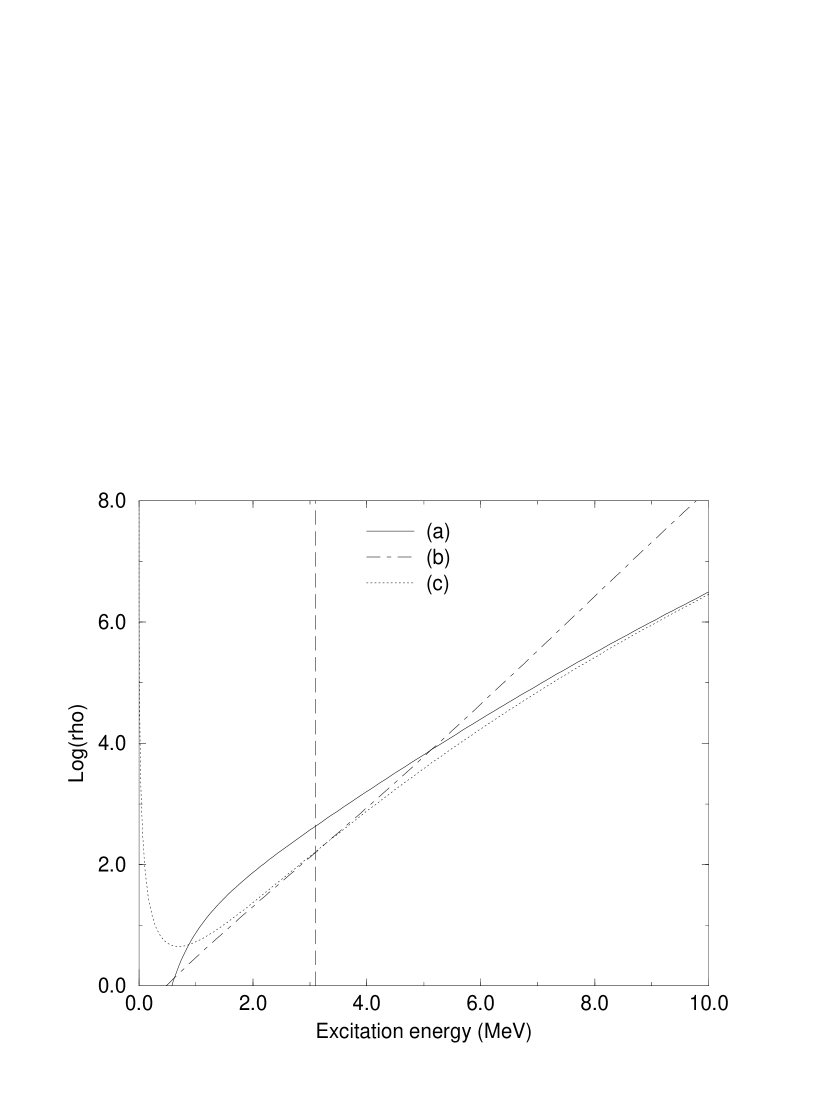
FIG. 1.: Level density for ${{}^{32}}S$; (a) modified saddle point, (b) corresponds to the fitted excitation energy as in fig. 4 and (c) usual saddle point. The vertical dashed line gives the position of 1st excitation level

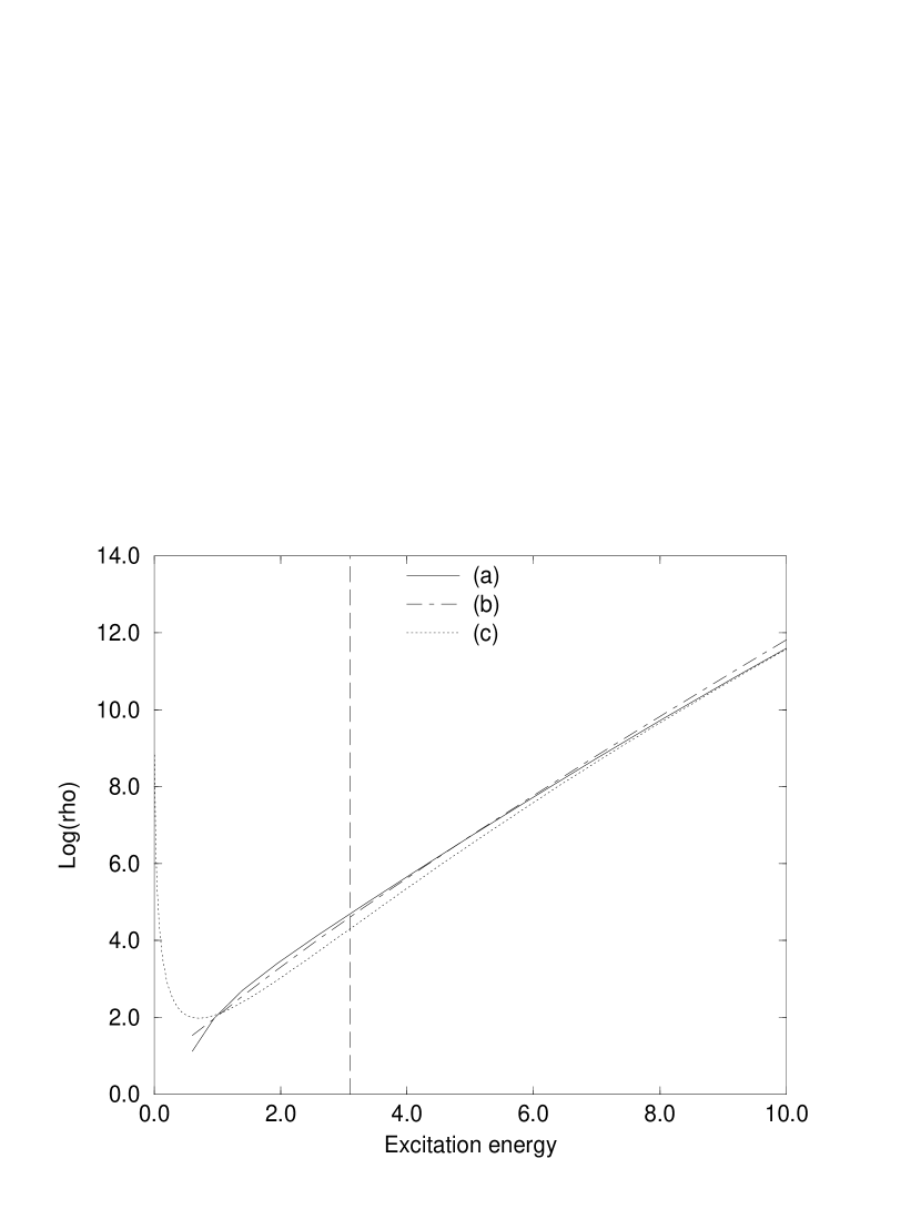
FIG. 2.: Level density for ${{}^{88}}Sr$; (a) modified saddle point, (b) corresponds to the fitted excitation energy as in fig. 4 and (c) usual saddle point. The vertical dashed line gives the position of 1st excitation level

FIG. 3.: Level density for ${{}^{208}}Pb$; (a) modified saddle point, (b) corresponds to the fitted excitation energy as in fig. 4 and (c) usual saddle point. The vertical dashed line gives the position of 1st excitation level

FIG. 4.: Excitation energy for ${{}^{32}}S$; (a) actual excitation energy nd (b) corresponds to the fitted form eq.(14) with $E_{0}$=5.62 and $\tau_{0}$=0.11

FIG. 5.: Excitation energy for ${{}^{88}}Sr$; (a) actual excitation energy nd (b) corresponds to the fitted form eq.(14) with $E_{0}$=15.71 and $\tau_{0}$=0.14

FIG. 6.: Excitation energy for ${{}^{208}}Pb$; (a) actual excitation energy nd (b) corresponds to the fitted form eq.(14) with $E_{0}$=40.0 and $\tau_{0}$=0.20

REFERENCES

- [1] T. Rausher, F.-K. Theielemann and K.-L. Kratz, Phys. Rev. C56, 1613 (1997).
- [2] N, Rosenweig, Phys. Rev. 105, 950 (1957); 108, 817 (1957).
- [3] A.G. Cameron, Can. J. Phys. 36, 1040 (1958).
- [4] A. Gilbert and A.G. Cameron, 43, 1446 (1965).
- [5] D. J. Dean, S. E. Kroonin, K. -H. Langnake, P. B. Radha and Y. Alhassid, Phys. Rev. Lett. 74, 2909 (1995).
- [6] V. Paar and R. Pezer, Phys. Rev. C55, R1637 (1997).
- [7] M.K. Grossjean and H. Feldmeier, Nucl. Phys. A444, 113 (1985).
- [8] J. R. Huizenga and L. G. Moretto, Ann. Rev. Nucl. Sc. 22, 427 (1972).
- [9] A. Bohr and B. R. Mottelson, Nuclear Structure Vol. II, World Scientific, (1998).