Coulomb displacement energies, energy differences and neutron skins.

Abstract

A Fock space representation of the monopole part of the Coulomb potential is presented. Quantum effects show through a small orbital term in $l(l+1)$. Once it is averaged out, the classical electrostatic energy emerges as an essentially exact expression, which makes it possible to eliminate the Nolen-Schiffer anomaly, and to estimate neutron skins and the evolution of radii along yrast states of mirror nuclei. The energy differences of the latter are quantitatively reproduced by the monopole term and a schematic multipole one.

PACS numbers: 21.10.Sf, 21.10.Ft, 21.10.Gv, 21.60.Cs, 27.40.+z

The electrostatic energy of a sphere of radius $R$ and charge $Ze$ is easily calculated to be $E_{Cs}=3e^{2}Z^{2}/5R$ ($E_{Cs}$ stands for “simple Coulomb energy”). It is under this guise that the Coulomb field enters the Bethe-Weizäcker mass formula, and becomes a basic quantity in nuclear structure. Direct evidence of entirely Coulomb effects has long been available from displacement energies between mirror (or in general, analog) ground states (CDE) [1, 2], and more recently from differences in yrast excitation energies in mirror $pf$-shell nuclei (CED) [3, 4, 5, 6, 7].

The CDE range from few to tens of MeV. They should be given mainly by $E_{Cs}$, but are underestimated by mean-field calculations: the Nolen-Schiffer (NS) anomaly [2], still an open problem.

The CED are very small (of the order of 10-100 keV). They have been semiquantitatively explained by shell model calculations using Coulomb matrix elements but there is some room for improvement.

The present letter intends to give a unified microscopic description of CDE and CED, by separating the Coulomb field into monopole and multipole components $V_{C}=e^{2}(M\omega/\hbar)^{1/2}/r=V_{Cm}+V_{CM}$ following ref. [8](DZ). The monopole $V_{Cm}$ contains all terms quadratic in scalar products of Fermion operators $a_{i}^{\dagger}\cdot a_{j}$. Its diagonal part involves only proton number operators, and should be responsible for $E_{Cs}$, and hence for the observed CDE. The non diagonal part will not be considered here: it leads to isospin mixing, but energetically its effect is small. The multipole $V_{CM}$ contains all non-monopole matrix elements and accounts for much of the CED.

As an introduction we examine the origin of the NS anomaly, by calculating $E_{Cs}$ with proton radii of the form

$$R_{\pi}=r_{0}\,A^{1/3}\left(1-\upsilon(\frac{t}{A})^{2}-\zeta\frac{t}{A^{4/3}}\right)e^{(1.75/A)}+{\cal D}.$$ (1)

($A=N+Z$, $t=N-Z$, $\pi,\,\nu\equiv$ protons, neutrons.)

Isospin conservation is assumed, which implies that $R_{\nu}$ is the same as $R_{\pi}$ for the mirror nucleus, obtained by interchanging $N$ and $Z$. Therefore, in Eq. (1), for $N>Z$, $\upsilon>0$ represents a uniform contraction of the two fluids, while $\zeta>0$ represents a $\pi$-contraction and a $\nu$-dilation. Hence, a (fractional) neutron skin can be defined as

$$\Delta(\zeta)=\frac{R_{\nu}-R_{\pi}}{r_{0}\,A^{1/3}\,e^{1.75/A}}=\frac{2|t|\zeta}{A^{4/3}},\quad N>Z.$$ (2)

The exponential factor takes care of the increase in $R_{\pi}$ observed in the light nuclei.

${\cal D}$ is a phenomenological term that accounts for shell and deformation effects. It is a sum of two quartic forms $\lambda S_{\pi}S_{\nu}+\mu Q_{\pi}Q_{\nu}$ that vanish at the spin-orbit (or EI: extruder-intruder) closures at $N$ or $Z=6,\,14,\,28,\,50,\,82,\,126$. Defining $D_{\pi}=(p_{\pi}+1)(p_{\pi}+2)+2$, the degeneracy of the EI_π shell (e. g., $p_{\pi}=3$ for $Z=28$ to 50), $D_{r\pi}=p_{\pi}(p_{\pi}+1)$, the degeneracy of the non-intruder subshells; the factors are $S_{\pi}=z(D_{\pi}-z)/D_{\pi}^{2}$ and $Q_{\pi}=z(D_{r\pi}-z)/D_{\pi}^{2}$ ($z$= number of valence protons). The parametrization is a variant of the ones in [9, 10].

Fits to $R_{\pi}=\sqrt{5\langle r_{\pi}^{2}\rangle/3}$—where $\langle r_{\pi}^{2}\rangle$ is the measured mean square radius—for 634 nuclei (with $N\geq Z$ except two cases!) yield ($r_{0}$ and rmsd in fm)

$r_{0}$=1.236   $\upsilon$=0.00  $\zeta$=0.94  $\lambda$=6.2   $\mu$=14.6   rmsd=0.018:

A good fit with a Huge Skin (HS hereafter).

$r_{0}$=1.220   $\upsilon$=0.61  $\zeta$=0.00  $\lambda$=5.7   $\mu$=27.0   rmsd=0.012:

A much better fit with Zero Skin (ZS hereafter).

$r_{0}$=1.226   $\upsilon$=0.45  $\zeta$=0.29  $\lambda$=5.7   $\mu$=24.0   rmsd=0.011:

An even better fit with a Minute Skin (MS hereafter).

Adding an exchange term to $E_{Cs}$, replacing $Z^{2}$ by $Z(Z-1)$ (conceptually better, as $V_{C}$ is two-body), the main contribution to the monopole energy takes the form

$$E_{Cm}=\frac{d\,Z(Z-1)(1-c\,Z^{-h})}{\rho},\quad d=\frac{3e^{2}}{5r_{0}}=\frac{0.864}{r_{0}},$$ (3)

$d$ in MeV and $\rho=(R_{\pi}-{\cal D})/{r_{0}}$: The $\cal D$ correction can be left out for simplicity as it does not affect what follows; the high quality fits become average ones (rmsd trebled), but still sufficient for our purpose. For the exchange term the usual choice is $h=2/3$, while $c$ varies appreciably [2]. Here we set $h=1$ (explained in and after Eq. (6)). The overall factor $d$ is fixed. Nevertheless, it will be allowed to vary, under the name $d_{f}$, together with $c$, in a fit to the 183 available CDE from reference [11]. The $\chi^{2}$ values are calculated by adding 200 keV to the experimental errors, to account for uncertainties in the calculations. Obviously, consistency between $R_{\pi}$ and $E_{Cm}$ demands $d_{f}=d$. The three fits to $R_{\pi}$ lead to:

$d$=0.699  $d_{f}$=0.77  $c=-0.5$  $\upsilon$=0.00  $\zeta$=0.94 $\chi^{2}$=0.91:

HS leads to a large overestimate of $d$. In other words: keeping the correct $d$ leads to a large underestimate of the CDE: the NS anomaly [2, 12], unresolved to this day (see however [13]).

$d$=0.708  $d_{f}$=0.69  $\,c$= 1.3  $\upsilon$=0.61  $\zeta$=0.00 $\chi^{2}$=1.46:

ZS leads to a small underestimate of $d$.

$d$=0.705  $d_{f}$=0.71  $\;c$= 0.9  $\,\upsilon$=0.45  $\zeta$=0.29 $\chi^{2}$=1.20:

MS leads to $d_{f}\approx d$. The NS anomaly disappears. Clearly, $\zeta\lessapprox 0.3$ is a good guess in Eq. (2).

The NS anomaly occurs because mean field calculations that yield good $R_{\pi}$ systematically overestimate $R_{\nu}$: Ref.[14] contains a nice illustration of the problem. It is ironical to note that a small neutron skin was recognized as a possible solution of the anomaly—but rejected—by Nolen and Schiffer [2]. Many reasons explain why this rejection held for so long. We retain only two: neglect of the $\upsilon(t/A)^{2}$ term in Eq. (1), and lack of confidence in the validity of $E_{Cm}$. As we show next, $E_{Cm}$ in Eq. (3) must be trusted, as it is basically an exact form of $V_{Cm}$.

By definition, the diagonal monopole part of $V_{C}$ is ($[J]=2J+1$):

$$V_{Cm}=\sum_{i\leq k}\frac{z_{i}(z_{k}-\delta_{ik})}{1+\delta_{ik}}V_{ik},\quad V_{ik}=\frac{\sum_{J}V_{Cikik}^{J}[J]}{\sum_{J}[J]}.$$ (4)

The label $k\equiv plj$ stands for the quantum numbers specifying a given harmonic oscillator (ho) orbit ($p$ is the principal quantum number). Restricting the sum to the first $\kappa$ major shells containing $\tau$ orbits, $V_{Cm}$ is brought to a sum of factorable terms by diagonalizing the matrix $\frac{1}{2}\{V_{ik}\}$ through the unitary transformation $\cal U$:

$$V_{Cm}=e^{2}\sqrt{\frac{M\omega}{\hbar}}\sum_{n}\left[{\cal E}_{n}\left(\sum_{k}z_{k}{\cal U}_{kn}\right)^{2}-{\cal C}\right],$$ (5)

where ${\cal C}=\sum_{n}z_{n}\,V_{nn}/2$ is the one-body counterterm in Eq. (4) left out of the diagonalization. By rescaling ${\cal E}_{n}=\tau E_{n}$, ${\cal U}_{kn}=(\tau)^{-1/2}U_{kn}$, the results become independent of $\tau$. To fix ideas choose $\kappa=8$, i. e., $\tau=36$. We expect to extract something close to the $Z^{2}$ operator, in which case only the highest eigenvalue ($E_{36}$) should be non vanishing, with $U_{k\,36}=1$. The diagonalization produces indeed an $E_{36}=0.192$ that is 30 times larger than the next and over 100 times larger than the second next. (Increasing the number of shells would only increase the number of negligible terms: Eq (5) is an exact representation in Fock space.) Fig. 1 shows that ($U_{k}\equiv U_{k\,36}$ ) is very well approximated by the form $U_{p}-0.01\,L^{2}$,

FIG. 1.: Dominant factor in the DZ decomposition of $V_{Cm}$

where $U_{p}=\sum_{j}(2j+1)U_{k}$ is the average of $U_{k}$ over $j$-values, and $L^{2}=l(l+1)-p(p+3)/2$ is an $l(l+1)$ term referred to its centroid. This result is still almost exact. The presence of $L^{2}$ is interesting, but here we average it out, to transform the operator $\sum_{p}z_{p}\,U_{p}$ into a c-number by taking expectation values in Eq. (5) over ho closed shells. Introducing $b=(\hbar/M\omega)^{1/2}$, we find

$$\langle V_{Cm}\rangle \approx \frac{e^{2}}{b}\left[E_{36}\langle\sum_{p}z_{p}U_{p}\rangle^{2}-\langle{\cal C}\rangle\right]$$ (6)

$$\approx \frac{e^{2}}{b}\left[E_{36}\left(\sum_{p}(p+1)(p+2)U_{p}\right)^{2}-\langle{\cal C}\rangle\right]$$ (7)

$$\approx \frac{e^{2}}{b}0.445\,(Z(Z-1))^{(1-1/12)}(1-0.96/Z).$$ (8)

The last line is a numerical fit to the previous one. $\langle\sum_{p}z_{p}U_{p}\rangle\approx 1.522Z^{1-1/12}(1-0.48/Z)$, so $0.445=0.192\times(1.522)^{2}$). In the exchange term: $Z^{-1}$ is better than $Z^{-2/3}$; 0.96 is close to $c$ in ZS and MS CDE fits. The apparently awkward 1-1/12 exponent comes out of the fit It will be seen to be natural once we extract $b$ from $\hbar\omega_{\pi}$ calculated as in [1, Eq. (2-157)], but treating separately neutrons and protons:

$$\hbar\omega_{\pi}=\frac{35.59(2Z)^{1/3}}{\langle r_{\pi}^{2}\rangle}\,\Longrightarrow\,\frac{e^{2}}{b}\,0.445=\frac{0.860Z^{1/6}}{r_{0}\,\rho},$$ (9)

where we have used $\langle r_{\pi}^{2}\rangle=3r_{0}^{2}\rho^{2}/5$ to bring Eq. (6) to the form of Eq. (3). The factor in $Z^{1/6}=(Z^{2})^{1/12}\approx(Z(Z-1))^{1/12}$ in $(\hbar\omega)^{1/2}$ conveniently corrects the “awkward exponent” and both equations become identical to within a 0.5% discrepancy in the $d$ coefficient: $0.860/r_{0}$ in Eq. (6) vs. $0.864/r_{0}$ in Eq. (3). Therefore, $E_{Cm}$ is essentially exact to within the averaging of $L^{2}$. A full treatment of this term is of obvious interest.

Let us turn to the CED in the $pf$ shell. They are differences in expectation values of $V_{C}$ for excitation energies; CED${}_{J}=E_{C}^{x}(Z,N,J)-E_{C}^{x}(N,Z,J)$ ($Z>N$). The wavefunctions are obtained through standard shell model calculations [15, 5, 6, 7] (they depend very little on the interaction: KB3, KB3G or FPD6). First we separate monopole and multipole pieces:

$${\rm CED}_{J}=\Delta\langle V_{Cm}\rangle_{J}+\Delta\langle V_{CM}\rangle_{J}$$ (10)

$\langle V_{Cm}\rangle_{J}$ is proportional to the difference of (inverse) radii between a $J$ yrast and the ground state: $R_{J}^{-1}-R_{0}^{-1}\approx(R_{J}-R_{0})/R_{0}^{2})$. Since $R_{J}$ is very nearly the same for both members of the mirror pair (remember: the neutron skin is small), it will be proportional to the average neutron plus proton occupancies for the individual orbits, which we denote by $\langle m_{k}\rangle_{J}/2$, with $m_{k}=z_{k}+n_{k}$ ($n_{k}$ is the number of neutrons). Now: to good approximation, the $R_{0}^{2}$ denominator is a constant over the region of interest ($A=47$-51) , furthermore, it is reasonable to assume that radii of the $pf$ orbits depend only on $l$, and, finally, the $p_{1/2}$ occupancy is always negligible. Therefore, $\langle V_{Cm}\rangle_{J}$ can be taken to depend only on $\langle m_{p_{3/2}}\rangle_{J}/2$.

The multipole contribution $\Delta\langle V_{CM}\rangle_{J}$ is given by the expectation values of the effective Coulomb potential in the $pf$ shell. Then

$${\rm CED}_{J}=a_{m}\langle m_{p_{3/2}}\rangle_{J}+\Delta\langle V_{Cpf}^{eff}\rangle_{J}$$ (11)

The value of $a_{m}$ can be estimated by noting that the single particle $p_{3/2}$ state in ⁴¹Sc is 200 keV below its analogue in ⁴¹Ca. This number comes from two effects: a larger radius that depresses the $p_{3/2}$ orbit, and the single particle $L^{2}$ term in Fig. 1 that depresses the $f_{7/2}$ ground state orbit. The latter effect is readily found to be $\approx$ 150 keV by expanding $(\sum_{k}U_{p}+.01L^{2})^{2}$ around the $A=40$ closed shell and using the numbers in, and after Eq. (6). Then, $a_{m}\approx(.200+.150)/2=0.175$ MeV. Note that the single particle contribution in $L^{2}$ is proportional to the difference of proton and neutron occupancies. It is important in $A=41$, but typically ten times smaller than the radial effect in $A=$47-51, so we have neglected it.

The available information on $\Delta\langle V_{Cpf}^{eff}\rangle_{J}$ involves only the $f_{7/2}$ matrix elements extracted from the ⁴²Ti-⁴²Ca pair, which yields ($7\equiv f_{7/2}$) $V_{CM\,7777}^{J}\equiv V_{Cf_{7/2}}^{eff}=$ (86.9, 116.9, 10.9, -59.1) keV, for $J$= 0, 2, 4, 6 respectively, to be compared with the ho values $V_{Cf_{7/2}}^{ho}$= (81.6, 24.6, -6.4, -11.4) keV. Since we are dealing with $V_{CM}$, the centroids $V_{77}$ (Eq. (4)) have been removed. They are very close (304 keV for $A$=42, 308 keV for ho) because $E_{Cm}$ depends on conserved quantities that cannot be renormalized. The multipole matrix elements are very different, and the data unequivocally prefer the $A=42$ set [5, 6]. The strategy adopted in these references was to use a $V_{Cpf}^{eff}$ with $V_{Cf_{7/2}}^{eff}$, keeping $V_{Cpf}^{ho}$ for the other matrix elements, which turned out to be almost irrelevant: the $V_{Cf_{7/2}}^{eff}$ set by itself accounts for the full $V_{Cpf}^{eff}$ chosen in this way. The results alternated between agreement and distorsion of the observed patterns.

As there is no justification in accepting an enormous renormalization for the $f_{7/2}$ orbits and leave the rest of the interaction unchanged, we shall attempt a more general treatment, by exploring the possibility of writing an effective interaction solely in terms of $V_{Cf_{7/2}}^{eff}$—properly renormalized to give a plausible account of the full $V_{Cpf}^{eff}$. First we check that the program can be enacted for the ho set. We try

$$\Delta\langle V_{Cpf}^{ho}\rangle_{J}=b\,\Delta\langle V_{Cf_{7/2}}^{ho}\rangle_{J}+a\,\langle m_{p_{3/2}}\rangle_{J}:$$ (12)

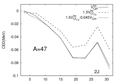
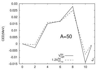
FIG. 2.: Calculated CED normalizations

Eq. (12) is only a numerical recipe, but it works well, as seen in Fig. 2, representative of the quality of the adjustment in the four cases (parameters in Tab I). Next, assume that the prescription applies to the renormalized case and try to invent an effective interaction consistent with the data and respecting the condition that the $a_{m}$ parameter in Eq. (11) be a constant that should be determined carefully: There is no room for invention here.

TABLE I.: Adopted parameters in Eq. (12) and Eq. (13)

$A$	$b$	$a$		$b_{M}$	$a_{M}$	$a_{m}$
47	1.5	-0.045		0.75	-0.080	0.150
49	1.5	0.000		0.75	0.000	0.150
50	1.2	0.000		0.60	0.000	0.150
51	1.6	-0.030		0.80	-0.054	0.150

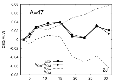
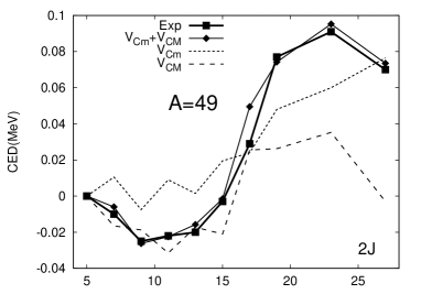
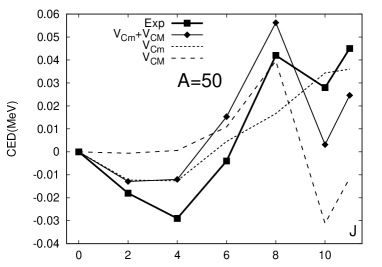
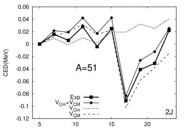
FIG. 3.: Experimental [4, 5, 6, 7] and calculated CED for the pairs ⁴⁷Cr-⁴⁷V, ⁴⁹Mn-⁴⁹Cr, ⁵⁰Fe-⁵⁰Cr, and ⁵¹Fe-⁵¹Mn.

Let us write

$$\text{CED}_{J} \equiv V_{Cm}+V_{CM}$$ (13)

$$= a_{m}\langle m_{p_{3/2}}\rangle_{J}+b_{M}\,\Delta\langle V_{Cf_{7/2}}^{eff}\rangle_{J}+a_{M}\langle m_{p_{3/2}}\rangle_{J}$$ (14)

For $A\approx 50$, $a_{m}$—estimated at $A=41$—must be reduced by a factor $(41/50)^{2/3}\approx 0.88$ to account for the $R_{0}^{2}$ denominator (after Eq. (11)). Therefore, we set $a_{m}=0.15$. Now choose $b_{M}=b/2$, $a_{M}=1.8\,a$. Eq. (13) with these parameters (Tab I) yields CED that in Fig. 3 are seen too agree well, even very well, with experiment. The mild exception is $A=50$, discussed in detail in Ref. [7], which contains a heuristic introduction to our CED results .

The monopole $V_{Cm}$ and multipole $V_{CM}$ contributions, shown separately in Fig.3, indicate that the latter reproduces only roughly the experimental patterns: The addition of $V_{Cm}$ is indispensable to bring quantitative agreement. It is especially worth noting that the strong signature effect in the $A=49$ band is erased in the CED by the out-of-phase $V_{Cm}$ and $V_{CM}$. Conversely, the signature staggering is enhanced in $A=51$.

The monopole contribution provides valuable information about the evolution of yrast radii. As a consequence, the use—and even the validity—of the schematic multipole term (the “invention”) must be assessed by the focus it brings to the monopole one, which must be present in a form very close to that in Eq. (11).

To conclude: once the NS anomaly is resolved, the Coulomb field fulfills the—long held—hope of providing information about radii not directly measured. The $L^{2}$ terms offers intriguing prospects. A complete analysis of $V_{Cm}$, including non-diagonal contributions, is in order to estimate isospin impurities. The renormalization of $V_{CM}$ remains an open problem.

This work owes much to a stay of AZ at the UAM, made possible by a scholarship of the BBVA foundation.

REFERENCES

- [1] A. Bohr and B. Mottelson, Nuclear Structure vol I (Benjamin, Reading, 1964).
- [2] J. A. Nolen and J. P. Schiffer, Ann. Rev. Nuc. Sci. 19, 471 (1969)
- [3] J.A. Sheikh, P. Van Isacker, D.D. Warner and J.A.Cameron, Phys. Lett. B 252, 314 (1990).
- [4] C. O’Leary et al., Phys. Rev. Lett. 79, 4349 (1997).
- [5] M.A. Bentley et al., Phys. Lett. B 437, 243 (1998).
- [6] M.A. Bentley et al., Phys. Rev. C 62, 051303(R) (2000).
- [7] S. M. Lenzi et al., submitted to PRL.
- [8] M. Dufour and A. P. Zuker, Phys. Rev. C 54, 1641 (1996).
- [9] J. Duflo, Nucl. Phys. A576, 29 (1994).
- [10] J. Duflo and A. P. Zuker, Phys. Rev. C 59, R2347 (1999).
- [11] G. Audi and A.H. Wapstra, Nucl. Phys. A595, 409 (1995).
- [12] N. Auerbach, Phys. Rep. 98, 273 (1983).
- [13] A. Bulgac and R. Shaginyan, Phys. Lett. B 469, 1 (1999), S. A. Fayans and D. Sawischa, nucl-th/0009034.
- [14] J. Bartel, M. B. Johnson, M. K. Singham and W. Stocker, Phys. Lett. B 296, 5 (1992).
- [15] E. Caurier, ANTOINE code, Strasbourg (1989-2001).