New results for $2\nu\beta\beta$ decay with large particle-particle two body proton-neutron interaction

Abstract

A model many-body Hamiltonian describing an heterogenous system of paired protons and paired neutrons and interacting among themselves through monopole particle-hole and monopole particle-particle interactions is used to study the double beta decay of Fermi type. The states are described by time dependent approaches choosing as trial functions coherent states of the symmetry groups underlying the model Hamiltonian. One formalism, VP1, is fully equivalent with the standard pnQRPA and therefore fails at a critical value of the particle-particle interaction strength while another one, VP2, corresponds to a two step BCS treatment, i.e. the proton quasiparticles are paired with the neutron quasiparticles. In this way a harmonic description for the double beta transition amplitude is provided for any strength of the particle-particle interaction. The approximation quality is judged by comparing the actual results with the exact result as well as with those corresponding to various truncations of the boson expanded Hamiltonian and transition operator. Finally it is shown that the dynamic ground states provided by VP1 and VP2 are reasonable well approximated by solutions of a variational principle. This remark constitutes a step forward finding an approach where the RPA ground state is a solution of a variational principle equation.

I Introduction

One of the most exciting subject of the modern nuclear physics is the double beta decay. The reason is that from this field one expects an answer to the question of whether neutrino is a Majorana or a Dirac particle. The process may take place through one of two channels, 0$\nu\beta\beta$ and $2\nu\beta\beta$. The answer to the above mentioned question might come from the discovery of the first process which if it exists requires that the neutrino is a Majorana particle and which should be a rare one [1, 2, 3, 4, 5, 6]. In order to make predictions of the neutrino mass and the right handedness of its electroweak interactions one should use reliable nuclear matrix elements. However there is no stringent test for these matrix elements. Fortunately for the double beta decay with two anti-neutrinos in the final state $2\nu\beta\beta$, one uses similar nuclear matrix elements and moreover for this process plenty of data exist. Therefore the idea of using for the neutrino-less double beta decay the same many-body approach and the same NN force which describe realistically the two neutrino double beta decay, was adopted by most of the groups involved in such studies. Actually this is the reason why so many theoreticians focused their attention in explaining the features of the experimentally measured $2\nu\beta\beta$ process [7, 8, 9, 10, 11, 12, 13]. The formalism which predicts decay rates closest to the experimental data is the proton-neutron quasiparticle random phase approximation (pnQRPA) which includes the particle-particle ($pp$) two body interaction. Without this interaction the predicted transition amplitude is too large as compared to the existent data. Including the $pp$ interaction and considering its strength, $g_{pp}$, as a free parameter one obtains the following behavior for the transition amplitude. For a large interval of $g_{pp}$, starting from zero, there exists a plateau followed by a quick decrease. The amplitude vanishes at a certain $g_{pp}$ and shortly after this point one reaches, with increasing $g_{pp}$, the critical value where the pnQRPA breaks down. On the decreasing part of the $2\nu\beta\beta$ transition amplitude as a function of $g_{pp}$ one finds agreement with experiment. The drawback of this description is that in this area of $g_{pp}$, the pnQRPA is not a good description and therefore the results are not stable to adding higher RPA correlations. Many attempts have been made to stabilize the ground state in this region of the particle-particle interaction. The new methods tried either to keep the pnQRPA boson picture but include higher correlations through boson expansion [14, 15, 16, 17, 18, 19] techniques or via self-consistent procedures [20], or to re-normalize the pnQRPA phonon [21, 22, 23, 24]. These methods improved the description of the data[25] although they have also drawbacks and lack sometimes of consistency [24, 26, 28].

In a previous paper [26] we advanced the idea that the ground state may be stabilized by introducing the particle-particle interaction first in the mean field and then to the pnQRPA process. A way to do that is even possible at the level of independent quasiparticle representation. Indeed, we noticed in a schematic single j model [29] that one term of the two body quasiparticle interaction is a quasiparticle proton-neutron pairing interaction and its strength is negative. Therefore one could define a Cooper pair out of one proton quasiparticle and one neutron quasiparticle. This was worked out through a time dependent variational principle. We chose alternatively four distinct trial functions. Two of these define different RPA approaches. One is identical to the standard pnQRPA and works for small strengths of the particle-particle interaction, namely before the critical point, whereas the other one provides a harmonic picture beyond the critical value of the interaction strength, i.e. in the region where the standard pnQRPA does not work at all. Moreover in this region a boson expansion procedure might be defined and through diagonalization the exact result can be recovered.

In the present paper we continue the study started in the previous paper, by focusing on the following new features. Here we calculate the double beta decay transition amplitude by using the description in the interval of the particle-particle interaction forbidden for the pnQRPA approach. We hope that by matching the approaches in the two complementary intervals one could provide a unified description of the process for small as well for large strengths of the particle-particle interaction. When one uses the boson expansion for the model Hamiltonian one aims at testing the convergence properties by comparing the corresponding results with the exact ones. One should mention that this is possible only for a single j model Hamiltonian involving a monopole two body interactions. Formulating it for the double beta decay Fermi transition the boson expansion of the transition operator emitted in ref.[14] is a Schwinger type boson expansion since it uses two different bosons in order to satisfy the condition of mapping two algebras. This is a good test for the boson representation which was previously used. Another aspect which is treated here refers to the structure of the vacuum states provided by the standard pnQRPA and the approach which works beyond the critical particle-particle interaction strength. We want to check whether these two vacua might be described in a reasonable approximative fashion by static ground states yielded by a variational principle with a suitable trial function.

This project is achieved according to the following plan. In Section 2, a brief review of the results obtained in the previous paper is given. These results are used here for a self-consistent presentation. In Section 3, we compare the results for double beta decay transition amplitude obtained in the two intervals of the particle-particle interaction, i.e. before and after its critical value, with different methods. In Section 4 the Holstein-Primakoff boson representation is used for the model Hamiltonian. By diagonalizing the full Hamiltonian, the first order approach and the results for the limit $\Omega\rightarrow\infty$ and by comparing the results with the exact ones and those obtained within the harmonic picture, one could judge the convergence quality of the expansion used. The Schwinger type boson representation is here also applied. The possible contribution of pairing vibrational states to the enhancement of the decay rate is discussed. The decay to the double phonon pairing vibration is explicitly analyzed. In Section 5 we study a possible relationship between the vacuum states of the standard pnQRPA, the second order BCS approach, and the static ground state provided by classical variational equations obtained with two different trial functions. Final conclusions are drawn in Section 6.

II Brief review of some previous results

Since the present paper is continuing the study we started in previous publications we give here a brief summary of the main ingredients used there [26]. In this way we fix the notation and the conventions. Also the general frame of our present results will be better emphasized. The object of our study is a system of protons and neutrons moving in a spherical shell model mean field, interacting among themselves through pairing, particle-hole and particle-particle monopole two body interaction. The associated Hamiltonian reads:

$$H = \epsilon_{p}\sum_{m}c^{\dagger}_{pm}c_{pm}+\epsilon_{n}\sum_{m}c^{\dagger}_{nm}c_{nm}$$ (1)

$$- \frac{G_{p}}{2}P^{\dagger}_{p}P_{p}-\frac{G_{n}}{2}P^{\dagger}_{n}P_{n}$$ (2)

$$+ 2\chi\beta^{-}\beta^{+}-2\chi_{1}P^{-}P^{+}~{}~{},$$ (3)

where the following notations have been used:

$$P^{\dagger}_{p} = \sum_{m}c^{\dagger}_{\tau m}c^{\dagger}_{\widetilde{\tau m}},\tau=p,n,$$ (4)

$$\beta^{-} = \sum_{m}c^{{\dagger}}_{pm}c_{nm};\beta^{+}=(\beta^{-})^{+},$$ (5)

$$P^{-} = \sum_{m}c^{{\dagger}}_{pm}\widetilde{c}^{{\dagger}}_{nm};P^{+}=(P^{-})^{+}.$$ (6)

The standard notations for the creation and annihilation operators are used. For the sake of simplicity we consider here the case of a single j shell. The extension to the multi-shell picture is straightforward. However for the purposes of the present study the multi-shell calculations are not necessary. The shell j is self-understood in our notations. To specify the isospin of the particle occupying the shell we use the indices p for proton and n for neutrons. The time reversed state is denoted by $|\widetilde{\tau m}\rangle=(-1)^{j-m}|\tau,-m\rangle$. Performing the Bogoliubov-Valatin transformation, the model Hamiltonian is transformed in a many body quasiparticle operator which after ignoring the quasiparticle scattering terms and, for the sake of simplicity, equating the proton and neutron single particle energies, has the form:

$$H=\epsilon(\hat{N}_{p}+\hat{N}_{n})+\lambda_{1}A^{{\dagger}}_{pn}A_{pn}+\lambda_{2}(A^{{\dagger}}_{pn}A^{{\dagger}}_{pn}+A_{pn}A_{pn}),$$ (7)

where ${\hat{N}}_{p}$ and ${\hat{N}}_{n}$ are the proton and neutron quasiparticle number operators, respectively, while $A^{+}_{pn},A_{pn}$ stand for the proton-neutron pairing operators built up with the quasiparticle operators $a^{{\dagger}}_{pm},a^{{\dagger}}_{nm}$:

$$A^{{\dagger}}_{pn}=[a^{{\dagger}}_{p}a^{{\dagger}}_{n}]_{00},\;A_{pn}=(A^{{\dagger}}_{pn})^{{\dagger}}.$$ (8)

The coefficients $\epsilon,\lambda_{1},\lambda_{2}$ are functions of the parameters defining the Hamiltonian (2.1) as well as of the coefficients U, V determining the quasiparticle representation. The Hamiltonian (2.3) is a quadratic expression in the generators of the SU(2) algebra

$$\hat{S}_{0}=\frac{1}{2}[\hat{N}_{p}+\hat{N}_{n}-2\Omega],~{}~{}\hat{S}_{+}=\sqrt{2\Omega}A^{{\dagger}}_{pn},~{}~{}\hat{S}_{-}=\sqrt{2\Omega}A_{pn},~{}~{}\Omega=\frac{2j+1}{2}.$$ (9)

and therefore it is exactly solvable. This feature has the great advantage that one could test the many body approximations adopted in various formalisms. This virtue made it very attractive for many theoreticians who used it widely to advance some new hypothesis for treating the proton-neutron two body interaction [29, 30, 31].

One may argue that restricting the model space to a single j level one misses the effect of spin-orbit interaction. However from our earlier studies [32, 33], we now that the spin orbit coupling is important for the Gamow-Teller double beta transition, where most of the strength is carried by spin-flip configurations, but not for the Fermi transition which we are studying in the present paper.

If one assumes that the monopole two quasiparticle operators and their hermitian conjugate satisfy bosonic like commutation relations than a harmonic excitation operator might be defined. Therefore the Weyl algebra, defined by the operators $A^{\dagger},A,I$ (here $I$ denotes the unity operator), can be used to describe the eigenstates of H. When the terms with four quasiparticles in H are dominant and the quasiboson approximation is adopted, for the above mentioned commutators, one could diagonalize first the anharmonic part of H and then treat the term expressing the quasiparticle total number operator. Up to an additive constant, the anharmonic part of H (four quasiparticle terms) is a linear combination of the generators of the group $SU(1,1)$, i.e. ${A^{+}}^{2},A^{2},2+4A^{+}A$. Therefore this symmetry might be useful for describing the eigenstates of H.

The model Hamiltonian (2.1) was treated, in ref.[26], within a dependent variational principle formalism:

$$\delta\int^{t}_{0}\langle\psi|H-i\frac{\partial}{\partial t^{\prime}}|\psi\rangle dt^{\prime}=0.$$ (10)

by taking as trial functions the coherent states of the above mentioned symmetry groups. Since the coherent state for SU(2) and for the Weyl group are formally identical with the difference that in the first case the operators $A^{\dagger},A$ satisfy exact commutation relations, while in the later case they are considered as quasibosons, we complete our study with a fourth wave function which is similar to the SU(1,1) coherent state but the operators involved satisfy exact commutation relations. Concluding, the following trial functions have been alternatively considered for the variational state [26, 27]:

$$|\psi_{1}(z,z^{*})\rangle = exp\{zA^{{\dagger}}_{pn}-z^{*}A_{pn}\}|0\rangle_{q},~{}\left[A_{pn},A^{\dagger}_{pn}\right]=1,~{}~{}\rm{(VP1)}$$ (11)

$$|\psi_{2}(z,z^{*})\rangle = exp\{zA^{{\dagger}}_{pn}-z^{*}A_{pn}\}|0\rangle_{q},\left[A_{pn},A^{\dagger}_{pn}\right]=1-\frac{1}{2\Omega}({\hat{N}}_{p}+{\hat{N}}_{n}),~{}~{}\rm{(VP2)}$$ (12)

$$|\psi_{3}(z,z^{*})\rangle = \exp(z{A^{{\dagger}}_{pn}}^{2}-z^{*}{A_{pn}}^{2})|0\rangle_{q},~{}\left[A_{pn},A^{{\dagger}}_{pn}\right]=1,~{}~{}\rm{(VP3)}$$ (13)

$$|\psi_{4}(z,z^{*})\rangle = {\cal N}_{4}e^{z{A^{{\dagger}}_{pn}}^{2}}|0\rangle_{q},~{}[A_{pn},A^{\dagger}_{pn}]=1-\frac{1}{2\Omega}({\hat{N}}_{p}+{\hat{N}}_{n}),~{}~{}\rm{(VP4)}$$ (14)

In each case, $z$ is a complex function of time and $z^{*}$ denotes its complex conjugate. $|0\rangle_{q}$ is the quasiparticle vacuum state. The formalism corresponding to the trial function $|\Psi_{k}\rangle$ with the commutation relations specified above, will be hereafter called VPk. For each of the four cases we solved the static equations of motion and then found the harmonic mode describing small oscillations around the static ground state. Several properties such as the behavior of energies with respect to the strength of the particle-particle interaction, as the ground state correlations, as the single beta transition amplitude, as the Ikeda sum rule and also various quantization procedures of the classical equations of motion have been analyzed. For a better presentation the final results will be considered, as in ref.[26, 29], as function of the re-scaled strengths of particle-hole and particle-particle interactions:

$$\chi^{\prime}=2\Omega\chi,~{}~{}k^{\prime}=2\Omega\chi_{1}.$$ (15)

For example the energies of the first excited states in mother and daughter nuclei, predicted by VP1 and VP2, vary with $k^{\prime}$ as in Fig 1. while those given by VP3 and VP4 as shown in Fig 2.

Here we complete this analysis with some new properties of the proton-neutron interacting system.

III Double beta decay

The double beta decay with two anti-neutrinos in the final state is considered to take place by two consecutive single $\beta^{-}$ decays. The intermediate state reached after the first beta decay, consists of an odd-odd nucleus in a pn excited state, one electron and one anti-neutrino. If in the intermediate state, the total lepton energy is approximated by the sum of the electron mass and half of the Q-value of the double beta decay process ($\Delta E$), the inverse of the process half-life can be factorized as follows :

$$(T^{2\nu}_{1/2})^{-1}=F|M_{F}|^{2},$$ (16)

where F is a lepton phase integral while the second factor is determined by the states characterizing the nuclei involved in the process and has the expression:

$$M_{F}=\sum_{k,k^{\prime}}\frac{{{}_{m}}\langle 0^{+}|\beta^{+}|0^{+}_{k}\rangle_{m}{{}_{m}}\langle 0^{+}_{k}|0^{+}_{k^{\prime}}\rangle_{d}{{}_{d}}\langle 0^{+}_{k^{\prime}}|\beta^{\dagger}|0^{+}\rangle_{d}}{E_{k}+\Delta E},$$ (17)

where the transition operators is defined by eq (2.2). The initial and final states are the ground states of mother ($|0^{\dagger}\rangle_{m}$) and daughter ($|0^{\dagger}\rangle_{d}$) nuclei. These states are vacuum states for the pnQRPA phonon operators built on the top of the corresponding BCS states which are the static ground states. The matrix elements describing the first and the second legs of the process have been calculated in a previous publication based on the semi-classical approaches (see eqs. 6.25 and 6.32 from ref.[26]) VP1 and VP2. In both cases there is only one excited states and therefore the summation in eq. (3.2) can be omitted. The overlap matrix element involved in Eq. (3.2) is function of the forward (X) and backward (Y) amplitudes of the harmonic boson and has the expression:

$${{}_{m}}\langle 0^{+}_{1}|0^{+}_{1}\rangle_{d}=X_{m}X_{d}-Y_{m}Y_{d},$$ (18)

where the indices m and d specify that the corresponding states describe the mother and daughter nuclei, respectively. The energy denominator in Eq (3.2) is:

$$E_{1}=\omega_{m},$$ (19)

where $\omega_{m}$, is the energy of the harmonic mode in the mother nucleus. The results for the double beta transition amplitude obtained within the VP1 and VP2 approaches are plotted in Fig. 3 a) as function of the proton-neutron pairing strength k’. In the VP1 approach the energy shift $\Delta E$ is taken equal to 1 MeV. The same $\Delta E$ is considered for the first part of the k’ interval in Fig. 3 b). For the strength of the proton-neutron pairing $k^{\prime}\geq 1.3MeV$ this energy shift is corrected by half the difference between the static ground state energies in the mother and daughter nuclei. From there we see that the transition amplitude for small ($k^{\prime}<0.8$MeV) and large ($k^{\prime}>1.5$MeV) k’ is almost constant. Moreover there is a finite interval for $k^{\prime}$ where the amplitude is not defined. The justification for such a window can be seen in Fig 1. Indeed from the lower panel it is clear that the VP1 approach yields a transition amplitude which is not defined beyond $k^{\prime}=1.05$ since the harmonic mode in the daughter nucleus collapses. In the upper panel of Fig.1 it is shown that the SU(2) mode in the mother nucleus has a non-vanishing energy only for values of k’ larger than 1.2 for $\chi^{\prime}=0.$ and 1.3 for $\chi^{\prime}=0.5$.

IV Boson Expansion

For the VP2 formalism several classical canonical coordinates have been found. To each set of coordinates corresponds a specific quantization scheme. Through the quantization procedure, the classical energy function is transformed to an operatorial function of boson operators. In what follows we shall use two boson representations of the model Hamiltonian. In each case the corresponding eigenstates are used to evaluate, by means of eq. (3.2) , the transition amplitude for the double beta Fermi transition.

A Holstein Primakoff boson expansion

The Holstein-Primakoff boson mapping [34] corresponds to the following canonical complex coordinates:

$$C^{*}=\sqrt{2\Omega}V;~{}~{}C=\sqrt{2\Omega}V^{*},$$ (20)

Indeed in these coordinates the classical equations of motion are in the canonical form:

$$\{C^{*},C\}=i,~{}~{}\{C^{*},{\cal H}\}=\stackrel{{\scriptstyle\bullet}}{{C^{*}}},~{}~{}\{C,{\cal H}\}=\stackrel{{\scriptstyle\bullet}}{{C}}.$$ (21)

Through the quantization

$$(C_{1},C_{1}^{*};i\{,\})\rightarrow(B,B^{{\dagger}};[,]),$$ (22)

the classical SU(2) algebra, generated by the averages of the fermionic SU(2) algebra on the coherent state $|\Psi_{2}\rangle$, is mapped onto a boson SU(2) algebra. Multiplying the two applications one obtains a mapping of the fermionic algebra onto a boson SU(2) algebra. The result is conventionally called as the boson expansion of the initial fermionic generator operators. Since this boson expansion for the generators of the SU(2) algebra has been found first by Holstein and Primakoff we shall refer to it as to the HP boson expansion. By the mapping specified by eq.(4.3), any function of the complex coordinates $C^{*},C$ can be transformed into a function of the bosons $B^{\dagger},B$. In particular the classical energy ${\cal H}$, the average of H (2.1) on $|\Psi_{2}\rangle$, is transformed in the HP boson expansion of the model Hamiltonian:

$$H_{B}^{(HP)} = 2\epsilon B^{{\dagger}}B+\lambda_{1}(B^{{\dagger}}B-\frac{1}{2\Omega}{B^{+}}^{2}B^{2})$$ (23)

$$+ \lambda_{2}[{B^{+}}^{2}\sqrt{(1-\frac{\hat{N}+1}{2\Omega})(1-\frac{\hat{N}}{2\Omega})}+\sqrt{(1-\frac{\hat{N}+1}{2\Omega})(1-\frac{\hat{N}}{2\Omega})}B^{2}].$$ (24)

In the limit of $\Omega$ going to infinity the Hamiltonian $H^{(HP)}_{B}$ goes to:

$$\widetilde{H}_{B}^{(HP)}=(2\epsilon+\lambda_{1})B^{{\dagger}}B+\lambda_{2}({B^{{\dagger}}}^{2}+B^{2}).$$ (25)

We shall refer to $\widetilde{H}_{B}^{(HP)}$ as the Hamiltonian in the zeroth order boson expansion. The Hamiltonian in the first order boson expansion is:

$$H^{(1)}_{HP}=(2\epsilon+\lambda_{1})B^{{\dagger}}B+\lambda_{2}\frac{4\Omega-1}{4\Omega}({B^{{\dagger}}}^{2}+B^{2})-\frac{\lambda_{2}}{2\Omega}({B^{{\dagger}}}^{2}{\hat{N}}+{\hat{N}}B^{2})-\frac{\lambda_{1}}{2\Omega}{B^{{\dagger}}}^{2}B^{2}.$$ (26)

The transition operator linking the states described by the boson Hamiltonians (4.4), (4.5) and (4.6) has the expressions

$$\beta^{{\dagger}} = \sqrt{2\Omega}\left[U_{p}V_{n}\sqrt{1-\frac{B^{{\dagger}}B}{2\Omega}}B+V_{p}U_{n}B^{{\dagger}}\sqrt{1-\frac{B^{{\dagger}}B}{2\Omega}}\right],$$ (27)

$$\beta^{{\dagger}} = \sqrt{2\Omega}\left[U_{p}V_{n}B+V_{p}U_{n}B^{{\dagger}}\right],$$ (28)

$$\beta^{{\dagger}} = \sqrt{2\Omega}\left[U_{p}V_{n}(1-\frac{B^{{\dagger}}B}{4\Omega})B+V_{p}U_{n}B^{{\dagger}}(1-\frac{B^{{\dagger}}B}{4\Omega})\right],$$ (29)

respectively. The matrix elements involved in the transition amplitude can be easily calculated. To save space here we describe only the results for the first order expansion. Diagonalizing the matrix associated to the boson Hamiltonian $H^{(1)}_{HP}$, given in Appendix A, in the basis

$$|m\rangle=\frac{1}{\sqrt{m!}}{B^{{\dagger}}}^{m}|0\rangle_{b},$$ (30)

for the case of mother (m) and daughter nuclei (d), one obtains the eigenstates:

$$|0^{+}_{k}\rangle_{p}=\sum_{l}C^{(p)}_{k,l}|l\rangle,~{}~{}p=m,d,~{}~{}k=0,1,2,..$$ (31)

Here $|0\rangle_{b}$ denotes the vacuum state for the boson B. The corresponding eigenvalues will be denoted by $E^{(p)}_{k}$. The label $k=0$ corresponds to the ground state and to simplify notations we shall omit it. To be more suggestive sometimes the label ”0” is replaced by ”g”. The overlap of the states describing the mother and daughter nuclei have the form:

$${{}_{m}}\langle 0^{+}_{k}|0^{+}_{k^{\prime}}\rangle_{d}=\sum_{l}C^{(m)}_{k,l}C^{(d)}_{k^{\prime},l}.$$ (32)

The matrix elements of the transition operator can be easily calculated once one knows how to calculate the matrix elements corresponding to the basis states. These are given explicitly in Appendix A. The energy denominator in Eq. (2.2), corresponding to the boson expansion treatment, is defined as follows:

$$E_{k}=E^{(m)}_{k}-E^{(m)}_{g}.$$ (33)

The energy shift $\Delta E$ was taken equal to 1MeV for small values of the proton-neutron pairing strength k’ while for large k’, half of the difference between the static ground state energies of mother and daughter nuclei is added to this value. The double beta transition amplitude, calculated by using the eigenstates of $\widetilde{H}_{B}^{(HP)}$ is shown in the lower plot of Fig.3, lowest panel. Since the ground states of the mother and daughter nuclei contain many boson components the transition operator, although it is linear in bosons, may excite the ground states to a many boson state describing the intermediate odd-odd nucleus. Therefore for the intermediate states in Eq. (3.2) the complete set produced by the diagonalization procedure was considered. We found that the first excited state of the above mentioned complete set contributes the largest part to the double beta transition amplitude. The general trends shown in the upper and lower panel are similar to each other. While the left branches are identical, the second branch corresponding to the zeroth boson expanded Hamiltonian is much larger than that produced by the harmonic approximation defined by using the coherent state for the $SU(2)$ group, as variational state. This indicates that for these values of k’ the anharmonic effects prevail over the harmonic ones. While in the upper panel we notice an interval where the transition amplitude is not defined, the transition amplitude in the lower panel is vanishing in this interval. The reason is that the mixture of the higher boson states is large and different components have different phases and therefore their partial contributions cancel each other. The results for the double beta transition amplitude corresponding to the full HP boson expanded Hamiltonian are compared in Fig. 4 with those obtained with the first order boson expanded Hamiltonian . One remarks that sizable differences are noticed only for large values of k’. It is worth to mention that while in the lower panel of Fig.3 the window where the transition amplitude vanishes is for a finite range of k’, here this is reduced just to a point. As we showed in ref.[26] the HP boson expansion is defined in that interval of k’ where the standard pnQRPA does not work. However the final boson Hamiltonian can be diagonalized also for k’ belonging to the region where the standard pnQRPA properly works. In this region however the boson cannot be interpreted as describing small oscillations around a ”deformed” minimum but around the origin of the phase space. We would like to mention the fact that the results obtained with the eigenstates of the full HP Hamiltonian coincide with the exact result corresponding to the exact eigenstates of the fermionic quasiparticle Hamiltonian [26]. Comparing the results shown in Figs. 3 (first panel) and 4 one may say that in the first interval of k’ the pnQRPA works quite well, the corresponding results lie close to the exact ones. By contrast for large values of k’, the results corresponding to the harmonic approximation are quite different from the exact ones. The exact result indicate that a big effect is caused by anharmonicities.

B Schwinger boson expansion

In ref. [14]we proposed a boson expansion formalism for treating the Gamow-Teller double beta transition. The underlying idea was that the boson series associated to two quasiparticle proton neutron operators should be chosen in such a way that the mutual commutation relations for the fermionic operators are satisfied in each order of the approximation. This condition could not be satisfied if we restricted the space to the pnQRPA bosons. However, the condition is fulfilled if the space is extended by including also the quadrupole charge conserving QRPA bosons. Therefore the boson representation of the bifermionic proton-neutron operators contains two types of bosons and therefore we call it Schwinger like boson expansion. Schwinger [35] was the first who achieved a boson mapping of the SU(2) algebra by using two bosons. A weak point of boson expansions for many body operators is that there is no quantitative measure for the ”rest” when the infinite series is truncated. However, in the present case the evaluation of the ”rest” is possible since one knows the exact result. Therefore it is worth to formulate the boson expansion, used in ref.[14] for GT double beta transition, for the case of Fermi transition. In this case the charge conserving boson, which should be added to the proton-neutron QRPA boson in order to fulfill the condition of preserving the mutual commutation relations, is the pairing vibrational mode. This mode is a particle-particle like excitation and its amplitudes are related to the overlap of the function describing the given nucleus with a one associated to a system obtained by adding (or subtracting) a pair of protons or a pair of neutrons. It is worth to remark that the daughter nucleus involved in a Fermi double beta decay is a component of a double phonon vibrational state obtained by removing a pair of neutrons and adding a pair of protons. Since the daughter nucleus could be reached by transforming the mother nucleus in two different ways, the double beta decay and the double phonon excitation, one may expect that the anharmonic part of the boson expanded transition operator for single beta decay leg might excite two boson and three boson states in the intermediate odd-odd nucleus having one and two charge conserving phonon factors, respectively. The pairing vibrational modes are usually defined by the proton-proton and neutron-neutron pairing interactions. Therefore there are proton and neutron vibrational modes which are decoupled from each other. Within the QRPA approach there are two spurious states due to the conservation of both the number of protons and the number of neutrons. When the space of single particle states is restricted to a single shell there is no physical solution. In order to allow a non-vanishing energy, one needs at least an additional level where to promote a pair of particles. To keep simplicity we maintain the single j picture but consider the contribution of the proton-neutron particle-hole and particle-particle interactions to the equations of motion of the charge conserving operators. In this way, for example, the single j of the neutron system will play the role of the second level for the equations of motion of the proton-proton monopole operators. Therefore we keep, in the quasiparticle representations of the model Hamiltonian, the terms with four quasiparticle operators which contribute to the equations of motion of two quasiparticle monopole operators:

$$H_{q} = E^{\prime}_{p}\hat{N}_{p}+E^{\prime}_{n}\hat{N}_{n}$$ (37)

$$-\frac{G_{p}}{4}2\Omega\left[(U_{p}^{4}+V_{p}^{4})A^{\dagger}_{pp}A_{pp}-U_{p}^{2}V_{p}^{2}(A_{pp}^{\dagger^{2}}+A_{pp}^{2})+4U_{p}^{2}V_{p}^{2}B_{pp}^{\dagger}B_{pp}\right]$$

$$-\frac{G_{n}}{4}2\Omega\left[(U_{n}^{4}+V_{n}^{4})A^{\dagger}_{nn}A_{nn}-U_{n}^{2}V_{n}^{2}(A_{nn}^{\dagger^{2}}+A_{nn}^{2})+4U_{n}^{2}V_{n}^{2}B_{nn}^{\dagger}B_{nn}\right]$$

$$+\lambda_{1}A_{pn}^{\dagger}A_{pn}+\lambda_{2}\left[A_{pn}^{\dagger^{2}}+A_{pn}^{2}-B_{pn}^{\dagger^{2}}-B_{pn}^{2}\right],$$

where the following notations have been used:

$$E^{\prime}_{p} = E_{p}+\frac{G_{p}}{2}V_{p}^{4}+2(U_{p}^{2}-V_{p}^{2})(\chi U_{n}^{2}-\chi_{1}V_{n}^{2}),$$ (38)

$$E^{\prime}_{n} = E_{n}+\frac{G_{n}}{2}V_{n}^{4}-2V_{p}^{2}(U_{n}^{2}-V_{n}^{2})(\chi+\chi_{1}),$$ (39)

$$E_{p} = \frac{G_{p}\Omega}{2},~{}~{}E_{n}=\frac{G_{n}\Omega}{2},$$ (40)

$$\Delta_{p} = G_{p}\Omega U_{p}V_{p},~{}~{}\Delta_{n}=G_{n}\Omega U_{n}V_{n},$$ (41)

$$V_{n} = \sqrt{\frac{N_{n}}{2\Omega}},~{}~{}V_{p}=\sqrt{\frac{N_{p}}{2\Omega}},$$ (42)

$$A^{\dagger}_{\tau\tau} = \frac{1}{{\hat{j}}}\sum_{m}a^{\dagger}_{\tau m}a^{\dagger}_{\widetilde{\tau m}},~{}~{}\tau=p,n.$$ (43)

Assuming quasiboson commutation relations for the operators $A^{\dagger}_{\tau\tau},A^{\dagger}_{\tau\tau}$ one obtains the following linearized equations of motion:

$$\left[H_{q},A_{pp}^{\dagger}\right] = \left(2(E^{\prime}_{p}-E_{p})+\frac{\Delta_{p}^{2}}{E_{p}}\right)A^{\dagger}_{pp}-(\chi+\chi_{1})\frac{\Delta_{p}\Delta_{n}}{E_{p}E_{n}}A^{\dagger}_{nn}$$ (45)

$$+\frac{\Delta_{p}^{2}}{E_{p}}A_{pp}-(\chi+\chi_{1})\frac{\Delta_{p}\Delta_{n}}{E_{p}E_{n}}A_{nn},$$

$$\left[H_{q},A_{nn}^{\dagger}\right] = -(\chi+\chi_{1})\frac{\Delta_{p}\Delta_{n}}{E_{p}E_{n}}A_{pp}^{\dagger}+\left(2(E^{\prime}_{n}-E_{n})+\frac{\Delta_{n}^{2}}{E_{n}}\right)A^{\dagger}_{nn}$$ (47)

$$-(\chi+\chi_{1})\frac{\Delta_{p}\Delta_{n}}{E_{p}E_{n}}A_{pp}+\frac{\Delta_{n}^{2}}{E_{n}}A_{nn},$$

$$\left[H_{q},A_{pp}\right] = -\frac{\Delta_{p}^{2}}{E_{p}}A^{\dagger}_{pp}+(\chi+\chi_{1})\frac{\Delta_{p}\Delta_{n}}{E_{p}E_{n}}A^{\dagger}_{nn}$$ (49)

$$-\left(2(E^{\prime}_{p}-E_{p})+\frac{\Delta_{p}^{2}}{E_{p}}\right)A_{pp}+(\chi+\chi_{1})\frac{\Delta_{p}\Delta_{n}}{E_{p}E_{n}}A_{nn},$$

$$\left[H_{q},A_{nn}\right] = (\chi+\chi_{1})\frac{\Delta_{p}\Delta_{n}}{E_{p}E_{n}}A^{\dagger}_{pp}-\frac{\Delta_{n}^{2}}{E_{n}}A^{\dagger}_{nn}$$ (51)

$$+(\chi+\chi_{1})\frac{\Delta_{p}\Delta_{n}}{E_{p}E_{n}}A_{pp}-\left(2(E^{\prime}_{n}-E_{n})+\frac{\Delta_{n}^{2}}{E_{n}}\right)A_{nn}.$$

These equations allows us to determine the operator

$$\Gamma^{\dagger}_{\tau\tau}=X_{p}A^{\dagger}_{pp}+X_{n}A^{\dagger}_{nn}-Y_{p}A_{pp}-Y_{n}A_{nn}.$$ (52)

which fulfills the restrictions

$$\left[H_{q},\Gamma^{\dagger}_{\tau\tau}\right] = \omega\Gamma^{\dagger}_{\tau\tau},$$ (53)

$$\left[\Gamma_{\tau\tau},\Gamma^{\dagger}_{\tau\tau}\right] = 1.$$ (54)

The first equation (4.26) provides an homogeneous system of linear equations for the amplitudes X and Y. To be able to solve these equations, the determinant of the coefficients has to be zero. This determines the excitation energy $\omega$:

$$\left[4(E^{\prime}_{p}-E_{p})^{2}-\omega^{2}+4\frac{\Delta_{p}^{2}}{E_{p}}(E^{\prime}_{p}-E_{p})\right]\left[4(E^{\prime}_{n}-E_{n})^{2}-\omega^{2}+4\frac{\Delta_{n}^{2}}{E_{n}}(E^{\prime}_{n}-E_{n})\right]$$ (55)

$$-16(E^{\prime}_{p}-E_{p})(E^{\prime}_{n}-E_{n})(\chi+\chi_{1})^{2}\frac{\Delta_{p}^{2}\Delta_{n}^{2}}{E^{2}_{p}E^{2}_{n}}=0.$$ (56)

The amplitudes are obtained up to a multiplicative constant which is fixed by the normalization restriction given by the second eq. (4.26 ), which reads:

$$2(X^{2}_{p}+X^{2}_{n}-Y^{2}_{p}-Y^{2}_{n})=1.$$ (57)

In a similar way one determines the QRPA equations for the amplitudes and energy of the proton-neutron phonon operator:

$$\Gamma^{{\dagger}}_{pn}=X_{pn}A^{{\dagger}}_{pn}-Y_{pn}A_{pn}.$$ (58)

The energy has the expression

$$\omega=\left[(E^{\prime}_{p}+E^{\prime}_{n}+\lambda_{1})^{2}-4\lambda_{2}^{2}\right]^{\frac{1}{2}}$$ (59)

The corresponding phonon amplitudes are:

$$X_{pn} = \left[1-\frac{E^{\prime}_{p}+E^{\prime}_{n}+\lambda_{1}-\omega}{4\lambda_{2}^{2}}\right]^{-\frac{1}{2}},$$ (60)

$$Y_{pn} = -\frac{E^{\prime}_{p}+E^{\prime}_{n}+\lambda_{1}-\omega}{2\lambda_{2}}X_{pn}.$$ (61)

Following the procedure described in detail in ref.[14] one obtains the following boson expansion of Schwinger type for the operators involved in the transition operator:

$$B^{{\dagger}}_{pn} = b\Gamma^{{\dagger}}_{pn}\Gamma^{{\dagger}}_{\tau\tau}+c\Gamma^{{\dagger}}_{pn}\Gamma_{\tau\tau}+d\Gamma^{{\dagger}}_{\tau\tau}\Gamma_{pn}+e\Gamma_{pn}\Gamma_{\tau\tau},$$ (62)

$$A^{{\dagger}}_{pn} = a_{10}\Gamma^{{\dagger}}_{pn}+a_{01}\Gamma_{pn}+a_{30}\Gamma^{{\dagger}}_{pn}\Gamma^{{\dagger}}_{\tau\tau}\Gamma^{{\dagger}}_{\tau\tau}+a_{21}\Gamma^{{\dagger}}_{pn}\Gamma^{{\dagger}}_{\tau\tau}\Gamma_{\tau\tau}+a_{12}\Gamma^{{\dagger}}_{pn}\Gamma_{\tau\tau}\Gamma_{\tau\tau}$$ (63)

$$+ a_{\bar{21}}\Gamma^{{\dagger}}_{\tau\tau}\Gamma^{{\dagger}}_{\tau\tau}\Gamma_{pn}+a_{\bar{12}}\Gamma^{{\dagger}}_{\tau\tau}\Gamma_{pn}\Gamma_{\tau\tau}+a_{03}\Gamma_{pn}\Gamma_{\tau\tau}\Gamma_{\tau\tau}.$$ (64)

The expansion coefficients are given in Appendix B. These boson expansion induces anharmonic components for the transition operator which excite the ground state f the mother nucleus to some many boson states. Note that within the standard pnQRPA approach, only the one phonon state is accepted as intermediate state, all other states produce vanishing matrix elements. We denote by $M^{(k)}_{F}$, k=1,2,3 the transition amplitudes for the double beta Fermi transition determined by one, two and three boson states of the intermediate nucleus. Within the first order boson expansion the result for the total amplitude is:

$$M_{F}=M^{(1)}_{F}+M^{(2)}_{F}+M^{(3)}_{F},$$ (65)

where the partial amplitudes are given explicitly in Appendix C.

Within the standard pnQRPA formalism, the double beta transitions to excited states of the daughter nuclei are forbidden. If the first order boson expansion of the transition operator is considered then the transition to the first and double phonon states are allowed. Here we study the transition to the double phonon pairing vibration. The amplitude for this transition has the expression:

$$M_{F}^{2ph} = 2\sqrt{2}\Omega\frac{(U_{n}^{m}V_{p}^{m}a_{01}^{m}+U_{p}^{m}V_{n}^{m}a_{10}^{m})O^{(1)}_{md}(U_{n}^{d}V_{p}^{d}a_{12}^{d}+U_{p}^{d}V_{n}^{d}a_{\bar{21}}^{d})}{(\omega_{pn}^{m}+\Delta E)^{3}}$$ (67)

$$+2\sqrt{2}\Omega\frac{(U_{n}^{m}V_{p}^{m}a_{03}^{m}+U_{p}^{m}V_{n}^{m}a_{30}^{m})O^{(3)}_{md}(U_{n}^{d}V_{p}^{d}a_{10}^{d}+U_{p}^{d}V_{n}^{d}a_{01}^{d})}{(\omega_{pn}^{m}+2\omega^{m}+\Delta E)^{3}}.$$

The overlap matrices $O^{(1)}$ and $O^{(3)}$ are defined in Appendix C. The superscripts m and d suggest that the given quantities characterize the mother and daughter nuclei, respectively.

The results corresponding to transition operators defined in the standard pnQRPA (i.e. linear in the pn bosons), and higher order pnQRPA by including quadratic and cubic terms in the bosons expansion are shown in Fig.5 together with the exact result. Of course since the pn boson collapses at about $k^{\prime}=1.05MeV$ this boson expansion is justified only for the interval below this value. One notes that the quadratic terms in bosons included in the transition operator modifies the pnQRPA result for the double beta transition amplitude such that the final result is in excellent agreement with the exact one. Also one notices that the third order boson terms are practically not modifying the result obtained with the linear and quadratic terms. One may conclude that at least for the single j shell considered here and the double beta Fermi transition the first order boson expansion is approaching very well the exact result. Of course important deviations appear when we approach the critical value of k’ where the pn boson collapses. For example for k’ where the pnQRPA amplitude is equal to zero the exact result is about 0.9 MeV^-1. As we have already mentioned within the pnQRPA approach the transition to an excited state of the daughter nucleus is forbidden. However this is allowed within the boson expansion formalism. Here we calculated the amplitude for the transition $0^{+}_{i}\rightarrow(2ph)_{f}$ from the ground state of the mother to the two vibrational phonon states of the daughter. Such a state may be alternatively reached in a process which removes a pair of neutrons and adds a pair of protons to the mother nucleus. Therefore if pairing vibrational phonons play a role by inducing anharmonic effects in the $\beta^{-}$ transition operator the double phonon state might be populated in a double beta decay. The results are shown in Fig 6. From there one remarks that the process amplitude is reasonable large and if that order of magnitude persists for realistic calculations one might hope that such transitions can be experimentally identified. Coming back to Fig 5, one notices that around $k^{\prime}=1.2$ the exact amplitude suggests a phase transition since its first derivative has a discontinuity there. In the RPA procedure such a transition is associated to a Goldstone mode which appears whenever a new symmetry open up. What happens however in the case of the exact solution? To give an answer to this question we plotted in Fig 7 the first five eigenvalues of the HP boson expanded Hamiltonian for the mother (upper panel) and the daughter (lower panel) nuclei. Also in Fig. 8 we give the first two leading amplitudes of the first four eigenstates. In Fig. 7 one sees that not far from the turning point in Fig. 5 the first excited state is almost degenerate with the ground state. The virtual transition to such a state is almost forbidden, despite the fact that its excitation energy is so small, since the matrix elements of the transition operator are suppressed. This happens due to the fact that two amplitudes of the wave functions (see Fig. 8) in this region are becoming equal in magnitude but of opposite phase. Indeed for a small k’ the dominant component of the ground state is the vacuum state while for k’ greater than 1.75 the third component, corresponding to the two phonon states, becomes dominant. That is in fact a signature for a super-deformed ground state. A similar picture holds also for the first excited state. For small k’ this is a one boson state while for k’ larger than 1.5 it is a three boson state. It is interesting to see that for the mother nucleus the initial components ordering of the third excited state is recovered by increasing k’ beyond the value 2.4. It seems that beyond the k’=1.2 the contributions of the higher boson states to the total transition amplitude are constructively interfering.

Let us now conclude the present Section. While in the preceding section we treated the double beta transition amplitude within an QRPA like approaches provided by VP1 and VP2, here boson expansion procedures have been used in order to incorporate higher RPA correlations. In the region of large particle-particle interaction strength k’ we have used a full HP boson expanded Hamiltonian and two truncated HP boson expansions. In the interval of small strengths for the particle-particle interaction k’ a Schwinger like boson expansion have been used. In both cases we compared the results of truncated boson expansions with the corresponding RPA like approach as well as with the exact results. In both cases the first order boson expansions for the transition operator provides a description which is very close to the exact picture. While in the interval of small particle-particle interaction strength k’ the VP1 result is not bad comparing it to the exact one, in the complementary region the result produced by the VP2 exhibits large deviation from the exact result. This reflects the fact that the exact result includes large contributions coming from anharmonicities. The transition from one regime to another could be interpreted by inspecting the structure of the first exact eigenstates of the model Hamiltonian. Indeed going beyond $k^{\prime}\approx 1.5$ the dominant component in the ground state is the two phonon state while in the first excited state the three phonon state prevails.

V New features of the RPA vacua and static ground states

The BCS approximation determines variationally the ground state of a system of nucleons interacting among themselves through pairing force. This approximation determines simultaneously the optimal ground state and a new type of particle excitations which admit the found ground state as vacuum . In a time dependent variational formalism the BCS ground state turns out to be the static ground state with respect to which one could define the small oscillations which account for the quasiparticle two body interaction. This approach is fully equivalent to the QRPA formalism. The QRPA formalism finds also an excitation operator which involves excitations of many quasiparticles from the ground state. However the vacuum state, or in other words the new ground state involving correlations corresponding to these degrees of freedom, is not a solution of a variational equation.

In ref.[26], using 4 different trial functions we determined variationally four static ground states and moreover four RPA like phonon states. The vacuum states for the phonon operators yielded by VP1 and VP2 can be analytically obtained. Indeed the equation expressing the condition of being vacuum for the phonon operators can be solved and the results are:

$$|0\rangle_{w} = {\cal N}_{W}\exp\left[{\frac{Y_{w}}{2X_{w}}(A^{{\dagger}}_{pn})^{2}}\right],$$ (68)

$$|0\rangle_{su(2)} = {\cal N}_{su(2)}\exp\left[{\frac{Y_{su(2)}}{2X_{su(2)}}(A^{{\dagger}}_{pn})^{2}}\right].$$ (69)

The indices w and su(2) suggest that the amplitudes X and Y characterize the phonon operator describing small oscillations around a static ground state represented by a coherent state of the Weyl and SU(2) groups, respectively. These amplitudes were determined in our previous publication (see eq. 6.20 and 6.28 of ref.[26]). Assuming for the operators $A^{{\dagger}}$ involved in (5.1,5.2) quasiboson commutation relations one obtains the following expressions for the norms.

$${{\cal N}_{w}}^{-2} = \sum_{l=0}^{\Omega}(\frac{Y_{w}}{2X_{w}})^{2l}\frac{2l!}{(l!)^{2}},$$ (70)

$${{\cal N}_{su(2)}}^{-2} = \sum_{l=0}^{\Omega}(\frac{Y_{su(2)}}{2X_{su(2)}})^{2l}\frac{2l!}{(l!)^{2}},$$ (71)

It is worth noting that both vacua are exponential functions of $(A^{{\dagger}})^{2}$ . On the other hand so are the static ground states yielded by the VP3 and VP4 approaches:

$$|\Psi_{3}\rangle = {\cal N}_{su(1,1)}\exp{\stackrel{{\scriptstyle\circ}}{{\alpha}}(A^{{\dagger}}_{pn})^{2}},\alpha=\frac{e^{i\phi}}{2}tanh(2\rho)$$ (72)

$$|\Psi_{4}\rangle = {\cal N}_{4}\exp{z(A^{{\dagger}}_{pn})^{2}},~{}z=\rho e^{i\phi}.$$ (73)

The norm ${\cal N}_{su(1,1)}$ has been analytically calculated

$${\cal N}_{su(1,1)}=\frac{1}{\sqrt{cosh(2\rho)}},$$ (74)

while ${\cal N}_{4}$ has only been numerically determined. The parameters entering the defining equations (5.4) are those which produce a minimum energy for our system. The question we address in this paper is how one compares the vacua of the phonons defined by means of the VP1 and VP2 formalisms to the static ground states of VP3 and VP4. If they are close to each other one could state that the solutions of the variational equations VP3 and VP4, i.e. the static ground states, approximate the vacua of VP1 and VP2 which are the dynamic ground state of the system. For an easier presentation it is convenient to use the unified notation

$$|\Phi_{k}\rangle={\cal N}_{k}\exp\left[{\stackrel{{\scriptstyle\circ}}{{\alpha}}_{k}(A^{{\dagger}}_{pn})^{2}}\right]~{}~{},k=1,..,4.$$ (75)

The indices $k=1,2$ correspond to the vacua defined within the VP1 and VP2 formalisms, respectively, while $k=3,4$ give the static ground states provided by VP3 and VP4, respectively. In Figs 9,10 and 11 we compare the norms, exponents and the products ${\cal N}\alpha$ of the four functions. Actually the first and last quantities are just the weights of quasiparticle vacuum and double phonon excitations, respectively, for the four states mentioned above. From these figures one notes that for situations when the first two components of these four functions are dominant one may state the following. For $k^{\prime}\leq 0.8MeV$ the vacuum state defined by the VP1 approach is quite well approximated by the static ground state corresponding to VP3. The static ground state of the VP4 approach approximates very well the vacuum state of VP1 and reasonable well the one corresponding to VP2 in the interval of k’ from 1.3 to 1.8 MeV. This result is very important since one could think of formulating a theory which improves the RPA approach by that the vacuum of the phonon operator satisfy the equations provided by a variational principle.

VI Conclusions

The main results obtained in the previous sections can be summarized as follows. The model Hamiltonian for a single j shell was treated within a harmonic picture for values of the particle-particle interaction strength k’ below and beyond the critical value, where the standard pnQRPA ceases to be any longer valid. The energies and the states describing the proton and neutron systems are obtained through a time dependent variational principle choosing as trial function coherent states of the symmetry groups of Weyl and $SU(2)$, respectively. The results are used to calculate the transition amplitude for double beta Fermi transitions. In the range for larger k’ values one may define a Holstein-Primakoff boson representation of the model Hamiltonian which is further on abusively used also for the complementary interval. The transition amplitude for the double beta decay was calculated using the zeroth, the first order as well as the full HP boson expansion for the model Hamiltonian. The last procedure reproduces the exact result. For the first part of interval we also considered a Schwinger type boson expansion which is similar to the one proposed for the treatment of the Gamow Teller double beta decay, by two of the present authors (A. A. R. and A. F.). By the boson expansion analysis we concluded that the first order truncation provides a good approximation to the exact results. In the case of the Schwinger boson expansion we calculated the transition to the double phonon vibrational state. Since the daughter nucleus can be reached by a double phonon excitation of the mother nucleus, the vibrational states should play an important role in explaining quantitatively the decay rates. The two harmonic approximations, for small and large values of the particle-particle two body interaction strength k’, define phonon operators whose vacua are dynamical ground states. These states can be analytically expressed and they exhibit a striking resemblance with the variational states used by the VP3 and VP4 approaches. The question is how one compares these states with each other. We identified intervals where the dynamic ground states are approximated quite well by the states determined variationally. This is in fact the first step toward solving an old standing problem of determining variationally the RPA ground state. We hope that the results of this paper will stimulate further studies both for the field of double beta decay in the region of large particle-particle interaction but also for the static and dynamic ground states of many body systems.

VII Appendix A

The matrix elements of the first order expanded Hamiltonian in the many boson basis have the following explicit expressions:

$$\langle m|H^{(1)}_{HP}|m\rangle = [2\epsilon+\lambda_{1})m-\frac{\lambda_{1}}{2\Omega}m(m-1),$$ (76)

$$\langle m|H^{(1)}_{HP}|m+2\rangle = \lambda_{2}\frac{4\Omega-1}{4\Omega}\sqrt{(m+1)(m+2)}-\frac{\lambda_{2}}{2\Omega}m\sqrt{m+1)(m+2)},\$$ (77)

$$\langle m+2|H^{(1)}_{HP}|m\rangle = \langle m|H^{(1)}_{HP}|m+2\rangle.$$ (78)

The matrix elements for the first leg and second leg of the double beta transition are given by:

$${{}_{m}}\langle 0^{{\dagger}}|\beta^{{\dagger}}|0^{{\dagger}}_{k}\rangle_{m} = \sqrt{2\Omega}\sum_{l,l^{\prime}}C^{(m)}_{0,l}C^{(m)}_{kl^{\prime}}$$ (79)

$$\times \left[U_{p}V_{n}(1-\frac{m}{4\Omega})\sqrt{l+1}\delta_{l^{\prime},l+1}+V_{p}U_{n}(1-\frac{m-1}{4\Omega})\sqrt{l}\delta_{l^{\prime},l-1}\right],$$ (80)

$${{}_{d}}\langle 0^{{\dagger}}_{k}|\beta^{{\dagger}}|0^{{\dagger}}\rangle_{d} = \sqrt{2\Omega}\sum_{l,l^{\prime}}C^{(d)}_{0,l^{\prime}}C^{(d)}_{kl}$$ (81)

$$\times \left[U_{p}V_{n}(1-\frac{m}{4\Omega})\sqrt{l+1}\delta_{l^{\prime},l+1}+V_{p}U_{n}(1-\frac{m-1}{4\Omega})\sqrt{l}\delta_{l^{\prime},l-1}\right].$$ (82)

VIII Appendix B

Here we list the coefficients defining the boson expansions (4.32).

$$b = \frac{2}{{\hat{j}}}(X_{p}Y_{pn}+Y_{n}X_{pn}),$$ (83)

$$c = \frac{2}{{\hat{j}}}(X_{n}X_{pn}+Y_{p}Y_{pn}),$$ (84)

$$b = \frac{2}{{\hat{j}}}(X_{p}X_{pn}+Y_{n}Y_{pn}),$$ (85)

$$b = \frac{2}{{\hat{j}}}(X_{n}Y_{pn}+Y_{p}X_{pn}),$$ (86)

$$a_{10} = X_{pn},$$ (87)

$$a_{01} = Y_{pn},$$ (88)

$$a_{30} = -\frac{2X_{pn}}{\Omega}(X_{p}Y_{p}+X_{n}Y_{n}),$$ (89)

$$a_{21} = -\frac{2X_{pn}}{\Omega}(X_{p}^{2}+X_{n}^{2}+Y_{p}^{2}+Y_{n}^{2}),$$ (90)

$$a_{12} = -\frac{2X_{pn}}{\Omega}(X_{p}Y_{p}+X_{n}Y_{n}),$$ (91)

$$a_{\bar{21}} = -\frac{2Y_{pn}}{\Omega}(X_{p}Y_{p}+X_{n}Y_{n}),$$ (92)

$$a_{\bar{12}} = -\frac{2Y_{pn}}{\Omega}(X_{p}^{2}+X_{n}^{2}+Y_{p}^{2}+Y_{n}^{2}),$$ (93)

$$a_{03} = -\frac{2Y_{pn}}{\Omega}(X_{p}Y_{p}+X_{n}Y_{n}).$$ (94)

In what follows we shall briefly describe the procedure presented in ref.[14, 15]. From the eqs.. (4.32) one derives the equations:

$$b = \langle 0|\left[\left[B^{{\dagger}}_{pn},\Gamma_{\tau\tau}\right],\Gamma\right]|0\rangle,$$ (95)

$$a_{30} = \frac{1}{2}\langle 0|\left[\Gamma_{\tau\tau},\left[\Gamma_{\tau\tau},\left[\Gamma_{pn},A^{{\dagger}}_{pn}\right]\right]\right]|0\rangle.$$ (96)

In the above equations, all commutators are exactly evaluated except for the last one for which the quasi-boson approximation is used. It is worth noting that the coefficients calculated in this way determine a boson representation for the bi-fermionic operators which satisfy the mutual commutation relations in the first order.

IX Appendix C

Here we list the transition amplitudes corresponding to the pnQRPA and first order boson expansion:

$$M_{F}^{1} = 2\Omega\frac{(U_{n}^{m}V_{p}^{m}Y_{pn}^{m}+U_{p}^{m}V_{n}^{m}X_{pn}^{m})O^{(1)}_{md}(U^{d}_{n}V^{d}_{p}X_{pn}^{d}+U_{p}^{d}V_{n}^{d}Y_{pn}^{d})}{\omega_{pn}^{m}+\Delta E},$$ (97)

$$M_{F}^{(2)} = 2\Omega\frac{(-V_{n}^{m}V_{p}^{m}e^{m}+U_{p}^{m}U_{n}^{m}b^{m})O^{(2)}_{md}(-V_{n}^{d}V_{p}^{d}b^{d}+U_{p}^{d}U_{n}^{d}e^{d})}{\omega_{pn}^{m}+\omega^{m}+\Delta E},$$ (98)

$$M_{F}^{(3)} = 4\Omega\frac{(U_{n}^{m}V_{p}^{m}a^{m}_{03}+U_{p}^{m}V_{n}^{m}a^{m}_{30})O^{(3)}_{md}(U_{n}^{d}V_{p}^{d}a^{d}_{30}+U_{p}^{d}V_{n}^{d}a^{d}_{03})}{\omega_{pn}^{m}+2\omega^{m}+\Delta E}.$$ (99)

The overlap matrices have the expressions:

$$O^{(1)}_{md} = (X_{pn}^{m}X_{pn}^{d}-Y_{pn}^{m}Y_{pn}^{d}),$$ (100)

$$O^{(2)}_{md} = X_{p}^{m}X_{p}^{d}+X_{n}^{m}X_{n}^{d}-Y_{p}^{m}Y_{p}^{d}-Y_{n}^{m}Y_{n}^{d},$$ (101)

$$O^{(3)}_{md} = (X_{pn}^{m}X_{pn}^{d}-Y_{pn}^{m}Y_{pn}^{d})(X_{p}^{m}X_{p}^{d}+X_{n}^{m}X_{n}^{d}-Y_{p}^{m}Y_{p}^{d}-Y_{n}^{m}Y_{n}^{d})^{2}.$$ (102)

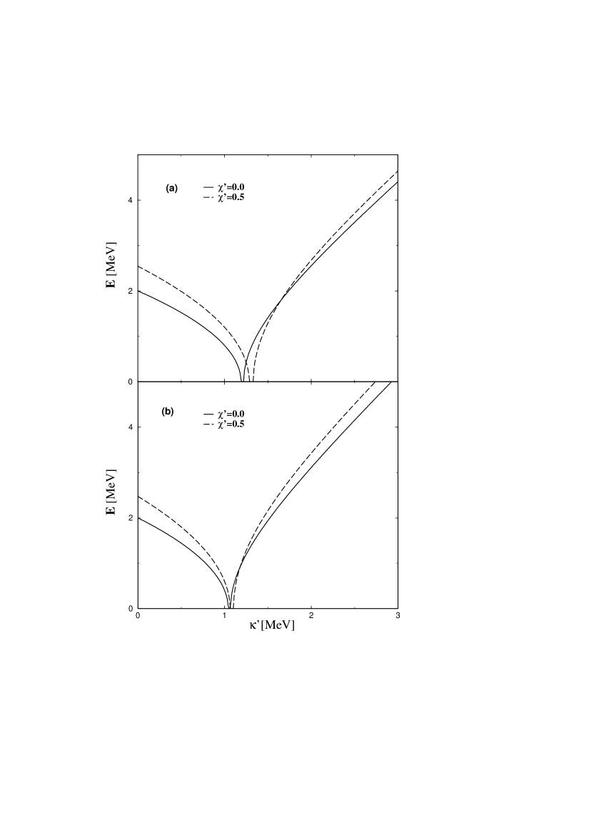
FIG. 1.: The energies of the harmonic modes corresponding to the VP1 (left branch) and VP2 (right branch) defined in eqs. (2.7) and (2.8) are plotted as functions of the proton-neutron pairing strength (eqs. (2.2) and (2.11)) k’ for the mother (a) and the daughter (b) nuclei. Energies as well as strength $\chi^{\prime}$ are given in units of MeV

FIGURE 2

FIG. 2.: Energies of the harmonic modes corresponding to VP3 (point and dashed-point lines) and VP4 (full and dashed lines) are given in units of MeV as functions of proton-neutron pairing strength k’

FIGURE 3

FIG. 3.: The double beta Fermi transition amplitudes obtained with the initial, intermediate and final states provided by VP1 (full line) VP2 (dashed line) formalism (a) and by diagonalizing the limit $\Omega$ goes to infinity of the HP boson expanded Hamiltonian (b) are given as function of the particle-particle interaction strength k’.

FIGURE 4

FIG. 4.: The double beta transition amplitude obtained by considering the states for mother, daughter and intermediate odd-odd nuclei as eigenstates of the Holstein-Primakoff boson expanded Hamiltonian (full line) and of the first order truncated HP Hamiltonian (dashed line) as function of the proton-neutron pairing strength k’ defined as in eq. (2.11)

FIGURE 5

FIG. 5.: The transition amplitude for double beta Fermi decay calculated with the standard pnQRPA (long dashed line), pnQRPA plus the second order corrections(dashed line) and pnQRPA plus second and third order corrections (dashed-point-point line)in the transition operator is represented as function of k’. For comparison the exact result is also presented (full line).

FIGURE 6

FIG. 6.: The transition amplitude from the ground state of the mother nucleus to the two pairing vibrational states, characterizing the daughter nucleus, is plotted as a function of the proton-neutron pairing strength k’.

FIGURE 7

FIG. 7.: The first five eigenvalues of the Holstein-Primakoff boson expanded Hamiltonian (4.4), for mother (a) and daughter (b) nuclei, are represented as functions of k’.

FIGURE 8

FIG. 8.: The absolute values for the leading two amplitudes of the first four eigenstates of the Holstein-Primakoff boson expanded Hamiltonian given by Eq. (4.4) are represented as functions of k’. In the upper panel the 1st and 3rd eigenstates are analyzed while in the lower panel the 2nd and the 4th are given.

FIGURE 9

FIG. 9.: The norms of the states defined by eqs.. (5.1),(5.2),(5.4),(5.5) are plotted as functions of the proton-neutron pairing strength k’.

FIGURE 10

FIG. 10.: The exponent $\stackrel{{\scriptstyle\circ}}{{\alpha}}_{k}$ entering the definition of the states $|\Phi_{k}\rangle$ given by Eq. (5.7).

FIGURE 11

FIG. 11.: The weights for a two phonon state in the structure of the states $|\Phi_{k}\rangle$ are plotted as function of the strength of the particle particle interaction.

REFERENCES

- [1] W. C. Haxton and G. J. Stephenson, Jr., Prog. Part. Nucl. Phys. 12 (1984) 409.
- [2] M. Doi, T. Kotani and E. Takasugi, Prog. Theor. Phys., Suppl. 83 (1985) 1.
- [3] A. Faessler, Prog. Part. Nucl. Phys. 21 (1988) 2139.
- [4] T. Tomoda, Rep. Prog. Phys. 54(1991) 53.
- [5] J. Suhonen, O. Civitarese, Phys. Rep. 300 (1998) 2139.
- [6] A. Faessler and F. Šimkovic, J. Phys. G 24(1998) 2139.
- [7] P. Vogel and P. Fischer, Phys. Rev. C 32 (1985) 1362.
- [8] P. Vogel and M. R. Zirnbauer, Phys. Rev. Lett. 57 (1986) 3148 .
- [9] O. Civitarese, A. Faessler and T. Tomoda, Phys. Lett. B 194 (1986) 11.
- [10] K. Grotz, H. V. Klapdor and J. Metzinger, Phys. Lett. B 132 (1983) 22.
- [11] H. V. Klapdor and K. Grotz, Phys. Lett. B 142 (1984) 323.
- [12] K. Muto, E. Bender and H. V. Klapdor, Z. Phys. A 334, (1989) 177.
- [13] J. Suhonen, T. Taigel and A. Faessler, Nucl. Phys.A486 (1988) 91.
- [14] A. A. Raduta, A. Faessler, S. Stoica and W. Kaminski, Phys. Lett. B 254 (1991) 7 .
- [15] A. A. Raduta, A. Faessler and S. Stoica, Nucl. Phys. A 534 (1991) 149.
- [16] J. Suhonen, Nucl. Phys. A 563 (1993) 205 .
- [17] A. Griffiths and P. Vogel, Phys. Rev. C 46 (1992) 181.
- [18] A. A. Raduta and J. Suhonen, Phys. Rev. C53 (1996) 176.
- [19] A. A. Raduta and J. Suhonen, J. Phys. G N. Ph. 22 (1996) 123.
- [20] F. Šimkovic, A. A. Raduta, M. Veselsky, A. Faessler, Phys. Rev. C 61 (2000) 044319.
- [21] J. Toivanen, J. Suhonen, Phys. Rev. Lett.75 (1995) 410.
- [22] J. Schwieger, F. Šimkovic and A. Faessler, Nucl. Phys.A600 (1996) 179.
- [23] J. Schwieger F. Šimkovic, A. Faessler and W. A. Kaminski, J. Phys. G 23 (1997) 1647; Phys. Rev. C57 (1998) 1738.
- [24] A.A. Raduta, M.C. Raduta, A. Faessler,W. Kaminski, Nucl. Phys.A 634(1998) 497.
- [25] A. A. Raduta, F. Šimkovic, A. Faessler, Jour. Phys. G 26(2000) 793.
- [26] A. A. Raduta, O. Haug, F. Šimkovic, A. Faessler, Nucl. Phys. A 671 (2000) 255.
- [27] A. A. Raduta, O. Haug, F. Šimkovic, A. Faessler, Jour. Phys. G 26 (2000) 1327.
- [28] A. A. Raduta, L. Pacearescu, V. Baran, P.Sariguren and E. Moya de Guerra, Nucl. Phys. A 675 (2000) 503.
- [29] M. Sambataro and J. Suhonen, Phys. Rev. C56 (1997) 782.
- [30] J. G. Hirsch, P. O. Hess and O. Civitarese, Phys. Rev. C 56 (1997) 199.
- [31] O. Civitarese, P. O. Hess, J. G. Hirsch and M. Reboiro, C 59 (1999) 194.
- [32] A. A. Raduta, D. S. Delion and Amand Faessler, Phys. Rev. C 51 (1995) 3008.
- [33] A. A. Raduta, D. S. Delion and Amand Faessler, Nucl. Phys. A 617 (1997) 176.
- [34] T. Holstein and H. Primakoff, Phys. Rev 58 (1940) 1098.
- [35] J. Schwinger ”On angular momentum” in Quantum Theory of Angular Momentum, 1965, edited by L. Biedenharn H. Van Dam (Academic, New York), p. 229.