A correlated model for $\Lambda$–hypernuclei

Abstract

We study the properties of hypernuclei containing one $\Lambda$ hyperon in the framework of the correlated basis function theory with Jastrow correlations. Fermi hypernetted chain integral equations are derived and used to evaluate energies and one–body densities of $\Lambda$–hypernuclei having a doubly closed shell nucleonic core in the $jj$ coupling scheme, from Carbon to Lead. We also study hypernuclei having the least bound neutron substituted by the $\Lambda$ particle. The semi-realistic Afnan and Tang nucleon-nucleon potential and Bodmer and Usmani $\Lambda$-nucleon potential are adopted. The effect of many–body forces are considered by means either of a three body $\Lambda$-nucleon-nucleon potential of the Argonne type or of a density dependent modification of the $\Lambda$-nucleon interaction, fitted to reproduce the $\Lambda$ binding energy in nuclear matter. While Jastrow correlations underestimate the attractive contribution of the three body $\Lambda$ interaction, the density dependent potential provides a good description of the $\Lambda$ binding energies over all the nuclear masses range, in spite of the relative simplicity of the model.

I Introduction

The microscopic study of atomic nuclei has gained in the recent years a noticeable level of reliability, following the improved knowledge of the interaction between the nucleons and the development of new and more sophisticated many–body theories. It is now possible to exactly solve the Schrödinger equation for nuclei containing up to $A=8$ nucleons[1], while the structure of medium and heavy nuclei can be to a large extent understood by means either of variational techniques[2] or of highly refined perturbative expansions[3]. These relatively recent developments have clearly stressed several inadequacies of the independent particle model (IPM), on which the time honoured shell model is based. For instance, the IPM completely fails in describing the large energy behaviour of the one nucleon momentum distribution and the quenching of the spectroscopic factors[4].

The scenario is not equally bright for hypernuclei, or bound systems of nucleons and one or more strange baryons, as the $\Lambda$ or $\Sigma$ hyperons. The many–body techniques developed for the nuclei can be, in most of the cases, straightforwardly extended to the hypernuclei, at least from a formal point of view. However, the weak point of a consistent microscopic approach now lies in the poorer understanding of the hyperon–nucleon (YN) and hyperon–hyperon (YY) interactions with respect to the nuclear case. The limited amount of information on the YN scattering data is a consequence of the experimental difficulties due to the short lifetime of the hyperons and to the low intensity of the beam fluxes. For this reason phenomenological models and effective YN interactions have been often used in the study of hypernuclei. Approaches based upon Skyrme interactions [5] and Woods–Saxon [6] potentials as well as relativistic mean field theories [7, 8, 9] have been used. However, also microscopic YN potentials have been recently produced [10, 11, 12] and adopted to study the structure of hypernuclei from ${}^{17}_{~{}\Lambda}$O to ${}^{208}_{~{}~{}\Lambda}$Pb [13, 14]. The $\Lambda$ single–particle properties have been investigated in details in Ref. [15], making use of the nuclear matter Fermi hypernetted chain results in a local density approximation.

In this paper we present a microscopic study of the structure of various hypernuclei containing a single $\Lambda$ hyperon. This study has been done by extending the correlated basis functions theory and the Fermi hypernetted chain (FHNC) equations technique [16] to describe nucleonic systems containing one hyperonic impurity. The nucleon–nucleon (NN) interaction we have chosen is the semi-realistic two–nucleon S3 potential of Afnan and Tang [17], as modified in Ref.[18]. In the present work we neglect the three–nucleon potential. For the $\Lambda$–nucleon ($\Lambda$N) potential we have chosen that proposed by Bodmer and Usmani [19]. We have investigated the effects of many-body forces involving the $\Lambda$ by explicitly considering a $\mbox{$\Lambda$}NN$ interaction or, alternatively, by including a density dependence in the bare $\mbox{$\Lambda$}N$ force.

The interactions generate strong NN and $\Lambda$N correlations, beyond those described by a mean field approach. In our work the correlation effects are accounted for by a Jastrow correlated wave function, where the two–body correlations depend on the interparticle distances only. More realistic hamiltonians demand for a strong spin and isospin dependence in the correlation factor. However, we consider the simple Jastrow ansatz as a first step towards a more complete description of the hypernuclei. The same strategy has been followed for doubly closed shell nuclei, where the accuracy of the variational method has now reached the same level as in nuclear matter[20].

The FHNC equations for a $\Lambda$ embedded in infinite nuclear matter were developed in Ref.[21]. In Ref.[22], doubly closed shell nuclei in $ls$–coupling were studied by FHNC and Jastrow–type correlations, while the $jj$–coupling was introduced in such a scheme in Ref.[23]. It was so possible to study nuclei ranging from ¹²C to ²⁰⁸Pb within the correlated basis function theory, using cluster expansion at all orders and avoiding such shortcuts as low order cluster truncations and local density approximations. The results obtained in those papers are the basis of the present FHNC study of $\Lambda$–hypernuclei.

The plan of the paper is as follows: section II is devoted to a brief description of the hamiltonian and of the correlated wave function; section III gives an outline of the FHNC theory for the hypernucleus; in section IV the expressions for the variational energy are presented and discussed; the results are given in section V and the conclusions are drawn in section VI.

II Hamiltonian and trial wavefunctions.

The system under study is a hypernucleus composed by $A$ nucleons and one $\Lambda$ hyperon. The formalism we have developed is however general enough to describe any nuclear systems containing a non-nucleonic particle, treated as an impurity in the nucleonic fluid.

We write the hamiltonian of the system as:

$$H_{N+\Lambda} = H_{N}+H_{\Lambda}=$$ (3)

$$-\sum_{i=1}^{A}\frac{\hbar^{2}}{2m_{i}}\nabla^{2}_{i}+\sum_{j>i=1}^{A}V^{NN}(i,j)$$

$$-\frac{\hbar^{2}}{2m_{\Lambda}}\nabla^{2}_{\Lambda}+\sum_{i=1}^{A}V^{\Lambda N}(\Lambda,i)+\sum_{j>i=1}^{A}V^{\Lambda NN}_{3}(\Lambda,i,j)~{},$$

where we have considered two– and three–body interactions between the hyperon and the nucleons and only two–body ones between the nucleons. In the hamiltonian (3) the purely nucleonic part, $H_{N}$, has been separated from that involving the $\Lambda$, $H_{\Lambda}$. The separation will be useful in the remainder of the paper.

As already stated in the introduction, we use the modified NN S3 potential, which is fixed to reproduce the $s$ wave scattering nucleon-nucleon phase shifts at low energies, gives reasonable results both for light nuclei and nuclear matter and allows for utilizing only central two–body correlations between the nucleons. The operatorial structure of S3 is:

$$V^{NN}(i,j)=\sum_{p=1}^{4}V^{p}(r_{ij})O^{p}_{ij}~{},$$ (4)

where $O^{p=1-4}_{i,j}=1$, $\mbox{\boldmath$\sigma$}_{i}\cdot\mbox{\boldmath$\sigma$}_{j}$, $\mbox{\boldmath$\tau$}_{i}\cdot\mbox{\boldmath$\tau$}_{j}$, $\mbox{\boldmath$\sigma$}_{i}\cdot\mbox{\boldmath$\sigma$}_{j}\mbox{\boldmath$\tau$}_{i}\cdot\mbox{\boldmath$\tau$}_{j}$. Modern nucleon-nucleon potentials are more complicated and contain the essential tensor terms, absent in S3. On the other hand, we are mainly interested in presenting and testing the formalism. Adopting the S3 potential is sufficient for this purpose and has the advantage of avoiding the technical complications deriving from the use of more realistic potentials.

Within the same philosophy, we have chosen the $\Lambda$–nucleon potential proposed by Bodmer and Usmani [19]. This potential has central, spin and space–exchange components:

$$V^{\Lambda N}(1,2)=V^{1}_{\Lambda N}(r_{12})+V^{2}_{\Lambda N}(r_{12})\mbox{\boldmath$\sigma$}_{\Lambda}\cdot\mbox{\boldmath$\sigma$}_{N}+V^{x}_{\Lambda N}(r_{12})P_{x}~{},$$ (5)

with

$$V^{1}_{\Lambda N}(r) = v_{0}(r)\left(1-\epsilon\right)~{},$$ (6)

$$V^{2}_{\Lambda N}(r) = \frac{1}{4}(v_{s}-v_{t})T_{\pi}^{2}(r)~{},$$ (7)

$$V^{x}_{\Lambda N}(r) = \epsilon~{}v_{0}(r)~{},$$ (8)

where $P_{x}$ is the spatial exchange operator and $v_{0}$ is defined as:

$$v_{0}(r)=\frac{W_{c}}{1+\exp(\frac{r-R}{a})}-\frac{1}{4}(v_{s}+3v_{t})T_{\pi}^{2}(r)\,\,\,.$$ (9)

The one-pion exchange term is

$$T_{\pi}(r)=\left(1+\frac{3}{\mu r}+\frac{3}{(\mu r)^{2}}\right)\frac{e^{-\mu r}}{\mu r}\left(1-e^{-cr^{2}}\right)^{2}\,\,\,,$$ (10)

with the pion mass $\mu$=0.7 fm^-1 and the cutoff parameter $c$=2.0 fm^-2. The values of the various parameters $v_{s},v_{t},\epsilon,W_{c},R,a$ are given in Ref. [24]. In this reference, a three-body $\Lambda$-nucleon-nucleon interaction was added to the just described $\Lambda$-nucleon one in order to fit the hypernucleus ${}^{17}_{~{}\Lambda}O$ empirical $B_{\Lambda}$ by the variational Monte Carlo (VMC) method. The $\mbox{$\Lambda$}NN$ interaction has an important, attractive two-pion exchange part, which is the source of a tensor term. The tensor contribution, however, results to be zero if simple central correlations are adopted. As a consequence, such a semi-microscopic $\mbox{$\Lambda$}NN$ interaction is too repulsive in a Jastrow correlated model, as we shall discuss later. For this reason, we simulate the effects of three– and more–body potentials by using an approach similar to that developed by Friedman and Pandharipande for pure nucleonic matter [25]. We multiply $V^{\mbox{$\Lambda$}N}(1,2)$ by a density dependent function

$$F_{\rho}(1,2)=\exp\{-\gamma[\rho(r_{1})+\rho(r_{2})]/2\}~{},$$ (11)

where $\rho(r)$ is the nucleonic density. The value of the parameter $\gamma$ is fixed to reproduce the empirical value of a single $\Lambda$ binding energy in nuclear matter, $B_{\Lambda}^{NM}=30$ MeV.

The binding energy of the $\Lambda$ particle is defined as minus the difference between the energies of the nuclear systems with and without the $\Lambda$ :

$$-B_{\Lambda} = \frac{1}{2j+1}\sum_{m}<H_{N+\Lambda}>_{A+\Lambda}-<H_{N}>_{A}$$ (13)

$$-\left(\frac{1}{2j+1}\sum_{m}<T^{cm}_{N+\Lambda}>_{A+\Lambda}-<T^{cm}_{N}>_{A}\right)~{},$$

where we have used the notation:

$$<X>_{Y}=\frac{1}{<\Psi_{Y}|\Psi_{Y}>}\int d\mbox{\boldmath$\tau$}\Psi^{*}_{Y}X\Psi_{Y}~{},$$ (14)

with $Y=A+\mbox{$\Lambda$}$ or $A$. In the previous equations we have averaged on the third component of the $\Lambda$ total angular momentum and we have explicitly singled out the difference between the center of mass energies of the two systems.

Our approach is based upon the variational principle, therefore the energy functionals given in eq.(13), $<H_{N+\Lambda}>_{A+\Lambda}$ and $<H_{N}>_{A}$, should be independently minimized with respect to variations of the many-body wavefunctions, $\Psi_{Y}$. The hypernucleus wavefunction is chosen as:

$$|\Psi_{A+\Lambda}>=\left(\prod_{i=1}^{A}f_{\Lambda}(r_{\Lambda i})\right)\phi_{nljm}^{\Lambda}({\bf r}_{\Lambda})|\Psi_{A}>~{},$$ (15)

where $\phi_{nljm}^{\Lambda}$ is the mean-field single particle wavefunction of the $\Lambda$ in $jj$–coupling, $f_{\Lambda}(r_{\Lambda i})$ is a two-body scalar (Jastrow) correlation between the hyperon and a single nucleon and $|\Psi_{A}>$ is the correlated wave function describing the remaining $A$ nucleons. In our calculation this function is defined as:

$$|\Psi_{A}>=\left(\prod_{j>i=1}^{A}f_{N}(r_{ij})\right)\Phi_{N,Z}(1,\ldots,A)~{},$$ (16)

where $\Phi_{N,Z}$ is the Slater determinant of a set of single particle wave functions of $N$ neutrons and $Z$ protons. Obviously, $A=Z+N$.

III Densities and FHNC equations

The energy expectation values are evaluated by means of the Fermi hypernetted chain[16] cluster diagrams resummation technique. As already mentioned, our approach consists in considering the $\Lambda$ as an impurity in the nucleonic fluid. The FHNC equations for an impurity in homogeneous matter were derived in Ref. [21] for a $\Lambda$ hyperon in symmetric nuclear matter and in Refs. [26, 27] for a ⁴He atomic impurity in liquid ³He.

Our aim is the evaluation the $\Lambda$ binding energy in finite nuclear systems. To this purpose, we extend the FHNC equations developed in Ref.[23] for doubly closed shell nuclei in the $jj$–coupling scheme with a Jastrow correlated wave functions.

The basic quantities to be analyzed are the one- and two-body densities (OBD and TBD). It is convenient to define densities for each type of particle, protons $p$, neutrons $n$ and $\Lambda$:

$$\rho_{1,A+\Lambda}^{\alpha}({\bf r}) = \langle\sum_{k=1}^{A}\delta({\bf r}-{\bf r}_{k})P^{\alpha}_{k}\rangle_{A+\Lambda}$$ (17)

$$\rho_{1}^{\Lambda}({\bf r}) = \langle\delta({\bf r}-{\bf r}_{\Lambda})\rangle_{A+\Lambda}$$ (18)

where $\alpha=p,n$, $P^{\alpha}$ is the projector operator over the particle of $\alpha$ type. An averaged sum on the third components of the $\Lambda$ particle angular momentum is understood. As in Refs.[22, 23] the densities are evaluated by using cluster expansion techniques. The nucleonic OBD are divided in two parts:

$$\rho_{1,A+\Lambda}^{\alpha}({\bf r})=\rho_{1,A}^{\alpha}({\bf r})+\rho_{1,\Lambda}^{\alpha}({\bf r}).$$ (19)

The first part is given by the sum of the cluster diagrams containing only nucleons, and represents the nuclear bulk contribution to the OBD. One of the diagrams contributing to this part is the $A$ diagram of Fig.1. The second part of eq. 19, called rearrangement term, is obtained by summing all the diagrams containing the $\Lambda$ as an internal particle, like the diagram $B$ of Fig.1, and provides the modification of the nucleon OBD due to the presence of the $\Lambda$ impurity. A mean-field description of the hypernucleus does not provide any rearrangement term. Finally, the diagrams where the $\Lambda$ is an external particle, like the $C$ diagram of Fig.1, are summed in the $\Lambda$-OBD, $\rho_{1}^{\Lambda}({\bf r})$. The separation of the one-body densities in bulk, rearrangement and $\Lambda$ terms will be very useful for the calculation of the $\Lambda$ binding energy in the nucleus and it will be exploited also for the calculation of other quantities occurring in the FHNC scheme.

In analogy with the one–body densities, we define the two–body densities as:

$$\rho_{2,q,A+\Lambda}^{\alpha\beta}({\bf r},{\bf r}^{\prime}) = \langle\sum_{k\neq l=1}^{A}\delta({\bf r}-{\bf r}_{k})\delta({\bf r}^{\prime}-{\bf r}_{l})O^{q}_{kl}P^{\alpha}_{k}P^{\beta}_{l}\rangle_{A+\Lambda}$$ (20)

$$= \rho_{2,q,A}^{\alpha\beta}({\bf r},{\bf r}^{\prime})+\rho_{2,q,\Lambda}^{\alpha\beta}({\bf r},{\bf r}^{\prime})~{},$$ (21)

where $\alpha,\beta=p,n$ and $O^{q}_{kl}$ is one of the operators defined in eq.(4). The $\Lambda$N two–body densities are defined as:

$$\rho_{2,q}^{\Lambda\alpha}({\bf r},{\bf r}^{\prime}) = \langle\delta({\bf r}-{\bf r}_{\Lambda})\sum_{k=1}^{A}\delta({\bf r}^{\prime}-{\bf r}_{k})O^{q}_{\Lambda k}P^{\alpha}_{k}\rangle_{A+\Lambda}~{},$$ (22)

$$\rho_{2,x}^{\Lambda\alpha}({\bf r},{\bf r}^{\prime}) = \langle\delta({\bf r}-{\bf r}_{\Lambda})\sum_{k=1}^{A}\delta({\bf r}^{\prime}-{\bf r}_{k})P_{x}P^{\alpha}_{k}\rangle_{A+\Lambda}~{},$$ (23)

where $O^{q}_{\mbox{$\Lambda$}k}=1,~{}\mbox{\boldmath$\sigma$}_{\Lambda}\cdot\mbox{\boldmath$\sigma$}_{k}$ are the operators of the $\Lambda$N interaction (5), and $P_{x}$ is the space exchange operator between the $\Lambda$ and the k-nucleon.

In the FHNC approach the TBD are described in terms of two-body correlation functions $f_{N}(r_{kl})$ and $f_{\Lambda}(r_{\Lambda k})$, and of uncorrelated densities. The latter are built from a single particle basis, defined in the present paper as a set of $jj$ coupled wave functions of the type:

$$\phi_{k}^{t}(x)\equiv\phi^{t}_{nljm}({\bf r})=R^{t}_{nlj}(r)\sum_{\mu,s}<l\mu\frac{1}{2}s|jm>Y_{l,\mu}(\widehat{r})\chi_{s}~{},$$ (24)

where $t=p,n,\mbox{$\Lambda$}$. $Y_{l,\mu}$ are the spherical harmonics, $<l\mu\frac{1}{2}s|jm>$ are the Clebsch–Gordan coefficients and $\chi_{s}$ the two-component Pauli spinors.

In the nucleonic case, the uncorrelated two–body densities are:

$$\rho_{0}^{\alpha}({\bf r}_{1},{\bf r}_{2}) = \sum_{k}\phi_{k}^{\alpha*}({\bf r}_{1})\phi_{k}^{\alpha}({\bf r}_{2})$$ (25)

$$= \sum_{s,s^{\prime}}\rho^{s,s^{\prime},\alpha}_{0}({\bf r}_{1},{\bf r}_{2})\chi_{s}^{\dagger}(1)\chi_{s^{\prime}}(2)~{}.$$ (26)

The explicit expressions of the parallel, $s=s^{\prime}$, and antiparallel $s=-s^{\prime}$ densities are given in Ref. [23] together with the other purely nucleonic FHNC quantities.

We briefly discuss here the quantities involving the $\Lambda$. The uncorrelated $\Lambda$ one–body density is given by:

$$\rho^{\Lambda}_{0}({\bf r})=\frac{1}{2j+1}\sum_{m}\phi^{\Lambda*}_{nljm}({\bf r})\phi^{\Lambda}_{nljm}({\bf r})=\frac{1}{4\pi}\left(R^{\Lambda}_{nlj}(r)\right)^{2}~{}.$$ (27)

The one-body $\Lambda$ uncorrelated density matrix is needed to calculate diagrams where the spatial coordinates between the $\Lambda$ and one nucleon are exchanged. Its expression is:

$$\rho^{\Lambda}_{0}({\bf r}_{1},{\bf r}_{2})=\frac{1}{4\pi}R^{\Lambda}_{nlj}(r_{1})R^{\Lambda}_{nlj}(r_{2})P_{l}(\cos\theta_{12})~{},$$ (28)

where we have indicated with $P_{l}$ the Legendre polynomial of $l$th degree and $\theta_{12}$ the angle between the two vectors.

A detailed description of the FHNC equations in the nucleonic matter, in a $jj$ coupled single particle basis computational scheme, has been done in Ref. [23]. We do not give here the equations for this case, but we rather present and discuss the changes related to the presence of the $\Lambda$. The FHNC $\Lambda$–densities are:

$$\rho_{1}^{\Lambda}(r) = \xi_{d}^{\Lambda}(r)=\xi_{e}^{\Lambda}(r)\rho_{0}^{\Lambda}(r)~{},$$ (29)

$$\xi_{e}^{\Lambda}(r) = \frac{1}{C_{\Lambda}}\exp[U_{d}^{\Lambda}(r)]~{},$$ (30)

$$C_{\Lambda} = \int d{\bf r}~{}\rho_{0}^{\Lambda}(r)~{}\exp[U_{d}^{\Lambda}(r)]~{},$$ (31)

$$\rho_{2,1}^{\Lambda\beta}({\bf r}_{1},{\bf r}_{2}) = \xi_{d}^{\Lambda}(r_{1})\left(\xi_{d}^{\beta}(r_{2})g_{dd}^{\Lambda\beta}({\bf r}_{1},{\bf r}_{2})+\xi_{e}^{\beta}(r_{2})g_{de}^{\Lambda\beta}({\bf r}_{1},{\bf r}_{2})\right)~{},$$ (32)

$$\rho_{2,2}^{\Lambda\beta}({\bf r}_{1},{\bf r}_{2}) = 0~{}.$$ (33)

The functions $\xi_{d,e}^{\Lambda}(r)$, $U_{d}^{\Lambda}(r)$ and $g^{\Lambda\beta}_{xy}({\bf r}_{1},{\bf r}_{2})$ are analogous to their nucleonic partners whose expressions are given in the Appendices A and B of Ref. [23], and they are obtained with the substitution $\alpha\rightarrow\Lambda$. In extending the expressions given in the reference, we should remember that there is no sum on $\Lambda$, since it is just a single external impurity, and that we consider the same correlation function between $\Lambda$ and any type of nucleon: $f_{\Lambda\beta}(r_{12})=f_{\Lambda}(r_{12})$ with $\beta=p,n$.

Eq.(33) shows that, in our case, the spin component of the two-body density, $\rho_{2,2}^{\Lambda\beta}$, is zero. The reason lies in the fact that only diagrams corresponding to exchanges between identical particles contribute to the spin component of the two–body density for Jastrow correlated wave functions. As a consequence they do not affect the $\Lambda$N–TBD. Direct diagrams, where the particles are not exchanged, may contribute to $\rho_{2,2}^{\Lambda\beta}$ only if the correlation contains spin dependent components (which is not our case). Moreover, this type of contribution has been found to be generally small [24].

The evaluation of the diagrams containing the space exchange $\Lambda$N potential requires the introduction of a space exchange density, given by:

$$\rho_{2,x}^{\Lambda\alpha}({\bf r},{\bf r}^{\prime})=\frac{2}{C_{\Lambda}}f_{\Lambda}^{2}(|{\bf r}-{\bf r}^{\prime}|)\rho^{\Lambda}_{0}({\bf r},{\bf r}^{\prime})\rho^{ss\alpha}({\bf r},{\bf r}^{\prime})~{},$$ (34)

where $\rho^{ss\alpha}({\bf r},{\bf r}^{\prime})$ is defined as in Appendix B of [23], with the substitutions $f_{\alpha\beta}(r_{12})\rightarrow f_{\Lambda}(r_{12})f_{N}(r_{12})$ in the construction of the $g_{\omega d}$ functions.

The expressions of the rearrangement terms are quite lengthy since the $\Lambda$ may be present in any of the elements involved in the densities. We give below the expression of the contributions to the one–body density:

$$\rho_{1,\Lambda}^{\alpha}(r) = \left(U_{d,\Lambda}^{\alpha}(r)\left[\rho_{0}^{\alpha}(r)+U_{e}^{\alpha}(r)\right]+U_{e,\Lambda}^{\alpha}(r)\right)~{}\exp[U_{d}^{\alpha}(r)]$$ (35)

$$= \xi_{d}^{\alpha}(r)U_{d,\Lambda}^{\alpha}(r)+\xi_{e}^{\alpha}(r)U_{e,\Lambda}^{\alpha}(r)=\xi_{d,\Lambda}^{\alpha}(r)~{},$$ (36)

$$\xi_{e,\Lambda}^{\alpha}(r) = U_{d,\Lambda}^{\alpha}(r)~{}\exp[U_{d}^{\alpha}(r)]~{}.$$ (37)

The $U_{X=d,e}^{\alpha}$ functions are given in Ref.[23], while the $U_{X,\Lambda}^{\alpha}$ and the rearrangement parts of the two–body densities are given in the Appendix.

IV The variational energy

In this section we discuss the evaluation of the variational energy of a $\Lambda$ hypernucleus in the framework of the FHNC approach. The potential energy is separated into its nucleonic and $\Lambda$ pieces:

$$<V_{N+\Lambda}>_{A+\Lambda}=<V_{N}>_{A+\Lambda}+<V_{\Lambda}>_{A+\Lambda}~{}.$$ (38)

The expectation values can be expressed in terms of the two–body distribution functions as:

$$<\overline{V}_{N}>_{A+\Lambda} = \frac{1}{2}\sum_{\alpha,\beta=p,n}\sum_{q=1}^{4}\int d{\bf r}_{1}d{\bf r}_{2}V^{q}(r_{12})\rho_{2,q,A+\Lambda}^{\alpha\beta}({\bf r}_{1},{\bf r}_{2})$$ (39)

$$=\ \ \ <V_{N}>_{A} + \frac{1}{2}\sum_{\alpha,\beta=p,n}\sum_{q=1}^{4}\int d{\bf r}_{1}d{\bf r}_{2}V^{q}(r_{12})\rho_{2,q,\Lambda}^{\alpha\beta}({\bf r}_{1},{\bf r}_{2})~{}~{},$$ (40)

$$<\overline{V}_{\Lambda}>_{A+\Lambda} = \sum_{\alpha=p,n}\sum_{q=1}^{2}\int d{\bf r}_{1}d{\bf r}_{2}V^{q}_{\Lambda N}(r_{12})\rho_{2,q}^{\Lambda\alpha}({\bf r}_{1},{\bf r}_{2})+$$ (42)

$$\sum_{\alpha=p,n}\int d{\bf r}_{1}d{\bf r}_{2}V^{x}_{\Lambda N}(r_{12})\rho_{2,x}^{\Lambda\alpha}({\bf r}_{1},{\bf r}_{2})~{},$$

where $<\overline{V}>$ indicates the average on the third components of the $\Lambda$ angular momentum and $<V_{N}>_{A}$ is the bulk nucleonic potential energy.

Because the minimizations of $<H_{N+\Lambda}>_{A+\Lambda}$ and $<H_{N}>_{A}$ must be, in principle, carried on independently, the nucleon–nucleon Jastrow correlation, $f_{N}(r)$, might be different in the two cases, as well as the nucleon single particle wave functions, $\phi_{k}({\bf r})$. However, we found that in our cases $f_{N}(r)$ and $\phi_{k}({\bf r})$ do not practically change in going from the $A$ to the $A+\Lambda$ system. As a consequence, in our approach the nucleonic part of the hypernucleus wave function has been kept the same as in nucleus. This fact allows for obtaining the potential energy contribution to the binding energy of the $\Lambda$ by subtracting the pure nucleus $<V_{N}>_{A}$ from $<\overline{V}_{N}>_{A+\Lambda}$. The remaining part is separated in two contributions: the potential energy due to the interaction $\Lambda$–nucleon, or interaction energy, and the modifications of the nucleon–nucleon potential energy due to the presence of the $\Lambda$, or rearrangement energy. We put in evidence these contributions by rewriting:

$$V_{\Lambda}=<\overline{V}_{N+\Lambda}>_{A+\Lambda}-<V_{N}>_{A}=V_{\Lambda}^{I}+V_{\Lambda}^{R}~{},$$ (43)

with

$$V_{\Lambda}^{I}=\sum_{\alpha=p,n}\int d{\bf r}_{1}d{\bf r}_{2}\left(\sum_{q=1}^{2}V^{q}_{\Lambda N}(r_{12})\rho_{2,q}^{\Lambda\alpha}({\bf r}_{1},{\bf r}_{2})+V^{x}_{\Lambda N}(r_{12})\rho_{2,x}^{\Lambda\alpha}({\bf r}_{1},{\bf r}_{2})\right)~{},\\$$ (44)

and

$$V_{\Lambda}^{R}=\frac{1}{2}\sum_{\alpha,\beta=p,n}\sum_{q=1}^{4}\int d{\bf r}_{1}d{\bf r}_{2}V^{q}(r_{12})\rho_{2,q,\Lambda}^{\alpha\beta}({\bf r}_{1},{\bf r}_{2})~{}.$$ (45)

The separation in interaction and rearrangement terms can also be done for the $\Lambda$ kinetic energy, evaluated here by means of the Jackson–Feenberg expression [22]. Following an analysis similar to that done for the potential energy, we obtain:

$$T_{\Lambda}=<\overline{T}_{N+\Lambda}>_{A+\Lambda}-<T_{N}>_{A}=T_{\Lambda}^{I}+T_{\Lambda}^{R}~{}.$$ (46)

The interaction kinetic energy is given by:

$$T_{\Lambda}^{I} = -\frac{\hbar^{2}}{4m_{\Lambda}}\int d{\bf r}d\rho_{T1}^{\Lambda}({\bf r})\xi_{e}^{\Lambda}({\bf r})$$ (48)

$$-\frac{\hbar^{2}}{4}\left(\frac{1}{m}+\frac{1}{m_{\Lambda}}\right)\sum_{\alpha=p,n}\int d{\bf r}_{1}d{\bf r}_{2}~{}t[f_{\Lambda}(r_{12})]~{}\rho_{2,1}^{\Lambda\alpha}({\bf r}_{1},{\bf r}_{2})\,\,\,,$$

with

$$\rho^{\Lambda}_{T1}(r_{1})=\frac{1}{4\pi}\left[R^{\Lambda}_{nlj}(r_{1})\left(D^{\Lambda}_{nlj}(r_{1})-\frac{l(l+1)}{r^{2}_{1}}R^{\Lambda}_{nlj}(r_{1})\right)-\left(R^{\Lambda\prime}_{nlj}(r_{1})\right)^{2}\right]\,\,\,.$$ (49)

The expressions of $t[f_{\Lambda}]$ and $D^{\alpha}_{nlj}$ can be obtained from Ref.[23] (Eq.(16) and Appendix C).

The rearrangement part of the kinetic energy is:

$$T_{\Lambda}^{R} = -\frac{\hbar^{2}}{4m}\sum_{\alpha,\beta=p,n}\int d{\bf r}_{1}d{\bf r}_{2}t[f_{N}(r_{12})]\rho_{2,1,\Lambda}^{\alpha\beta}({\bf r}_{1},{\bf r}_{2})$$ (55)

$$-\frac{\hbar^{2}}{4m}\sum_{\alpha=p,n}\int d{\bf r}_{1}\rho_{T1}^{\alpha}({\bf r}_{1})\xi_{e,\Lambda}^{\alpha}({\bf r}_{1})$$

$$+\frac{\hbar^{2}}{4m}\sum_{\alpha=p,n}\int d{\bf r}_{1}d{\bf r}_{2}\rho_{T2}^{\alpha}({\bf r}_{1},{\bf r}_{2})\left[\xi_{e}^{\alpha}({\bf r}_{1})\xi_{e}^{\alpha}({\bf r}_{2})g_{dd,\Lambda}^{\alpha\alpha}({\bf r}_{1},{\bf r}_{2})+\right.$$

$$\left.\left(\xi_{e,\Lambda}^{\alpha}({\bf r}_{1})\xi_{e}^{\alpha}({\bf r}_{2})+\xi_{e}^{\alpha}({\bf r}_{1})\xi_{e,\Lambda}^{\alpha}({\bf r}_{2})\right)g_{dd}^{\alpha\alpha}({\bf r}_{1},{\bf r}_{2})\right]$$

$$-\frac{\hbar^{2}}{2m}\sum_{\alpha=p,n}\int d{\bf r}_{1}d{\bf r}_{2}\Bigl{[}\rho_{T3,P}^{\alpha}({\bf r}_{1},{\bf r}_{2})H_{cc,P,\Lambda}^{\alpha}({\bf r}_{1},{\bf r}_{2})$$

$$+\rho_{T3,A}^{\alpha}({\bf r}_{1},{\bf r}_{2})H_{cc,A,\Lambda}^{\alpha}({\bf r}_{1},{\bf r}_{2})\Bigr{]}~{},$$

where

$$H_{cc,D,\Lambda}^{\alpha}({\bf r}_{1},{\bf r}_{2})) = \xi_{e,\Lambda}^{\alpha}(r_{1})\Bigl{[}\xi_{e}^{\alpha}(r_{2})\left(\left(g_{dd}^{\alpha\alpha}({\bf r}_{1},{\bf r}_{2})-1\right)N_{cc,D}^{\alpha}({\bf r}_{1},{\bf r}_{2}))+N_{cc,D}^{(x)\alpha}({\bf r}_{1},{\bf r}_{2})\right)$$ (56)

$$+ \left(\xi_{e}^{\alpha}(r_{2})-1\right)N_{cc,D}^{(\rho)\alpha}({\bf r}_{1},{\bf r}_{2})+\xi_{e}^{\alpha}(r_{2})g_{dd}^{\alpha\alpha}({\bf r}_{1},{\bf r}_{2})E_{cc,D}^{\alpha}({\bf r}_{1},{\bf r}_{2})\Bigr{]}$$ (57)

$$+ \xi_{e}^{\alpha}(r_{1})\xi_{e,\Lambda}^{\alpha}(r_{2})g_{dd}^{\alpha\alpha}({\bf r}_{1},{\bf r}_{2})\left(N_{cc,D}^{\alpha}({\bf r}_{1},{\bf r}_{2})+E_{cc,D}^{\alpha}({\bf r}_{1},{\bf r}_{2})\right)$$ (58)

$$+ \xi_{e}^{\alpha}(r_{1})\Bigl{[}\xi_{e}^{\alpha}(r_{2})\Bigl{(}\left(g_{dd}^{\alpha\alpha}({\bf r}_{1},{\bf r}_{2})-1\right)N_{cc,D,\Lambda}^{\alpha}({\bf r}_{1},{\bf r}_{2})$$ (59)

$$+ g_{dd,\Lambda}^{\alpha\alpha}({\bf r}_{1},{\bf r}_{2})N_{cc,D}^{\alpha}({\bf r}_{1},{\bf r}_{2})+N_{cc,D,\Lambda}^{(x)\alpha}({\bf r}_{1},{\bf r}_{2})\Bigr{)}$$ (60)

$$+ \left(\xi_{e}^{\alpha}(r_{2})-1\right)N_{cc,D,\Lambda}^{(\rho)\alpha}({\bf r}_{1},{\bf r}_{2})$$ (61)

$$+ \xi_{e}^{\alpha}(r_{2})\left(g_{dd,\Lambda}^{\alpha\alpha}({\bf r}_{1},{\bf r}_{2})E_{cc,D}^{\alpha}({\bf r}_{1},{\bf r}_{2})+g_{dd}^{\alpha\alpha}({\bf r}_{1},{\bf r}_{2})E_{cc,D,\Lambda}^{\alpha}({\bf r}_{1},{\bf r}_{2})\right)\Bigr{]}.$$ (62)

Again the expressions of $\rho_{Tk}^{\alpha}$ for $k=1,2,3$ can be found in the appendix C of [23].

The difference of the center of mass kinetic energies is given by:

$$T_{\Lambda}^{cm}=-\frac{m_{\Lambda}}{Am+m_{\Lambda}}<T_{N}^{cm}>_{A}-\frac{\hbar^{2}}{4(Am+m_{\Lambda})}\int d{\bf r}_{1}\rho_{T1}^{\Lambda}({\bf r}_{1})~{},$$ (63)

and the expression of $<T_{N}^{cm}>_{A}$ is given in eq. (23) of Ref.[23].

V Results

We have studied the ground state structure of those $\Lambda$–hypernuclei having $N$ and $Z$ values corresponding to doubly closed shell nuclei in $jj$–coupling, ${}^{13}_{~{}\Lambda}$C, ${}^{17}_{~{}\Lambda}$O, ${}^{41}_{~{}\Lambda}$Ca, ${}^{49}_{~{}\Lambda}$Ca, ${}^{91}_{~{}\Lambda}$Zr and ${}^{209}_{~{}~{}\Lambda}$Pb. The same set of nuclei where the neutron in the highest neutron single particle level has been substituted by a $\Lambda$ hyperon (${}^{12}_{~{}\Lambda}$C, ${}^{16}_{~{}\Lambda}$O, ${}^{40}_{~{}\Lambda}$Ca, ${}^{48}_{~{}\Lambda}$Ca, ${}^{90}_{~{}\Lambda}$Zr and ${}^{208}_{~{}~{}\Lambda}$Pb) have been also considered. In order to deal in FHNC with the partially occupied neutronic level, we adopt the following procedure: the degeneracy factor $2j+1$, multiplying the partially occupied state contribution to the uncorrelated nucleonic OBD, has been replaced by the factor $2j$. In this way, the OBD results normalized to $A-1$. Moreover, in the spin parallel part of the uncorrelated nucleonic TBD, $\rho^{P}$, the $2j+1$ factor has been substituted by $2\sqrt{(2l+1)(2l+1/2)}-4l+2j-1$, while the (much smaller) antiparallel part, $\rho^{A}$, remains unchanged. This choice ensures a correct normalization of the TBD.

Two different mean field potentials have been used to build the single–particle nuclear wave functions. The first potential is a harmonic oscillator (HO) well with the same constant, $b_{N}$, for protons and neutrons; the second choice is the Woods–Saxon (WS) potential used in the calculations of Ref.[23]. The parameters of the WS potential are different for protons and neutrons. We have always used a harmonic oscillator potential for the $\Lambda$ single–particle potential.

The correlation functions have a gaussian form:

$$f_{X=\Lambda,N}(r)=1-\alpha_{X}\exp(-\beta_{X}r^{2})~{}.$$ (64)

In order to calculate $B_{\Lambda}$, we first minimize the bulk energy of the nucleus, $<H_{N}>_{A}$. The minimization has been performed for each nucleus in two ways, depending on the nucleonic single–particle used. In the case of the HO potential, the nuclear correlation, $f_{N}(r)$, has been taken from nuclear matter and the nucleus energy has been obtained by varying only the values of the oscillator constant of the HO mean field. For the Woods–Saxon case, the mean field potential has been kept fixed as in Ref. [23] and the parameters of the correlation have been varied. We consider the WS model as the most realistic one, since its parameters have been determined to reproduce at best the nuclear densities. It must be noticed that, in the region of the variational space corresponding to the energy minimum, the energy itself is rather insensitive to small changes of the WS parameters. Therefore it is possible to reproduce the densities and the radii without excessively spoiling the quality of the minimum.

For the description of the nucleonic part of the hypernucleus we take the same $f_{N}(r)$ and mean field potential as in the corresponding nucleus. Then, $<H_{N+\Lambda}>_{A+\Lambda}$ is minimized by changing only the $\Lambda$–HO constant and the parameters of the $\Lambda$–nucleon correlation function, $f_{\Lambda}(r)$.

The parameters of the nuclear correlation (64) with the HO mean field are $\alpha_{N}=0.7$ and $\beta_{N}=2.0$ fm^-2. The nuclear matter binding energy per nucleon with this correlation and the S3 potential, at saturation density ($\rho_{NM}=0.16$ fm^-3), is $B_{NM}$=14.43 MeV, close enough to the empirical value, $B_{NM,{\rm emp}}$=16 MeV, and comparable with the best, more sophisticated potentials on the market. For each nucleus the value of the oscillator constant, $b_{N}$, has been fixed to get the energy minimum. In Table I we compare our HO and WS binding energies and rms charge radii with their experimental values. A general reasonable agreement is found, considering the relative simplicity of both wave functions and interactions. In particular, the WS radii are close the experimental ones. The ¹²C nucleus represents somehow an anomaly, having a good estimate of the radius but a very small binding energy. The origin of this disagreement is still under investigation. It may be related to the inadequacy of a spherical model description of this nucleus.

The parameter $\gamma$ of the density dependent potential (DDP), described in Section II, has been chosen to reproduce the $\Lambda$ binding energy in nuclear matter, $B_{\Lambda,NM}$. We find $\gamma=2.2$ fm³ and $B_{\Lambda,NM}=30.26$ MeV and this value of the parameter $\gamma$ has been used in the remaining finite systems calculations. The parameters of the $\Lambda$–HO mean fields and of the $f_{\Lambda}(r)$ correlations at the $<H_{N+\Lambda}>_{A+\Lambda}$ minimum are shown in Table II.

In Table III we compare the contributions to the $\Lambda$ binding energy in the doubly closed shell hypernuclei calculated with the HO nucleonic mean field with those evaluated in nuclear matter We have also separated the interaction (I) and rearrangement (R) terms in the kinetic and potential energies. The upper part of the table gives the results with the two–body $\Lambda$N interaction only and the related $\Lambda$ binding energy, $B_{\Lambda}^{(2)}$. In the lower part of the table the contribution of the three-body $\Lambda$NN interaction of Ref.[24] and the corresponding binding energy $B_{\Lambda}^{(3)}$ are shown. Finally we present the results obtained with the DDP potential.

Since the empirical value of $B_{\Lambda}$ in ${}^{17}_{~{}\Lambda}$O is estimated to be about 13 MeV [24], the result obtained with the $\Lambda$N force only is too attractive. The VMC calculation of Ref. [24] gives $B_{\Lambda,{\rm VMC}}^{(2)}(^{17}_{~{}\Lambda}{\rm O})$=27.5$\pm$2.0 MeV, in qualitative agreement with our value. The empirical binding energy was reproduced in the VMC approach by the inclusion of an explicit $\Lambda$NN force. Using the same three–body potential, we obtain $B_{\Lambda}^{(3)}(^{17}_{~{}\Lambda}{\rm O})$=6.81 MeV. We have already pointed out that central, Jastrow, correlations underestimate the attractive contribution of the $\Lambda$NN interaction, as clearly appears from the $B^{(3)}_{\Lambda}$ value. This potential, when used in conjunction with Jastrow correlated wave functions, does not even bind the $\Lambda$ in heavy nuclei. Tensor–like correlations are needed in order to effectively use potentials induced by one– and more–pion exchanges in spherically symmetric systems[20]. The introduction of a DDP, fitted to the $\Lambda$ binding in nuclear matter, brings $B_{\Lambda}$ reasonably close to the empirical estimate, even with a relatively simple correlation. All the results presented hereafter have been obtained with the DDP.

In Table IV we give the binding energies of a $\Lambda$ in its $1s$ ground state, calculated with the HO single particle potential for several hypernuclei and nuclear matter. We explicitly show the overall interaction and rearrangement contributions. The difference of the center of mass kinetic energies has been included in the rearrangement part. The increase of the $\Lambda$ binding energy along A is mostly produced by the interaction energy and, specifically, by its potential energy part. In contrast, the dependence of the rearrangement energy on $A$ is much weaker. We found an analogous behavior the $\Lambda$ energies in the $1p$ and $1d$ states. To complete the information we give in Table V, the results for the $\Lambda$ energies in the $1p$ and $1d$ states with the nucleonic HO mean field. In Table VI we compare the $\Lambda$ binding energies obtained with a Woods–Saxon nucleonic mean field with the experimental energies. For the ${}^{90}_{~{}\Lambda}$Zr the comparison is done with the energies measured in ${}^{89}_{~{}\Lambda}$Y.

The results for the $\Lambda$ binding energies are summarized in Fig.2, where they are presented as a function of $A^{-2/3}$ and compared with the experimental energies of Refs. [29] (dots), [30] (triangles) and [31] for the ¹³C. The figure gives the $\Lambda$ energies in the $1s$, $1p$ and $1d$ states. The quality of the agreement with the experiment is rather good, in spite of the simplicity of the model. By inspecting the figure in more details, we find that all the calculations underbind the $\Lambda$ in Carbon by $\sim 30\%$, and provide a steeper variation of $B_{\Lambda}$ with respect to the experiments. This behavior resembles that already described in Carbon nucleus. It is also worth noticing that, as expected, the heavier nuclei, Zr and Pb, are better described by the Woods-Saxon well than by the HO one.

The effects of the $\Lambda$N correlations on the one–body densities are shown in Fig.3, where the proton densities in four nuclei are compared. The dotted lines are the IPM densities, the dashed lines are the densities obtained in a purely nucleonic FHNC calculations, and, finally, the full curves represent the proton densities obtained when a $\Lambda$ hyperon is added in the $s$ wave to the doubly magic nucleonic core. In general, correlation effects are more important in Oxygen and Calcium than in the other two nuclei. Moreover, the presence of the $\Lambda$ does not heavily modify the nucleonic densities. This is better shown in Fig.4, where the differences between proton (panel $a$) and neutron (panel $b$) densities with and without the $\Lambda$ are given. The differences shown in the figure have been amplified by a factor 1000. The heavier nuclei seem to be much more stable against deformations produced by the presence of the $\Lambda$.

This picture might change when the $\Lambda$ is inserted in the nucleonic core by substituting the last bound neutron. The differences, multiplied by 1000, between the nucleonic densities of the isotopic hypernuclei with A+1 and A hadrons are given in Fig.5. The panels show the differences between the protons (upper) and neutron (lower) densities. The conservation of the charge and mass numbers for each hypernucleus implies that the curves in the upper panel are normalized to zero, while those in the lower panel are normalized to one.

The analysis of this figure indicates that the nucleonic part is more perturbed if the $\Lambda$ substitutes a neutron having a low angular momentum, like in O, Ca, and Pb. In Zr the neutron modified into a $\Lambda$ is lying on the $1g_{9/2}$ level ($l$=5), and its wave function is peaked at the surface of the nucleus, as shown in panel $(b)$ of Fig.5. In any case, heavy nuclei have again densities more rigid against deformations induced by the hyperon.

The $\Lambda$ densities in ${}^{17}_{~{}\Lambda}$O, ${}^{41}_{~{}\Lambda}$Ca, ${}^{91}_{~{}\Lambda}$Zr and ${}^{209}_{~{}~{}\Lambda}$Pb for $s$ and $p$ waves are shown in Fig.6. The dashed lines are the IPM densities and the full ones those obtained in the full calculations. Results very similar have been obtained for the ${}^{16}_{~{}\Lambda}$O, ${}^{40}_{~{}\Lambda}$Ca, ${}^{90}_{~{}\Lambda}$Zr and ${}^{208}_{~{}~{}\Lambda}$Pb hypernuclei. Again, the differences between the IPM and FHNC approaches are smaller for the heavier systems.

VI Conclusions

In this work we have studied some properties of hypernuclei containing one $\Lambda$ hyperon in the framework of the correlated basis functions theory. The $\Lambda$ binding energies in the $s$, $p$ and $d$ states, its density and the rearrangement part of the one–nucleon densities have been computed for hypernuclei whose nucleonic core has a doubly closed shell structure in $jj$ coupling. The hyperon has been either added to the core (${}^{13}_{~{}\Lambda}$C, ${}^{17}_{~{}\Lambda}$O, ${}^{41}_{~{}\Lambda}$Ca, ${}^{49}_{~{}\Lambda}$Ca, ${}^{91}_{~{}\Lambda}$Zr and ${}^{209}_{~{}~{}\Lambda}$Pb) or substituted to a neutron in its highest shell (${}^{12}_{~{}\Lambda}$C, ${}^{16}_{~{}\Lambda}$O, ${}^{40}_{~{}\Lambda}$Ca, ${}^{48}_{~{}\Lambda}$Ca, ${}^{90}_{~{}\Lambda}$Zr and ${}^{208}_{~{}~{}\Lambda}$Pb).

The correlated wave function contains gaussian, Jastrow correlations for the NN and $\Lambda$N pairs. The correlations act on a hypernuclear shell model wave function generated $i)$ by a harmonic oscillator or Woods–Saxon mean field for the nucleonic part and $ii)$ by a harmonic oscillator well for the $\Lambda$ single particle potential. Cluster expansion and Fermi hypernetted chain resummation technique have been used. The energy of the system has been minimized with respect to variations on the parameters of the wave function. We have employed semirealistic hamiltonians with the S3 two–nucleon potential of Afnan and Tang, the Bodmer and Usmani $\Lambda$N potential and either a model of $\Lambda$NN three–particle interaction, still proposed by Bodmer and Usmani, or a density dependent modification of the $\Lambda$N force, in order to take into account many–hadron interactions.

Using the $\Lambda$NN potential with Jastrow correlations severely underestimates the $\Lambda$ binding energy, since the important, attractive tensor component of the two–pion exchange potential does not contribute in this model. In contrast, the density dependent modification of the $\Lambda$N potential, fitted to the $\Lambda$ binding in nuclear matter, provides results for the $\Lambda$ binding energy in nuclei in encouraging agreement with the experimental data. In fact, the disagreement is less than 10$\%$ in all hypernuclei, for both $s$ and $p$ $\Lambda$ states. The only exception is provided by the carbon hypernuclei, showing a discrepancy with the experiments of $\sim$30$\%$ that could be ascribed to the inefficiency of a spherically symmetric description of these systems. Moreover, our analysis stresses the importance of adopting a good independent particle wave function as a starting point. In fact, the Woods–Saxon nucleonic mean field, fitted to the experimental one–nucleon densities, gives a better description of the $\Lambda$ binding than the harmonic oscillator model, especially in the heavy hypernuclei.

The nucleonic core polarization effects due to the presence of the hyperon are more important in the lighter hypernuclei than in the heavier ones, both for the energy and for the one–nucleon densities. The rearrangement contributions to the $\Lambda$ binding energy go from $\sim 20\%$ in C to $\sim 5\%$ in Pb and nuclear matter. As far as the $\Lambda$–density is concerned, the influence of the correlations is much more visible in O and Ca than in the heavier Zr and Pb.

The results shown in this paper have been obtained by means of relatively simple hamiltonians, which entitle to use equally simple wave functions. However, hyperon–nucleon interactions may now be built on more microscopic grounds. It is to be expected that an effective use of these hamiltonians will ask for a more sophisticated correlation, with a strong dependence on the relative state of the correlated pair. The situation closely resembles that in doubly closed shell nuclei and in nuclear matter, where the introduction of modern potentials has prompted the extension of the correlated basis functions and FHNC theories in that direction. Another interesting field of application of this technology is the study of hypernuclei with two or more hyperons, especially in view of a better determination of the hyperon–hyperon interaction.

Appendix

In this Appendix we collect the different contributions to the rearrangement part of the one– and two–body densities, where one of the internal particles must be a $\Lambda$ hyperon. Following this rule, we obtain:

$$U_{d,\Lambda}^{\alpha}(r_{1}) = \int d{\bf r}_{2}\Biggl{\{}\xi_{d}^{\Lambda}(r_{2})\left(X_{dd}^{\alpha\Lambda}({\bf r}_{1},{\bf r}_{2})-E_{dd}^{\alpha\Lambda}({\bf r}_{1},{\bf r}_{2})-S_{dd}^{\alpha\Lambda}({\bf r}_{1},{\bf r}_{2})(g_{dd}^{\alpha\Lambda}({\bf r}_{1},{\bf r}_{2})-1)\right)$$ (65)

$$+ \sum_{\beta}\Biggl{(}\xi_{d}^{\beta}(r_{2})\Bigl{(}X_{dd,\Lambda}^{\alpha\beta}({\bf r}_{1},{\bf r}_{2})-E_{dd,\Lambda}^{\alpha\beta}({\bf r}_{1},{\bf r}_{2})-S_{dd,\Lambda}^{\alpha\beta}({\bf r}_{1},{\bf r}_{2})(g_{dd}^{\alpha\beta}({\bf r}_{1},{\bf r}_{2})-1)$$ (73)

$$\hskip 45.52458pt-S_{dd}^{\alpha\beta}({\bf r}_{1},{\bf r}_{2})g_{dd,\Lambda}^{\alpha\beta}({\bf r}_{1},{\bf r}_{2})\Bigr{)}$$

$$\hskip 14.22636pt+\xi_{e}^{\beta}(r_{2})\Bigl{(}X_{de,\Lambda}^{\alpha\beta}({\bf r}_{1},{\bf r}_{2})-E_{de,\Lambda}^{\alpha\beta}({\bf r}_{1},{\bf r}_{2})-S_{de,\Lambda}^{\alpha\beta}({\bf r}_{1},{\bf r}_{2})(g_{dd}^{\alpha\beta}({\bf r}_{1},{\bf r}_{2})-1)$$

$$\hskip 45.52458pt-S_{de}^{\alpha\beta}({\bf r}_{1},{\bf r}_{2})g_{dd,\Lambda}^{\alpha\beta}({\bf r}_{1},{\bf r}_{2})-S_{dd,\Lambda}^{\alpha\beta}({\bf r}_{1},{\bf r}_{2})g_{de}^{\alpha\beta}({\bf r}_{1},{\bf r}_{2})$$

$$\hskip 45.52458pt-S_{dd}^{\alpha\beta}({\bf r}_{1},{\bf r}_{2})g_{de,\Lambda}^{\alpha\beta}({\bf r}_{1},{\bf r}_{2})\Bigr{)}$$

$$\hskip 14.22636pt+\xi_{d,\Lambda}^{\beta}(r_{2})\Bigl{(}X_{dd}^{\alpha\beta}({\bf r}_{1},{\bf r}_{2})-E_{dd}^{\alpha\beta}({\bf r}_{1},{\bf r}_{2})-S_{dd}^{\alpha\beta}({\bf r}_{1},{\bf r}_{2})(g_{dd}^{\alpha\beta}({\bf r}_{1},{\bf r}_{2})-1)\Bigr{)}$$

$$\hskip 14.22636pt+\xi_{e,\Lambda}^{\beta}(r_{2})\Bigl{(}X_{de}^{\alpha\beta}({\bf r}_{1},{\bf r}_{2})-E_{de}^{\alpha\beta}({\bf r}_{1},{\bf r}_{2})-S_{de}^{\alpha\beta}({\bf r}_{1},{\bf r}_{2})(g_{dd}^{\alpha\beta}({\bf r}_{1},{\bf r}_{2})-1)$$

$$\hskip 45.52458pt-S_{dd}^{\alpha\beta}({\bf r}_{1},{\bf r}_{2})g_{de}^{\alpha\beta}({\bf r}_{1},{\bf r}_{2})\Bigr{)}\Biggr{)}\Biggr{\}}~{}~{},$$

$$U_{e,\Lambda}^{\alpha}(r_{1}) = \int d{\bf r}_{2}\Biggl{\{}\xi_{d}^{\Lambda}(r_{1})\Bigl{(}X_{ed}^{\alpha\Lambda}({\bf r}_{1},{\bf r}_{2})-E_{ed}^{\alpha\Lambda}({\bf r}_{1},{\bf r}_{2})-S_{ed}^{\alpha\Lambda}({\bf r}_{1},{\bf r}_{2})(g_{dd}^{\alpha\Lambda}({\bf r}_{1},{\bf r}_{2})-1)$$ (75)

$$\hskip 59.75095pt-S_{dd}^{\alpha\Lambda}({\bf r}_{1},{\bf r}_{2})g_{ed}^{\alpha\Lambda}({\bf r}_{1},{\bf r}_{2})\Bigr{)}$$

$$+ \sum_{\beta}\Biggl{(}\xi_{d}^{\beta}(r_{2})\Bigl{(}X_{ed,\Lambda}^{\alpha\beta}({\bf r}_{1},{\bf r}_{2})-E_{ed,\Lambda}^{\alpha\beta}({\bf r}_{1},{\bf r}_{2})-S_{ed,\Lambda}^{\alpha\beta}({\bf r}_{1},{\bf r}_{2})(g_{dd}^{\alpha\beta}({\bf r}_{1},{\bf r}_{2})-1)$$ (88)

$$\hskip 45.52458pt-S_{ed}^{\alpha\beta}({\bf r}_{1},{\bf r}_{2})g_{dd,\Lambda}^{\alpha\beta}({\bf r}_{1},{\bf r}_{2})-S_{dd,\Lambda}^{\alpha\beta}({\bf r}_{1},{\bf r}_{2})g_{ed}^{\alpha\beta}({\bf r}_{1},{\bf r}_{2})$$

$$\hskip 45.52458pt-S_{dd}^{\alpha\beta}({\bf r}_{1},{\bf r}_{2})g_{ed,\Lambda}^{\alpha\beta}({\bf r}_{1},{\bf r}_{2})\Bigr{)}$$

$$\hskip 14.22636pt+\xi_{e}^{\beta}(r_{2})\Bigl{(}X_{ee,\Lambda}^{\alpha\beta}({\bf r}_{1},{\bf r}_{2})-E_{ee,\Lambda}^{\alpha\beta}({\bf r}_{1},{\bf r}_{2})-S_{ee,\Lambda}^{\alpha\beta}({\bf r}_{1},{\bf r}_{2})(g_{dd}^{\alpha\beta}({\bf r}_{1},{\bf r}_{2})-1)$$

$$\hskip 45.52458pt-S_{ee}^{\alpha\beta}({\bf r}_{1},{\bf r}_{2})g_{dd,\Lambda}^{\alpha\beta}({\bf r}_{1},{\bf r}_{2})-S_{ed,\Lambda}^{\alpha\beta}({\bf r}_{1},{\bf r}_{2})g_{de}^{\alpha\beta}({\bf r}_{1},{\bf r}_{2})$$

$$\hskip 45.52458pt-S_{ed}^{\alpha\beta}({\bf r}_{1},{\bf r}_{2})g_{de,\Lambda}^{\alpha\beta}({\bf r}_{1},{\bf r}_{2})-S_{de,\Lambda}^{\alpha\beta}({\bf r}_{1},{\bf r}_{2})g_{ed}^{\alpha\beta}({\bf r}_{1},{\bf r}_{2})$$

$$\hskip 45.52458pt-S_{de}^{\alpha\beta}({\bf r}_{1},{\bf r}_{2})g_{ed,\Lambda}^{\alpha\beta}({\bf r}_{1},{\bf r}_{2})-S_{dd,\Lambda}^{\alpha\beta}({\bf r}_{1},{\bf r}_{2})g_{ee}^{\alpha\beta}({\bf r}_{1},{\bf r}_{2})$$

$$\hskip 45.52458pt-S_{dd}^{\alpha\beta}({\bf r}_{1},{\bf r}_{2})g_{ee,\Lambda}^{\alpha\beta}({\bf r}_{1},{\bf r}_{2})\Bigr{)}$$

$$\hskip 14.22636pt+\xi_{d,\Lambda}^{\beta}(r_{2})\Bigl{(}X_{ed}^{\alpha\beta}({\bf r}_{1},{\bf r}_{2})-E_{ed}^{\alpha\beta}({\bf r}_{1},{\bf r}_{2})-S_{ed}^{\alpha\beta}({\bf r}_{1},{\bf r}_{2})(g_{dd}^{\alpha\beta}({\bf r}_{1},{\bf r}_{2})-1)$$

$$\hskip 45.52458pt-S_{dd}^{\alpha\beta}({\bf r}_{1},{\bf r}_{2})g_{ed}^{\alpha\beta}({\bf r}_{1},{\bf r}_{2})\Bigr{)}$$

$$\hskip 14.22636pt+\xi_{e,\Lambda}^{\beta}(r_{2})\Bigl{(}X_{ee}^{\alpha\beta}({\bf r}_{1},{\bf r}_{2})-E_{ee}^{\alpha\beta}({\bf r}_{1},{\bf r}_{2})-S_{ee}^{\alpha\beta}({\bf r}_{1},{\bf r}_{2})(g_{dd}^{\alpha\beta}({\bf r}_{1},{\bf r}_{2})-1)$$

$$\hskip 45.52458pt-S_{ed}^{\alpha\beta}({\bf r}_{1},{\bf r}_{2})g_{de}^{\alpha\beta}({\bf r}_{1},{\bf r}_{2})-S_{de}^{\alpha\beta}({\bf r}_{1},{\bf r}_{2})g_{ed}^{\alpha\beta}({\bf r}_{1},{\bf r}_{2})$$

$$\hskip 45.52458pt-S_{dd}^{\alpha\beta}({\bf r}_{1},{\bf r}_{2})g_{ee}^{\alpha\beta}({\bf r}_{1},{\bf r}_{2})\Bigr{)}\Biggr{)}$$

$$+ 4\xi_{e}^{\alpha}(r_{2})\Bigl{(}S_{cc,P}^{\alpha}({\bf r}_{1},{\bf r}_{2})g_{cc,P,\Lambda}^{\alpha}({\bf r}_{1},{\bf r}_{2})+S_{cc,P,\Lambda}^{\alpha}({\bf r}_{1},{\bf r}_{2})g_{cc,P}^{\alpha}({\bf r}_{1},{\bf r}_{2})+$$ (90)

$$\hskip 34.14322ptS_{cc,A}^{\alpha}({\bf r}_{1},{\bf r}_{2})g_{cc,A,\Lambda}^{\alpha}({\bf r}_{1},{\bf r}_{2})+S_{cc,A,\Lambda}^{\alpha}({\bf r}_{1},{\bf r}_{2})g_{cc,A}^{\alpha}({\bf r}_{1},{\bf r}_{2})\Bigr{)}$$

$$- 2\Bigl{(}\rho_{0,P}^{\alpha}({\bf r}_{1},{\bf r}_{2})N_{cc,P,\Lambda}^{\alpha}({\bf r}_{1},{\bf r}_{2})+\rho_{0,A}^{\alpha}({\bf r}_{1},{\bf r}_{2})N_{cc,A,\Lambda}^{\alpha}({\bf r}_{1},{\bf r}_{2})\Bigr{)}$$ (91)

$$+ 4\xi_{e,\Lambda}^{\alpha}(r_{2})\Bigl{(}S_{cc,P}^{\alpha}({\bf r}_{1},{\bf r}_{2})g_{cc,P}^{\alpha}({\bf r}_{1},{\bf r}_{2})+S_{cc,A}^{\alpha}({\bf r}_{1},{\bf r}_{2})g_{cc,A}^{\alpha}({\bf r}_{1},{\bf r}_{2})\Bigr{)}\Biggr{\}}~{}~{}.$$ (92)

The rearrangement parts of the two–body distribution functions are:

$$\rho_{2,1,\Lambda}^{\alpha\beta}({\bf r}_{1},{\bf r}_{2}) = \xi_{d}^{\alpha}(r_{1})\Bigl{(}g_{dd,\Lambda}^{\alpha\beta}({\bf r}_{1},{\bf r}_{2})\xi_{d}^{\beta}(r_{2})+g_{dd}^{\alpha\beta}({\bf r}_{1},{\bf r}_{2})\xi_{d,\Lambda}^{\beta}(r_{2})+$$ (94)

$$\hskip 31.2982ptg_{de,\Lambda}^{\alpha\beta}({\bf r}_{1},{\bf r}_{2})\xi_{e}^{\beta}(r_{2})+g_{de}^{\alpha\beta}({\bf r}_{1},{\bf r}_{2})\xi_{e,\Lambda}^{\beta}(r_{2})\Bigr{)}$$

$$+ \xi_{d,\Lambda}^{\alpha}(r_{1})\Bigl{(}g_{dd}^{\alpha\beta}({\bf r}_{1},{\bf r}_{2})\xi_{d}^{\beta}(r_{2})+g_{de}^{\alpha\beta}({\bf r}_{1},{\bf r}_{2})\xi_{e}^{\beta}(r_{2})\Bigr{)}$$ (95)

$$+ \xi_{e}^{\alpha}(r_{1})\Bigl{(}g_{ed,\Lambda}^{\alpha\beta}({\bf r}_{1},{\bf r}_{2})\xi_{d}^{\beta}(r_{2})+g_{ed}^{\alpha\beta}({\bf r}_{1},{\bf r}_{2})\xi_{d,\Lambda}^{\beta}(r_{2})+$$ (97)

$$\hskip 31.2982ptg_{ee,\Lambda}^{\alpha\beta}({\bf r}_{1},{\bf r}_{2})\xi_{e}^{\beta}(r_{2})+g_{ee}^{\alpha\beta}({\bf r}_{1},{\bf r}_{2})\xi_{e,\Lambda}^{\beta}(r_{2})\Bigr{)}$$

$$+ \xi_{e,\Lambda}^{\alpha}(r_{1})\Bigl{(}g_{ed}^{\alpha\beta}({\bf r}_{1},{\bf r}_{2})\xi_{d}^{\beta}(r_{2})+g_{ee}^{\alpha\beta}({\bf r}_{1},{\bf r}_{2})\xi_{e}^{\beta}(r_{2})\Bigr{)}~{}~{},$$ (98)

$$B_{mn,\Lambda}^{\alpha\beta}({\bf r}_{1},{\bf r}_{2}) = N_{mn,\Lambda}^{\alpha\beta}({\bf r}_{1},{\bf r}_{2})+E_{mn,\Lambda}^{\alpha\beta}({\bf r}_{1},{\bf r}_{2})~{}~{},$$ (99)

$$g_{mn,\Lambda}^{\alpha\beta}({\bf r}_{1},{\bf r}_{2}) = N_{mn,\Lambda}^{\alpha\beta}({\bf r}_{1},{\bf r}_{2})+X_{mn,\Lambda}^{\alpha\beta}({\bf r}_{1},{\bf r}_{2})~{}~{},$$ (100)

$$g_{dd,\Lambda}^{\alpha\beta}({\bf r}_{1},{\bf r}_{2}) = g_{dd}^{\alpha\beta}({\bf r}_{1},{\bf r}_{2})B_{dd,\Lambda}^{\alpha\beta}({\bf r}_{1},{\bf r}_{2})~{}~{},$$ (101)

$$g_{de,\Lambda}^{\alpha\beta}({\bf r}_{1},{\bf r}_{2}) = g_{dd}^{\alpha\beta}({\bf r}_{1},{\bf r}_{2})B_{de,\Lambda}^{\alpha\beta}({\bf r}_{1},{\bf r}_{2})+g_{de}^{\alpha\beta}({\bf r}_{1},{\bf r}_{2})B_{dd,\Lambda}^{\alpha\beta}({\bf r}_{1},{\bf r}_{2})~{}~{},$$ (102)

$$g_{ee,\Lambda}^{\alpha\beta}({\bf r}_{1},{\bf r}_{2}) = g_{dd}^{\alpha\beta}({\bf r}_{1},{\bf r}_{2})B_{ee,\Lambda}^{\alpha\beta}({\bf r}_{1},{\bf r}_{2})+g_{de}^{\alpha\beta}({\bf r}_{1},{\bf r}_{2})B_{ed,\Lambda}^{\alpha\beta}({\bf r}_{1},{\bf r}_{2})$$ (103)

$$+ g_{ed}^{\alpha\beta}({\bf r}_{1},{\bf r}_{2})B_{de,\Lambda}^{\alpha\beta}({\bf r}_{1},{\bf r}_{2})+g_{ee}^{\alpha\beta}({\bf r}_{1},{\bf r}_{2})B_{dd,\Lambda}^{\alpha\beta}({\bf r}_{1},{\bf r}_{2})$$ (104)

$$- 2\delta_{\alpha\beta}\Bigl{(}g_{cc,P}^{\alpha}({\bf r}_{1},{\bf r}_{2})B_{cc,P,\Lambda}^{\alpha}({\bf r}_{1},{\bf r}_{2})+g_{cc,A}^{\alpha}({\bf r}_{1},{\bf r}_{2})B_{cc,A,\Lambda}^{\alpha}({\bf r}_{1},{\bf r}_{2})\Bigr{)}~{}~{},$$ (105)

$$g_{cc,D,\Lambda}^{\alpha}({\bf r}_{1},{\bf r}_{2}) = g_{dd}^{\alpha\alpha}({\bf r}_{1},{\bf r}_{2})B_{cc,D,\Lambda}^{\alpha}({\bf r}_{1},{\bf r}_{2})+g_{cc,D}^{\alpha}({\bf r}_{1},{\bf r}_{2})B_{dd,\Lambda}^{\alpha\alpha}({\bf r}_{1},{\bf r}_{2})~{}~{}.$$ (106)

The equations for the nodal diagrams are:

$$N_{mn,\Lambda}^{\alpha\beta}({\bf r}_{1},{\bf r}_{2}) = \Bigl{(}X_{md}^{\alpha\Lambda}({\bf r}_{1},{\bf r}_{3})\xi_{d}^{\Lambda}(r_{3})|X_{dn}^{\Lambda\beta}({\bf r}_{3},{\bf r}_{2})+N_{dn}^{\Lambda\beta}({\bf r}_{3},{\bf r}_{2})\Bigr{)}+$$ (107)

$${\displaystyle\sum_{\gamma=p,n}\sum_{l,l^{\prime}}}\Biggr{[} \Bigl{(}X_{ml,\Lambda}^{\alpha\gamma}({\bf r}_{1},{\bf r}_{3})\xi_{ll^{\prime}}^{\gamma}(r_{3})|X_{l^{\prime}n}^{\gamma\beta}({\bf r}_{3},{\bf r}_{2})+N_{l^{\prime}n}^{\gamma\beta}({\bf r}_{3},{\bf r}_{2})\Bigr{)}+$$ (110)

$$\Bigl{(}X_{ml}^{\alpha\gamma}({\bf r}_{1},{\bf r}_{3})\xi_{ll^{\prime},\Lambda}^{\gamma}(r_{3})|X_{l^{\prime}n}^{\gamma\beta}({\bf r}_{3},{\bf r}_{2})+N_{l^{\prime}n}^{\gamma\beta}({\bf r}_{3},{\bf r}_{2})\Bigr{)}+$$

$$\Bigl{(}X_{ml}^{\alpha\gamma}({\bf r}_{1},{\bf r}_{3})\xi_{ll^{\prime}}^{\gamma}(r_{3})|X_{l^{\prime}n,\Lambda}^{\gamma\beta}({\bf r}_{3},{\bf r}_{2})+N_{l^{\prime}n,\Lambda}^{\gamma\beta}({\bf r}_{3},{\bf r}_{2})\Bigr{)}\Biggr{]}~{}~{},$$

with $m,n=d,e$ and

$$\xi_{ll^{\prime}}^{\gamma}(r_{3}) = \delta_{dd,ll^{\prime}}\xi_{d}^{\gamma}(r_{3})+(1-\delta_{dd,ll^{\prime}})\xi_{e}^{\gamma}(r_{3})~{}~{},$$ (111)

$$\xi_{ll^{\prime},\Lambda}^{\gamma}(r_{3}) = \delta_{dd,ll^{\prime}}\xi_{d,\Lambda}^{\gamma}(r_{3})+(1-\delta_{dd,ll^{\prime}})\xi_{e,\Lambda}^{\gamma}(r_{3})~{}~{}.$$ (112)

Finally, the equations for the $cc$ nodal are:

$$N_{cc,D,\Lambda}^{(x)\alpha}({\bf r}_{1},{\bf r}_{2}) = \Bigl{(}X_{cc,D,\Lambda}^{\alpha}({\bf r}_{1},{\bf r}_{3})\xi_{e}^{\alpha}(r_{3})|g_{cc,P}^{\alpha}({\bf r}_{3},{\bf r}_{2})\Bigr{)}+$$ (115)

$$\Bigl{(}X_{cc,D}^{\alpha}({\bf r}_{1},{\bf r}_{3})\xi_{e,\Lambda}^{\alpha}(r_{3})|g_{cc,P}^{\alpha}({\bf r}_{3},{\bf r}_{2})\Bigr{)}+$$

$$\Bigl{(}X_{cc,D}^{\alpha}({\bf r}_{1},{\bf r}_{3})\xi_{e}^{\alpha}(r_{3})|g_{cc,P,\Lambda}^{\alpha}({\bf r}_{3},{\bf r}_{2})\Bigr{)}+$$

$$s_{D}\Bigl{[} \Bigl{(}X_{cc,E,\Lambda}^{\alpha}({\bf r}_{1},{\bf r}_{3})\xi_{e}^{\alpha}(r_{3})|g_{cc,A}^{\alpha}({\bf r}_{3},{\bf r}_{2})\Bigr{)}+$$ (118)

$$\Bigl{(}X_{cc,E}^{\alpha}({\bf r}_{1},{\bf r}_{3})\xi_{e,\Lambda}^{\alpha}(r_{3})|g_{cc,A}^{\alpha}({\bf r}_{3},{\bf r}_{2})\Bigr{)}+$$

$$\Bigl{(}X_{cc,E}^{\alpha}({\bf r}_{1},{\bf r}_{3})\xi_{e}^{\alpha}(r_{3})|g_{cc,A,\Lambda}^{\alpha}({\bf r}_{3},{\bf r}_{2})\Bigr{)}\ \ \ \Bigr{]}$$

$$-N_{cc,D,\Lambda}^{(\rho)\alpha}({\bf r}_{1},{\bf r}_{2}) = \Bigl{(}\rho_{D}^{\alpha}({\bf r}_{1},{\bf r}_{3})\xi_{e,\Lambda}^{\alpha}(r_{3})|g_{cc,P}^{\alpha}({\bf r}_{3},{\bf r}_{2})\Bigr{)}+$$ (121)

$$\Bigl{(}\rho_{D}^{\alpha}({\bf r}_{1},{\bf r}_{3})\xi_{e}^{\alpha}(r_{3})|X_{cc,P,\Lambda}^{\alpha}({\bf r}_{3},{\bf r}_{2})+N_{cc,P,\Lambda}^{(x)\alpha}({\bf r}_{3},{\bf r}_{2})\Bigr{)}+$$

$$\Bigl{(}\rho_{D}^{\alpha}({\bf r}_{1},{\bf r}_{3})(\xi_{e}^{\alpha}(r_{3})-1)|N_{cc,P,\Lambda}^{(\rho)\alpha}({\bf r}_{3},{\bf r}_{2})\Bigr{)}+$$

$$s_{D}\Bigl{[} \Bigl{(}\rho_{E}^{\alpha}({\bf r}_{1},{\bf r}_{3})\xi_{e,\Lambda}^{\alpha}(r_{3})|g_{cc,A}^{\alpha}({\bf r}_{3},{\bf r}_{2})\Bigr{)}+$$ (124)

$$\Bigl{(}\rho_{E}^{\alpha}({\bf r}_{1},{\bf r}_{3})\xi_{e}^{\alpha}(r_{3})|X_{cc,A,\Lambda}^{\alpha}({\bf r}_{3},{\bf r}_{2})+N_{cc,A,\Lambda}^{(x)\alpha}({\bf r}_{3},{\bf r}_{2})\Bigr{)}+$$

$$\Bigl{(}\rho_{E}^{\alpha}({\bf r}_{1},{\bf r}_{3})(\xi_{e}^{\alpha}(r_{3})-1)|N_{cc,A,\Lambda}^{(\rho)\alpha}({\bf r}_{3},{\bf r}_{2})\Bigr{)}\ \ \ \Bigr{]}~{}~{},$$

where $D=P,A$. If $D=P$, then $E=A$ and $s_{P}=-1$; if $D=A$, then $E=P$ and $s_{A}=1$.

	HO			WS		exp
	$b_{N}$	$R$	$B/A$	$R$	$B/A$	$R$	$B/A$
12C	1.56	2.48	2.63	2.47	2.78	2.47	7.680
16O	1.48	2.43	7.07	2.69	6.29	2.73	7.976
40Ca	1.66	3.08	9.00	3.29	8.12	3.48	8.551
48Ca	1.62	3.00	7.57	3.35	6.79	3.48	8.666
90Zr	1.74	3.57	10.07	4.09	7.30	4.04	8.710
208Pb	2.05	4.67	10.24	5.52	8.03	5.50	7.867

TABLE I.: Optimum values of the nucleonic oscillator constant, $b_{N}$ (in fm), of the rms radii $R$ (in fm) and of the binding energy per particle $B/A$ (in MeV) for different nuclei. The Woods-Saxon potential parameters are those of Ref. [23].

	HO			WS
	$b_{\Lambda}$	$\alpha_{\Lambda}$	$\beta_{\Lambda}$	$b_{\Lambda}$	$\alpha_{\Lambda}$	$\beta_{\Lambda}$
${}^{13}_{~{}\Lambda}$C	1.92	0.80	3.0	1.92	0.80	3.1
${}^{17}_{~{}\Lambda}$O	1.86	0.80	2.9	1.86	0.80	2.9
${}^{41}_{~{}\Lambda}$Ca	2.00	0.75	2.9	2.04	0.75	2.9
${}^{49}_{~{}\Lambda}$Ca	2.00	0.75	2.9	2.04	0.75	3.0
${}^{91}_{~{}\Lambda}$Zr	2.24	0.70	2.9	2.48	0.80	3.1
${}^{209}_{~{}~{}\Lambda}$Pb	2.68	0.70	3.0	2.96	0.80	3.1

TABLE II.: Optimum values of the $\Lambda$ oscillator constant, $b_{\Lambda}$ (in fm), and of the parameters of $f_{\Lambda}(r)$, $\alpha_{\Lambda}$ and $\beta_{\Lambda}$ (in fm^-2) for the two nuclear mean fields used in this work. In nuclear matter, $\alpha_{\Lambda}$=0.70 and $\beta_{\Lambda}$=3.2 fm^-2.

Hypernucleus	${}^{17}_{~{}\Lambda}$O	${}^{41}_{~{}\Lambda}$Ca	${}^{49}_{~{}\Lambda}$Ca	${}^{91}_{~{}\Lambda}$Zr	${}^{209}_{~{}~{}\Lambda}$Pb	NM
$T_{\Lambda}^{I}$	17.12	18.98	20.78	19.96	19.24	10.13
$T_{\Lambda}^{R}$	-1.66	-2.65	-3.63	-3.87	-3.52	-0.49
$T_{\Lambda}^{cm}$	0.46	0.14	0.13	0.06	0.02
$V_{\Lambda}^{I}$	-42.76	-61.63	-69.78	-80.54	-87.87	-59.89
$V_{\Lambda}^{R}$	2.31	3.59	4.82	5.08	5.09	2.22
$B^{(2)}_{\Lambda}$	24.53	41.57	47.68	59.31	67.04	48.03
$V_{\Lambda}^{3}$	17.72	37.80	49.12	74.41	77.72
$B^{(3)}_{\Lambda}$	6.81	3.77	-1.44	-15.10	-10.68
$\Delta V^{DDP}_{\Lambda}$	12.75	21.81	26.99	34.65	37.89	17.77
$B^{DDP}_{\Lambda}$	11.78	19.76	20.69	24.66	29.15	30.26

TABLE III.: Contributions, in MeV, to the $\Lambda$ binding energy for various hypernuclei calculated within the HO model and compared with the nuclear matter (NM) results. See text.

	$B_{\Lambda}^{I}$	$B_{\Lambda}^{R}$	$B_{\Lambda}$
${}^{12}_{~{}\Lambda}$C	9.54	-1.85	7.69
${}^{13}_{~{}\Lambda}$C	10.16	-1.74	8.42
${}^{16}_{~{}\Lambda}$O	12.41	-1.39	11.02
${}^{17}_{~{}\Lambda}$O	12.89	-1.11	11.78
${}^{40}_{~{}\Lambda}$Ca	20.76	-1.18	19.58
${}^{41}_{~{}\Lambda}$Ca	20.84	-1.08	19.76
${}^{48}_{~{}\Lambda}$Ca	21.90	-1.39	20.51
${}^{49}_{~{}\Lambda}$Ca	22.01	-1.32	20.69
${}^{90}_{~{}\Lambda}$Zr	25.88	-1.31	24.57
${}^{91}_{~{}\Lambda}$Zr	25.93	-1.27	24.66
${}^{208}_{~{}~{}\Lambda}$Pb	30.72	-1.60	29.12
${}^{209}_{~{}~{}\Lambda}$Pb	30.74	-1.59	29.15
NM	31.99	-1.73	30.26

TABLE IV.: Interaction, rearrangement and total binding energies, in MeV, of a $\Lambda$ in the $1s$ state with the HO nucleonic mean field. Also the energy of a single $\Lambda$ in nuclear matter is shown.

	$B_{\Lambda}(1p)$	$B_{\Lambda}(1d)$
${}^{16}_{~{}\Lambda}$O	0.73
${}^{17}_{~{}\Lambda}$O	1.38
${}^{40}_{~{}\Lambda}$Ca	10.01	0.85
${}^{41}_{~{}\Lambda}$Ca	10.32	1.13
${}^{48}_{~{}\Lambda}$Ca	11.08	2.00
${}^{49}_{~{}\Lambda}$Ca	11.27	2.19
${}^{90}_{~{}\Lambda}$Zr	16.85	8.69
${}^{91}_{~{}\Lambda}$Zr	16.95	8.80
${}^{208}_{~{}~{}\Lambda}$Pb	23.54	17.18
${}^{209}_{~{}~{}\Lambda}$Pb	23.58	17.24

TABLE V.: $\Lambda$ binding energies, in MeV, in the $1p$ and $1d$ state calculated with HO nucleonic mean field.

	$B_{\Lambda}(1s)$		$B_{\Lambda}(1p)$		$B_{\Lambda}(1d)$
	th	exp	th	exp	th	exp
${}^{12}_{~{}\Lambda}$C	7.57	10.8$\pm$0.1		0.1$\pm$0.5
${}^{13}_{~{}\Lambda}$C	8.30	11.7$\pm$0.1		0.8$\pm$0.5
${}^{16}_{~{}\Lambda}$O	11.21	12.5$\pm$0.4	1.12	2.5$\pm$0.4
${}^{17}_{~{}\Lambda}$O	11.99		1.76
${}^{40}_{~{}\Lambda}$Ca	19.61	18.7$\pm$1.1	10.27	10.1$\pm$0.3	1.37	1.0$\pm$0.5
${}^{41}_{~{}\Lambda}$Ca	19.96		10.61		1.64
${}^{48}_{~{}\Lambda}$Ca	21.14		11.89		2.98
${}^{49}_{~{}\Lambda}$Ca	21.34		12.10		3.19
${}^{90}_{~{}\Lambda}$Zr	23.19	22.1$\pm$1.6∗	16.76	16.0$\pm$1.0∗	9.96	9.5$\pm$1.0∗
${}^{91}_{~{}\Lambda}$Zr	23.27		16.87		10.08
${}^{208}_{~{}~{}\Lambda}$Pb	27.52	26.5$\pm$0.5	22.78	21.3$\pm$0.7	17.33	16.5$\pm$0.5
${}^{209}_{~{}~{}\Lambda}$Pb	27.55		22.82		17.39

TABLE VI.: $B_{\Lambda}$, in MeV, for a $\Lambda$ in the $1s$ and $1p$ states calculated with the WS nucleonic mean fields. The experimental binding energies are from Refs. [29, 30, 31]. The energies labelled with an asterisk have been measured for the ${}^{89}_{\mbox{$\Lambda$}}$Y nucleus.

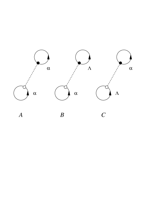
FIG. 1.: Examples of cluster diagrams contributing to the one body densities. The A diagram contributes to $\rho_{1,A}^{\alpha}(r)$, the B diagram to $\rho_{1,\Lambda}^{\alpha}(r)$ and the C diagram to $\rho_{1}^{\Lambda}(r)$. The dashed lines represent the dynamical correlations, $f^{2}_{D}(r_{ij})-1$, ($D=N$ in A and $D=\Lambda$ the rest of the cases) and the oriented lines the statistical correlations, $\rho_{0}({\bf r}_{i},{\bf r}_{j})$. A black dot associated with a point implies integration over its coordinates. The label $\alpha$ indicates the nucleon.

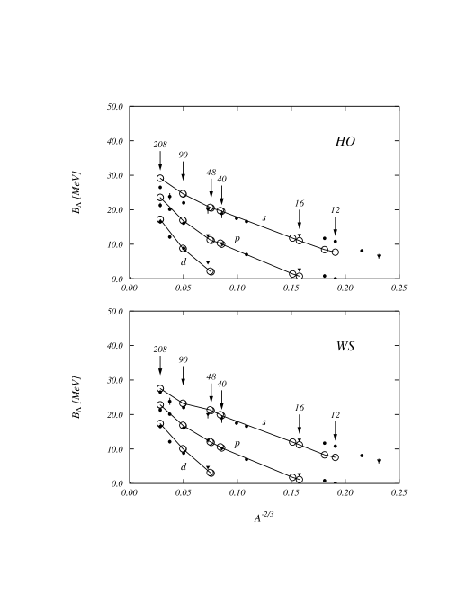
FIG. 2.: $\Lambda$ binding energies for the $1s$, $1p$ and $1d$ states, as function of $A^{-2/3}$. The white circles are the energies calculated using harmonic oscillator (upper panel) and Woods-Saxon mean field potentials (lower panel). The experimental energies are taken from Ref. [29] (dots) and [30] (triangles). The full lines connecting the theoretical values have been drawn to guide the eyes.

FIG. 3.: Proton densities for four doubly closed shell nuclei. The dotted lines are the IPM results; the dashed lines are the densities obtained by purely nucleonic FHNC calculations; the full lines are the densities obtained when a $\Lambda$ in the $s$ state is added.

FIG. 4.: Differences between proton (panel $a$) and neutron (panel $b$) densities with and without core polarization.

FIG. 5.: Differences between proton (panel $a$) and neutron (panel $b$) densities of isotopic hypernuclei with A+1 and A hadrons.

FIG. 6.: $\Lambda$ densities in $s$ and $p$ states for various hypernuclei. Dashed lines: IPM; full line: FHNC results.

REFERENCES

- [1] R. B. Wiringa, S. C. Pieper, J. Carlson, and V. R. Pandharipande, Phys. Rev. C 62, 014001 (2000).
- [2] A. Fabrocini, F. Arias de Saavedra, and G. Co’, Phys. Rev. C 61, 044302 (2000).
- [3] J. H. Heisenberg, and B. Mihaila, Phys. Rev. C 59, 1440 (1999).
- [4] A. Fabrocini, and G. Co’, Phys. Rev. C in press, arXiv:nucl-th/0012048.
- [5] M. Rayet, Ann. Phys. (N.Y.) 102, 226 (1976); Nucl. Phys. A367, 381 (1981).
- [6] D. J. Millener, C. B. Dover and A. Gal, Phys. Rev. C 38, 2700 (1988).
- [7] J. Schaffner, C. Greiner, and H. Stöcker, Phys. Rev. C 46, 332 (1992); J. Schaffner, C. B. Dover, A. Gal, C. Greiner, D. J. Millener and H. Stöcker, Ann. Phys. (N.Y.) 235, 35 (1994).
- [8] Z. Ma, J. Speth, S. Krewald, B. Chen and A. Reuber, Nucl. Phys. A608, 385 (1996).
- [9] K. Tsushima, K. Saito, and A. W. Thomas, Phys. Lett. B411, 9 (1997); D. Vretenar, W. Pölsch, G. A. Lalazissis, and P. Ring, Phys. Rev. C 57, R1060 (1998).
- [10] P. M. M. Maessen, T. A. Rijken, and J. J. de Swart, Phys. Rev. C 40, 2226 (1989).
- [11] B. Holzenkamp, K. Holinde, and J. Speth, Nucl. Phys. A500, 485 (1989).
- [12] T. A. Rijken, V. G. J. Stoks, and Y. Yamamoto, Phys. Rev. C 59, 21 (1999).
- [13] I. Vidaña, A. Polls, A. Ramos, and M. Hjorth–Jensen, Nucl. Phys. A644, 201 (1998).
- [14] J. Cugnon, A. Lejeune, and H.–J. Schulze, Phys. Rev. C 62, 064308 (2000).
- [15] Q. N. Usmani and A. R. Bodmer, Phys. Rev. C 60, 055215 (1999).
- [16] S. Rosati, in From Nuclei to Particles, Proceedings of the International School of Physics ”Enrico Fermi”, Course LXXIX, edited by A. Molinari (North Holland, Amsterdam 1982), p. 73.
- [17] I. R. Afnan, and Y. C. Tang, Phys. Rev. 175, 1337 (1968).
- [18] R. Guardiola, A. Faessler, H. Müther, and A. Polls, Nucl. Phys. A371, 79 (1981).
- [19] A.R. Bodmer, and Q.N. Usmani, Nucl. Phys. A477, 621 (1988).
- [20] A. Fabrocini, F. Arias de Saavedra, G. Co’, and P. Folgarait, Phys. Rev. C 57, 1668 (1998).
- [21] Q. N. Usmani, Nucl. Phys. A340, 397 (1980).
- [22] G. Co’, A. Fabrocini, S. Fantoni, and I. E.. Lagaris, Nucl. Phys. A549, 439 (1992).
- [23] F. Arias de Saavedra, G. Co’, A. Fabrocini, and S. Fantoni, Nucl. Phys. A605, 359 (1996).
- [24] A.A. Usmani, S. Pieper, and Q.N. Usmani, Phys. Rev. C 51, 2347 (1995).
- [25] B. Friedman, and V.R. Pandharipande, Nucl. Phys. A361, 502 (1981).
- [26] A. Fabrocini, and A. Polls, Phys. Rev. B25, 4533 (1982).
- [27] J. Boronat, F. Arias de Saavedra, E. Buendía, and A. Polls, Jour. of Low Temp. Phys. 94, 325 (1994).
- [28] G. Co’, A. Fabrocini, and S. Fantoni, Nucl. Phys. A568, 73 (1994).
- [29] T. Hasegawa et al., Phys. Rev. C 53, 293 (1996).
- [30] P. H. Pile et al., Phys. Rev. Lett. 66, 2585 (1991).
- [31] M. May et al., Phys. Rev. Lett. 78, 4343 (1997).