Elastic electron–deuteron scattering
in chiral effective field theory

Abstract

We calculate elastic electron–deuteron scattering in a chiral effective field theory approach for few–nucleon systems based on a modified Weinberg power counting. We construct the current operators and the deuteron wave function at next-to-leading (NLO) and next-to-next-to-leading (NNLO) order simultaneously within a projection formalism. The leading order comprises the impulse approximation of photons coupling to point-like nucleons with an anomalous magnetic moment. At NLO, we include renormalizations of the single nucleon operators. To this order, no unknown parameters enter. At NNLO, one four–nucleon–photon operator appears. Its strength can be determined from the deuteron magnetic moment. We obtain not only a satisfactory description of the deuteron structure functions and form factors measured in electron–deuteron scattering but also find a good convergence for these observables.

PACS: 13.40.Gp, 13.75.Cs, 12.39.Fe

Keywords: Electron–deuteron scattering, chiral effective field theory

FZJ-IKP(TH)-2001-06

,

1. A new era of nuclear physics calculations was started by Weinberg [1, 2] applying effective field theory (EFT) methods and chiral Lagrangians to systems of two and more nucleons. Although there are still some (minor) conceptual problems in the precise formulation of nuclear effective field theory, it is by now established that at very low energies, one can perform very accurate calculations using a theory of non–relativistic nucleons, whose interactions are given in terms of A-nucleon terms (A$=4,6,\ldots$) with the pions integrated out, the so–called pionless theory. Going to higher energies, the inclusion of pions becomes of prime importance and it has been shown that Weinberg’s original proposal of constructing an irreducible N–nucleon (N$=2,3,\ldots$) potential and iterating it in a Schrödinger (Lippmann-Schwinger) equation can give a precise description of nucleon–nucleon (NN) scattering as well as static and dynamic properties of three- and four-nucleon systems, see e.g. [3, 4, 5]. The more elegant formulation of Kaplan, Savage and Wise (KSW) [6], which allows for power counting on the level of the scattering amplitudes, suffers in its present formulation from the incorrect description of the tensor force, as reflected in the non–convergence of the triplet partial waves in $np$ scattering, see [7, 8]. For a much more detailed discussion of the concepts and applications of nuclear EFT, we refer to the recent reviews [9, 10]. Of course, many results found in nuclear effective field theory have previously been obtained in more conventional meson-exchange approaches [11, 12]. These, however, cannot be formulated in a truly systematic fashion and cannot be linked simply to the symmetries of QCD, as it is the case of the chiral effective field theory employed here.

In this letter, we will consider elastic electron–deuteron scattering based on a Hamiltonian approach to Weinberg’s formulation as developed in [14]. The central object will be the (unpolarized) scattering cross section, which in case of the deuteron is given in terms of two structure functions,

$$\frac{d\sigma}{d\Omega}=\left(\frac{d\sigma}{d\Omega}\right)_{\rm Mott}\,\left[A(q^{2})+B(q^{2})\tan\frac{\theta}{2}\right]~{},$$ (1)

with $q^{2}=-Q^{2}<0$ the invariant momentum transfer squared and $\theta$ is the scattering angle in the centre-of-mass frame. Furthermore, we have separated the QED (Mott) cross section. Alternatively, one can parameterize the response of the deuteron to an external vector current in terms of three form factors, $F_{C}$ (charge), $F_{M}$ (magnetic) and $F_{Q}$ (quadrupole). These latter three have been the subject of a detailed study in [15], which employed external wave functions sewed to the leading order interaction kernel. Our approach is similar, only that we construct the current operators and the wave functions simultaneously from the same Hamiltonian. Furthermore, we wish to study the interplay of nuclear and nucleon dynamics beyond the accuracy than it was done in [15]. In addition, we will be able to compare our results directly with the pioneering perturbative calculation of [17], which certainly can be considered a cornerstone in the development of nuclear effective field theory. Finally, this study is to be understood as the first step in a systematic investigation of the electromagnetic properties of light nuclei. Since much is known about the deuteron from the experimental and the theoretical side, such an investigation is clearly needed. More precisely, the deuteron is a very special nucleus due to its small binding energy, it thus can be well described by iterated one–pion–exchange and some short range physics, as it is done in conventional nuclear physics since a long time and has been perfected to high precision. The approach presented here is similar but also differs because corrections can be calculated in a controlled and systematic fashion. This becomes more important if one goes to more densely bound systems. For a more detailed discussion about the usefulness of EFT in the description of deuteron dynamics and the relation to conventional approaches, we refer to [15].

2. First, we briefly explain the central ideas underlying our calculations. One starts from an effective chiral Lagrangian of pions and nucleons, including in particular local four–nucleon interactions which describe the short range part of the nuclear force, symbolically

$${\mathcal{L}}_{\rm eff}={\mathcal{L}}_{\pi\pi}+{\mathcal{L}}_{\pi N}+{\mathcal{L}}_{NN}~{},$$ (2)

where each of the terms admits an expansion in small momenta and quark (meson) masses. To a given order, one has to include all terms consistent with chiral symmetry, parity, charge conjugation and so on. From the effective Lagrangian, one derives the two–nucleon potential. This is based on a modified Weinberg counting, which is applied to the two–nucleon potential to a certain order in small momenta and pion masses,

$$V(\vec{p},\vec{p}\,^{\prime})=\sum_{i}V^{(i)}(\vec{p},\vec{p}\,^{\prime})~{},$$ (3)

with $\vec{p},\vec{p}\,^{\prime}$ the nucleon centre-of-mass momenta and the superscript $i$ gives the (non–negative) chiral dimension. The power counting underlying this potential is based on the considerations presented in [14]. To leading order (LO), this potential is the sum of one–pion exchange (OPE) (with point-like coupling) and of two four–nucleon contact interactions without derivatives. The low–energy constants (LECs) accompanying these terms have to be determined by a fit to some data, like e.g. the two S-wave phase shifts in the low–energy region (for $np$). At next–to–leading order (NLO), one has corrections to the OPE, the leading order two–pion exchange graphs and seven dimension two four–nucleon terms with unknown LECs (for the $np$ system). Finally, at NNLO, one has further corrections in the one– and two–pion exchange graphs including dimension two pion–nucleon operators. The corresponding LECs can be determined from the chiral perturbation theory (CHPT) analysis of pion–nucleon scattering (for details, see  [4]). The existence of shallow nuclear bound states (and large scattering lengths) forces one to perform an additional nonperturbative resummation. This is done here by obtaining the bound and scattering states from the solution of a regularized Lippmann–Schwinger equation. The potential has to be understood as regularized, as dictated by the EFT approach employed here, i.e. $V({p},{p}^{\prime}\,)\to f_{R}({p})\,V({p},{p}^{\prime})\,f_{R}({p}^{\prime})$, where $f_{R}(p)$ is a regulator function chosen in harmony with the underlying symmetries. Within a certain range of cut–off values, the physics should be independent of its precise form and value. This range increases as one goes to higher orders, as demonstrated explicitly for the $np$ case in [4].

3. A powerful method to simultaneously construct wave functions and current operators was invented long time ago by Okubo and others [19, 20]. The extension to meson–exchange currents in few–nucleon systems was pioneered by Gari and Hyuga [21, 22]. As mentioned before, in [14] it was shown how this method could be extended to chiral effective Hamiltonians based on Weinberg’s power counting. The corresponding electromagnetic current, denoted by $j_{\mu}$ throughout, can now be obtained in two ways. One can either gauge the effective Hamiltonian or calculate directly the effective current from the relation

$$\langle\psi_{j}|j_{\mu}|\psi_{i}\rangle=\langle\phi_{j}|j_{\mu}^{\rm eff}|\phi_{i}\rangle~{},$$ (4)

with $|\phi\rangle$ the projected low–energy state, $|\psi\rangle=(1+A)(\eta(1+A^{\dagger}A)^{-1/2}\eta)|\phi\rangle$. Here, $\eta$ is the projector onto the Fock space with two nucleons and no pions and the operator $A$ can be obtained recursively from demanding that the wave function orthogonal to $\eta|\psi\rangle$ decouples. The effective current takes the form

$$j_{\mu}^{\rm eff}=\eta\,(1+A^{\dagger}A)^{-1/2}(1+A^{\dagger})\,j_{\mu}\,(1+A)(1+A^{\dagger}A)^{-1/2}\,\eta~{}.$$ (5)

We mention in passing that in this approach one has to include so–called wave function reorthonormalization diagrams, see e.g. [14] for the two–nucleon potential. Their contribution to the effective current is completely cancelled by the two-body recoil current (in the non-relativistic limit) [21]. Before giving the explicit form of the effective current, it is important to formulate the power counting in the presence of external electroweak fields, first worked out by Rho [18]. Denoting by $Q$ a small external momentum or a pion mass, any QCD matrix-element (in the presence of external fields) takes the form

$${\mathcal{M}}=Q^{\nu}\,f\left(\frac{Q}{\mu},g\right)$$ (6)

where $\mu$ is some regularization scale, $g$ denotes a collection of coupling (low–energy) constants and $f$ is a function of order one. The counting index is given by

$$\nu=1-2C+2L+\sum_{i}\bar{\nu}_{i}~{},\quad\bar{\nu}_{i}=d_{i}+\frac{n_{i}}{2}+e_{i}-2~{},$$ (7)

with $C$ the number of connected pieces in the diagram under consideration, $L$ the number of (pion) loops, and $\bar{\nu}_{i}$ is the vertex dimension. The latter depends on the number of derivatives/pion mass insertions $(d_{i})$, the number of nucleon fields $(n_{i}$) and the number of external fields ($e_{i})$, in our case insertions of the electromagnetic current. Chiral symmetry demands that the counting index is bounded from below, as verified by eq.(7). The terms with $C=2$ are called one–body terms in the nuclear physics language. They subsume all interactions of the photon with either the neutron or the proton (this is also called the impulse approximation). For $C=1$, obviously both nucleons are involved in the interaction, thus one talks of two–body terms (in Weinberg’s language, these terms are denoted as three–body interactions). From eq.(7), one quickly establishes that the lowest order terms are of the one–body type and have $\nu=-3$ (electric photon coupling) and $\nu=-2$ (magnetic coupling). These comprise the coupling of a photon to point–like nucleons with an anomalous magnetic moment and define the leading order. At NLO (and NNLO), we have further one–body terms, which are the usual leading one–loop (third order) chiral perturbation theory corrections to the nucleon form factors, see [23, 24, 25]. In addition, we have the leading two–body operators, the celebrated meson–exchange (seagull and pionic) currents. Using the leading order vertices as given below, these do not contribute to elastic e-d scattering (as it is well known). Also, based on this counting, one has no local four–nucleon–photon interactions at NLO. The first correction, which is not of one–body nature, does appear at NNLO, it is the magnetic four–nucleon–photon interaction of [17]. At that order, one has also one–body corrections proportional to the magnetic radii of the proton and the neutron. We should point out one subtlety with the power counting here. In terms of the wave functions, the current operators at NLO and NNLO are only sensitive to the NLO wave functions, which can be simply understood from the fact that gauging the corresponding operators in the potential does lead to even higher orders in the current. Therefore, the results for the electric and the quadrupole form factor at NLO and NNLO will coincide, and we denote them as (N)NLO. Formally, one could therefore subsume what we call NLO and NNLO here simply as NLO, similar to the two orders making up the LO (impulse) contribution. Since this has not be done in the existing literature, see e.g. ref. [16], we refrain from doing so too.

We now discuss the effective interaction Hamiltonians including the photon field, expressed in terms of the gauge potential $A_{\mu}$ and the field strength tensor $F_{\mu\nu}$. From these, the effective current follows. Gauging the free and the interaction Hamiltonians, ${\mathcal{H}}_{0}$ and ${\mathcal{H}}_{\rm int}$, respectively, gives (we only show the terms that involve the photon field, all other terms to the order we are working are given e.g. in [14]),

$${\mathcal{H}}_{0}^{\rm em} = -N^{\dagger}\left(-i\frac{\hat{e}_{N}}{m_{N}}{A}_{i}\,{\nabla}^{i}+\hat{e}_{N}A^{0}+\frac{e\,\kappa_{s}}{2m_{N}}\,\sigma_{i}\,\epsilon^{ijk}\,F_{ik}+\ldots\right)N$$ (8)

$$\quad+\left(\left(\frac{\partial}{\partial t}\pi_{a}\right)i\hat{e}_{\pi}A^{0}\pi^{a}\right)-\left(\left(\nabla_{i}\pi_{a}\right)i\hat{e}_{\pi}A^{i}\pi^{a}\right)~{},$$

$${\mathcal{H}}_{\rm int}^{\rm em} = \frac{g_{A}}{2F_{\pi}}\,N^{\dagger}{\tau}_{a}\,\sigma_{i}(-i\hat{e}_{\pi}A^{i})\,{\pi}^{a}\,N-eL_{2}\,(N^{\dagger}\,\sigma_{i}\,\epsilon^{ijk}\,F_{ik}\,N)(N^{\dagger}N)~{},$$ (9)

with $\hat{e}_{N}$ and $\hat{e}_{\pi}$ the nucleon and pion charge matrix, respectively, and $m_{N}$ is the nucleon mass. We omit terms of higher order in the electromagnetic coupling since they are not relevant here. Throughout, we work in the Coulomb gauge $\vec{\nabla}\cdot\vec{A}=0$. For the gauged free nucleon Hamiltonian, we have only given the leading order (dimension one) electric coupling and the (dimension two) magnetic one, with $\kappa_{s}$ the isoscalar anomalous magnetic moment of the nucleon, $(\kappa_{p}+\kappa_{n})/2=\kappa_{s}$. These two interactions lead to the terms with $\nu=-3$ and $-2$ as discussed before. The dimension three terms contributing to the one–body currents at $\nu=-1$ can be found in [24]. The pion–photon–nucleon interaction in eq.(9) is nothing but the celebrated Kroll-Ruderman term, with $g_{A}$ the axial vector coupling measured in neutron $\beta$–decay and $F_{\pi}$ the weak pion decay constant. As noted before, employing these Hamiltonians, the leading exchange currents are proportional to $\vec{\tau}_{1}\times\vec{\tau}_{2}$ (where $\vec{\tau}_{i}$ is the isospin operator of nucleon $i$) and thus vanish for isoscalar transitions as it is the case for e-d scattering. The leading isoscalar exchange current appears only at N³LO, because the only possible NNLO term would consist of a dimension two correction to the Kroll-Ruderman vertex. This operator has the structure $\sigma_{i}\epsilon^{i}\,v_{\mu}q^{\mu}\,(\tau^{a}+\delta^{a3})$ (see app. A of [26]) and thus generates only an isovector operator. At N³LO, we have contributions from two–pion–exchange diagrams with one $\gamma\pi\pi\bar{N}N$–vertex (football and triangle graphs) together with dimension three corrections to the pion-nucleon-photon vertex. The last term in eq.(9), first considered in [17], is a magnetic photon four–nucleon contact interaction, its strength can not be determined from np scattering but can be obtained from a fit to the deuteron magnetic moment. We note that there is also a NNLO single nucleon correction due to the magnetic radius. We stress that such power counting arguments have already been given in [15].

4. We now turn to the response of the deuteron to an external electromagnetic field. Consider a deuteron state with four–momentum ${p}_{\mu}$ and polarization vector $\vec{\epsilon}\,^{\mu}$, subject to the condition $p_{\mu}\vec{\epsilon}\,^{\mu}=0$. In the deuteron rest frame, one conventionally selects $\epsilon^{\mu}_{i}=\delta_{i}^{\mu}$ and the corresponding deuteron states are denoted by $|\vec{p},i\rangle$. In terms of these and to leading order in the non-relativistic expansion, the matrix element of the electromagnetic current is given in terms of the charge, magnetic and quadrupole form factors,

$$\langle\vec{p}\,^{\prime},i\,|\,j_{0}\,|\,\vec{p},j\rangle = e\,\left[F_{C}(Q^{2})\,\delta_{ij}+\frac{1}{2m_{d}^{2}}F_{Q}(Q^{2})\left(\vec{q}_{i}\vec{q}_{j}-\frac{1}{3}\vec{q}\,^{2}\delta_{ij}\right)\right]~{},$$

$$\langle\vec{p}\,^{\prime},i\,|\,j_{k}\,|\,\vec{p},j\rangle = \frac{e}{2m_{d}}\,\left[F_{C}(Q^{2})\,\delta_{ij}(\vec{p}+\vec{p}\,^{\prime})_{k}+F_{M}(Q^{2})(\delta_{jk}\vec{q}_{i}-\delta_{ik}\vec{q}_{j})\right.$$ (10)

$$\qquad\quad+\left.\frac{1}{2m_{d}^{2}}F_{Q}(Q^{2})\left(\vec{q}_{i}\vec{q}_{j}-\frac{1}{3}\vec{q}\,^{2}\delta_{ij}\right)(\vec{p}+\vec{p}\,^{\prime})_{k}\right]~{},$$

with $\vec{q}=\vec{p}\,^{\prime}-\vec{p}$, $Q=|\vec{q}\,|$ and $m_{d}$ is the deuteron mass. These form factors are dimensionless and normalized to the charge, the magnetic moment, $\mu_{d}$, and the quadrupole moment, $Q_{d}$, of the deuteron, i.e. $F_{C}(0)=1$, $(e/2m_{d})F_{M}(0)=\mu_{d}$ and $(1/m_{d}^{2})F_{Q}(0)=Q_{d}$, with $\mu_{d}=0.85741\,(e/2m_{N})$ and $Q_{d}=0.2859\,$fm². The structure functions $A(Q^{2})$ and $B(Q^{2})$ defined in eq.(1) are given in terms of these form factors via

$$A = F_{C}^{2}+\frac{2}{3}\eta F_{M}^{2}+\frac{8}{9}\eta^{2}F_{Q}^{2}~{},$$

$$B = \frac{4}{3}\eta(1+\eta)F_{M}^{2}~{}.$$ (11)

Here, $\eta=Q^{2}/4m_{d}^{2}$. To disentangle these three form factors, one measurement involving polarization is necessary. The analyzing power $t_{20}$ has become the observable of choice to do that. Since it depends on $Q^{2}$ and the scattering angle $\theta$, one also uses the quantity $\tilde{t}_{20}$,

$$\tilde{t}_{20}=-\frac{\frac{8}{3}\eta F_{C}(Q^{2})F_{Q}(Q^{2})+\frac{8}{9}\eta^{2}F_{Q}^{2}(Q^{2})}{\sqrt{2}\left[F_{C}^{2}(Q^{2})+\frac{8}{9}\eta^{2}F_{Q}^{2}(Q^{2})\right]}~{},$$ (12)

which only depends on the momentum transfer squared and is independent of the magnetic form factor. Note, however, that $\tilde{t}_{20}$ is not directly measurable (for a detailed discussion, we refer to the recent review [27]).

5. We first consider the structure functions $A$ and $B$ which can be obtained directly from elastic e-d scattering. Since from the study of the nucleon form factors in heavy baryon chiral perturbation theory it is known that the third order result for the isoscalar form factor starts to deviate from the data at $Q^{2}\simeq 0.2\,$GeV², we will limit our range of $Q$ from 0 to 400$\ldots$500 MeV. We work out the matrix elements from eqs.(Elastic electron–deuteron scattering in chiral effective field theory) and construct the structure functions by use of eqs.(Elastic electron–deuteron scattering in chiral effective field theory) without any approximation. This is different from [17], where the kinematical factors like e.g. $\eta$ where also included in the power counting and thus in their case there can be no contribution from $F_{Q}(Q^{2})$ to $A(Q^{2})$ at NLO. Throughout, we work with an exponential regulator $f_{R}(p)=\exp(-p^{4}/\Lambda^{4})$ with a cut–off $\Lambda=600\,$MeV (similar to what was done in the simultaneous fit to $np$ and $pp$ scattering phases, see [28]). None of the results presented here depends notably on the cut–off within its allowed bounds. For completeness, we give the corresponding LECs. At LO, we have $\tilde{C}_{3S1}=0.0427\cdot 10^{4}\,$GeV^-2 and at NLO, we get $\tilde{C}_{3S1}=-0.0368\cdot 10^{4}\,$GeV^-2, ${C}_{3S1}=0.186\cdot 10^{4}\,$GeV^-4 and ${C}_{3S1-3D1}=-0.190\cdot 10^{4}\,$GeV^-4. These numbers are in good agreement with what has been found before using such type of regulator, see e.g. ref. [29].

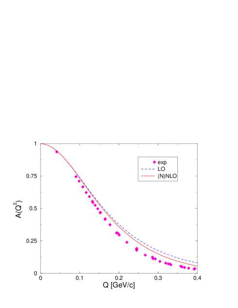
Figure 1: The structure function A($Q^{2}$). The dashed and the solid line give the LO, the (N)NLO result, respectively, and the data are from [30], [31]. As explained in the text, the NLO and NNLO results for $A(Q^{2})$ can not be distinguished on the scale of the figure.

Let us discuss $A(Q^{2})$ as given in fig. 1. Note that we plot the structure function versus $Q\equiv\sqrt{Q^{2}}$ (not versus $Q^{2}$) to facilitate the comparison with ref. [17]. The leading order curve already gives a fair description of the data, the NLO and NNLO result is visibly improved but still above the data. Note that the difference between NLO and NNLO stems from a Foldy–type contribution proportional to the magnetic radius, which is very small, and an induced contribution from the magnetic photon–four–nucleon interaction. Both of these are small and further suppressed by a factor of $\eta$, so that the difference between the two curves can not be seen on the scale of fig. 1. Since there is no exchange current contribution, the improvement going from LO to NLO is due to the single nucleon radius terms which appear at this order. This can be seen by considering the LO wave function together with the NLO current operators. At yet higher orders, however, there should be some further improvement due to the wave functions as shown in [15]. One should consider such a sensitivity to single nucleon observables not as an unwanted complication but rather conclude that indeed isoscalar quantities (alas neutron properties) can be inferred from nuclear targets with some precision. We consider this interplay of chiral nucleon dynamics and nuclear EFT as one of the important ingredients in the whole approach. Note further that our (N)NLO result is similar to the one of [17]. It should also be noted that for the range of momentum transfer considered here, the NLO corrections are sizeably smaller than in the KSW calculation, pointing towards a better convergence.

Next, we turn our attention to $B(Q^{2})$, which is essentially the response to the magnetic photon, see fig. 2. Again, the LO result is visibly better than the one obtained in [17], whereas the NLO curves are comparable. However, in contrast to the work of [17], our prediction for $B(Q^{2})$ is parameter–free, whereas the one in the KSW scheme has one free parameter from the four–nucleon–photon interaction (due to the different counting). Also, the NLO correction is fairly small for the momentum range considered here, indicating convergence. At NNLO, we have to pin down the LEC $L_{2}$ of the magnetic photon four–nucleon interaction, which is done by fitting the magnetic moment of the deuteron. The resulting curve for $B(Q^{2})$ is further improved, see fig. 2.

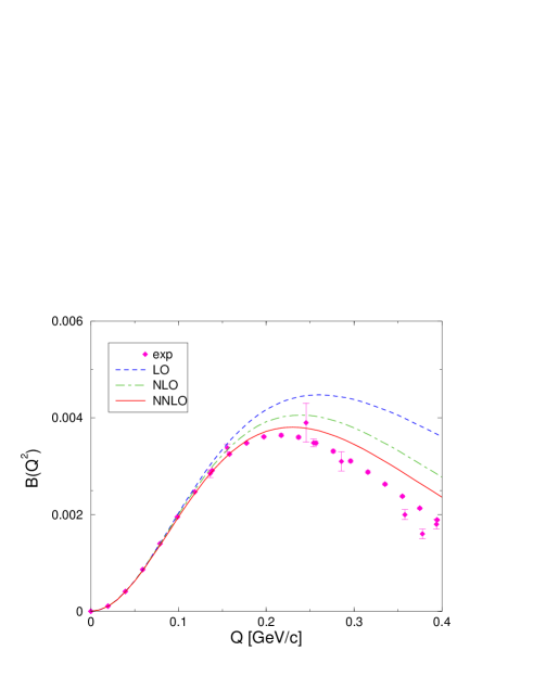
Figure 2: The structure function B($Q^{2}$). The dashed, the dot-dashed and the solid line give the LO, the NLO and the NNLO result, respectively. The new data are from the compilation of Sick [32] (filled diamonds) and the older data (open circles) are from [33], [34], [35].

Next, we discuss the charge, magnetic and quadrupole form factors. The corresponding normalizations (static properties) are collected in table 1 for LO and NLO. The only difference at NNLO is the magnetic moment, which is exactly reproduced (since it is used as input to fix $L_{2}$). The corresponding value for the the LEC $L_{2}$ is $L_{2}=2.68\cdot 10^{-2}\,$GeV^-2, which is rather small. This can be traced back to the fact that the NLO result for $\mu_{d}$ is already within 1% of the empirical value. Note that in contrast to what was done in ref.[4], we have fine tuned the LECs in the deuteron channel to reproduce the binding energy to four digits. The only difference at NNLO to NLO is the magnetic moment, therefore the NNLO numbers are not given. Notice that with the fine tuned binding energy, the prediction for the quadrupole moment is visibly improved as compared to ref. [4] and closer to the data than in all modern high–precision potentials.

Table 1: Static properties at LO and NLO. Here, $E_{d}$, $\mu_{d}$ and $Q_{d}$ denote the deuteron binding energy, its magnetic and its quadrupole moment.

	LO	NLO	Exp.
$|E_{d}|$ [MeV]	2.224	2.224	2.22456612(12)
$\mu_{d}$ [$\mu_{N}$]	0.828	0.852	0.8574382284(94)
$Q_{d}$ [fm2]	0.265	0.276	0.2859(3)

In all cases, the NLO/NNLO corrections are small and one finds a decent description of the three form factors, see fig. 3. The largest discrepancies at higher momentum transfers are found in the charge form factor, as reflected in the results for $A(Q^{2})$ shown above. Similar results have been obtained in [15], however, a direct comparison with data was not given in that paper.

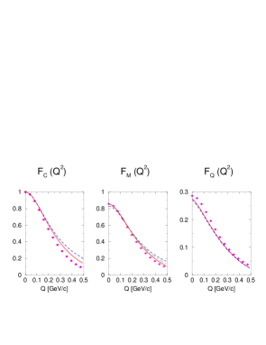
Figure 3: Electric, $F_{C}(Q^{2}$), magnetic, $F_{M}(Q^{2})$, and quadrupole, $F_{Q}(Q^{2})$, form factors of the deuteron, in order. The dashed, the dot-dashed and the solid lines give the LO, the NLO (only shown for $F_{M}$) and the NNLO results, in order, and the data are from the analysis of Sick [32]. As explained in the text, NLO and NNLO results coincide for the electric and the quadrupole form factor.

From the electric and the quadrupole form factor, we can construct $\tilde{t}_{20}$, as shown in fig. 4. Again, the deviations of our LO and (N)NLO predictions for $F_{C}(Q^{2})$ from the data are responsible for the too small magnitude of $\tilde{t}_{20}$ at $Q\simeq 0.4\,$GeV.

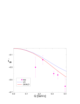
Figure 4: Analyzing power $\tilde{t}_{20}$ at LO (dashed) and (N)NLO (solid line). The data are from the recent compilation [36].

6. We have analyzed electron–deuteron scattering in the framework of a chiral effective field theory for few–nucleon systems at next–to–leading and next–to–next–to–leading order. At NLO, no meson–exchange currents or four–nucleon–photon operators contribute. At NNLO, only one magnetic photon–four–nucleon operator appears, the corresponding coupling constant can be determined from a fit to the deuteron magnetic moment. As stressed, the NLO and NNLO predictions for the electric and the quadrupole form factors coincide at NLO and NNLO because one is not yet sensitive to the NNLO wave function corrections. In particular, we have discussed the interplay between the single nucleon dynamics as encoded in the nucleon form factors and the nuclear dynamics. As already stressed in [15], the accuracy of the description of the nucleon form factors limits the applicability of the effective field theory approach to the deuteron structure to momentum transfer of about $Q\simeq 0.4$ GeV. Thus an improved description of these single nucleon observables has to be obtained to extend these considerations consistently to higher photon virtualities. For a step in this directions, see [25]. We stress again that we consider it important to consistently describe the single as well as the few–nucleon sector. The results presented here extend the ones of [15] to the first non–trivial order for the single nucleon form factors, i.e. are sensitive to the structure of the nucleon. Obviously, as next steps one has to consider N³LO corrections to the process discussed here (since only at that order sufficiently many additional contributions appear, like e.g. meson–exchange currents) as well as electron scattering of three- and four–body systems, using the wave functions of [5].

Acknowledgements

We are grateful to Manfred Gari for a useful discussion, Ingo Sick for providing us with the e-d scattering data and his analysis of these and Rocco Schiavilla for supplying his data base. We thank Daniel Phillips for some clarifying remarks on the work presented in [15] and Bastian Kubis for comments and a careful reading of the manuscript.

References

- [1] S. Weinberg, Phys. Lett. B251 (1990) 288.
- [2] S. Weinberg, Nucl. Phys. B363 (1991) 3.
- [3] C. Ordonez, L. Ray and U. van Kolck, Phys. Rev. C53 (1996) 2086.
- [4] E. Epelbaum, W. Glöckle and Ulf-G. Meißner, Nucl. Phys. A671 (2000) 295.
- [5] E. Epelbaum et al., Phys. Rev. Lett. 86 (2001) 4787.
- [6] D.B. Kaplan, M.J. Savage and M.B. Wise, Nucl. Phys. B534 (1998) 329.
- [7] T. Mehen, S. Fleming and I.W. Stewart, Nucl. Phys. A677 (2000) 313.
- [8] G. Rupak and N. Shoresh, nucl-th/9906077.
- [9] U. van Kolck, Prog. Nucl. Part. Phys. 43 (1999) 409.
- [10] S.R. Beane et al., in Boris Ioffe Festschrift - ”At the Frontier of Particle Physics – Handbook of QCD”, Vol. 1, M. Shifman (ed.) (World Scientific, Singapore, 2001), nucl-th/0008064.
- [11] D.O. Riska, Phys. Rep. 181 (1989) 207.
- [12] J. Carlson and R. Schiavilla, Rev. Mod. Phys. 70 (1998) 743.
- [13] Ulf-G. Meißner and M.F. Gari, Phys. Lett. 125B (1983) 364.
- [14] E. Epelbaoum, W. Glöckle and Ulf-G. Meißner, Nucl. Phys. A637 (1998) 107.
- [15] D.R. Philipps and T. Cohen, Nucl. Phys. A668 (2000) 45.
- [16] T.-S. Park, D.-P. Min and M. Rho, Nucl. Phys. A595 (1996) 515.
- [17] D.B. Kaplan, M.J. Savage and M.B. Wise, Phys. Rev. C59 (1999) 617.
- [18] M. Rho, Phys. Rev. Lett. 66 (1991) 1275.
- [19] S. Okubo, Prog. Theor. Phys. 12 (1954) 603.
- [20] N. Fukuda, K. Sawada and M. Taketani, Prog. Theor. Phys. 12 (1954) 156.
- [21] M.F. Gari and H. Hyuga, Z. Phys. A277 (1976) 291.
- [22] M.F. Gari and H. Hyuga, Nucl. Phys. A278 (1977) 372.
- [23] V. Bernard, N. Kaiser, J. Kambor and Ulf-G. Meißner, Nucl. Phys. B388 (1992) 315.
- [24] V. Bernard, H.W. Fearing, T.R. Hemmert and Ulf-G. Meißner, Nucl. Phys. A635 (1998) 121; (E) Nucl. Phys. A642 (1998) 563.
- [25] B. Kubis and Ulf-G. Meißner, Nucl. Phys. A679 (2001) 698.
- [26] V. Bernard, N. Kaiser and Ulf-G. Meißner, Int. J. Mod. Phys. E4 (1995) 193.
- [27] M. Garçon and J.W. Van Orden, nucl-th/0102049.
- [28] M. Walzl, Ulf-G. Meißner and E. Epelbaum, nucl-th/0010019, Nucl. Phys. A (2001) in press.
- [29] E. Epelbaum, doctoral thesis, published in Berichte des Forschungszentrum Jülich, No. 3803 (2000).
- [30] G.G. Simon, Ch. Schmitt and V.H. Walther, Nucl. Phys. A364 (1981) 285.
- [31] S. Platchkov et al., Nucl. Phys. A510 (1990) 740.
- [32] I. Sick, private communication.
- [33] B. Grosstete, D. Drickey and P. Lehmann, Phys. Rev. 141 (1966) 1425.
- [34] D. Benaksas, D. Drickey and D. Frerejacque, Phys. Rev. 148 (1966) 1327.
- [35] D. Ganichot, B. Grosstete and D.B. Isabelle, Nucl. Phys. A178 (1972) 545.
- [36] D. Abbott et al., Eur. Phys. J. A7 (2000) 421.