Abstract

The purpose of the present article is to call attention to some realistic quasiparticle-based description of the quark/gluon matter and its consistent implementation in thermodynamics. A simple and transparent representation of the thermodynamical consistency conditions is given. This representation allows one to review critically and systemize available phenomenological approaches to the deconfinement problem with respect to their thermodynamical consistency. A particular attention is paid to the development of a method for treating the string screening in the dense matter of unbound color charges. The proposed method yields an integrable effective pair potential which can be incorporated into the mean-field picture. The results of its application are in reasonable agreement with lattice data on the QCD thermodynamics.

PACS numbers: 24.85.+p, 12.38.Aw, 12.38.Mh, 21.65.+f, 64.60.-i

1 Introduction

With the advent of RHIC and LHC, there is a growing need for a deeper understanding of various properties of the QCD matter at high temperature and finite density. At the moment, we are still far from a satisfactory level in this respect, even for equilibrium properties of quark–gluon plasma. Indeed, though such a system can in principle be approximated as a gas of quarks and gluons, a fully perturbative calculation with these degrees of freedom does in practice not work well at any reasonable temperature since the perturbative series are badly converged due to infrared-sensitive contributions. On the other hand, the QCD lattice calculation, the only systematic fully nonperturbative method available, is restricted in the presence of light dynamical quarks, and even more so in the presence of a finite baryon density (see [1] where the current state of art is summarized). Therefore, various phenomenological, QCD-motivated models are called up for describing the thermodynamics of highly excited nuclear matter and its Equation of State (EoS).

General arguments from QCD and lattice data tell that a kind of string is developed between quarks and antiquarks at large distance and it is natural to identify such $q\bar{q}$ system with conventional mesons. Treating quark and gluon propagation in the confining QCD vacuum within non-Abelian SU(3) gauge theory, the string dynamics was successfully applied to conventional mesons, hybrids, glueballs and gluelamps. However, if such a string is surrounded by unbound quarks and gluons, the $q\bar{q}$ system can be excited not only in color-singlet states, but also in color-octet states or even dissociate into constituent elements. The latter will signal, in general, on the deconfinement phase transition. These phase transformations are intimately related to the change of string properties (in particular, color charges of quarks are screened in quark-gluon environment): string behavior becomes medium dependent.

By now, there is a number of simplified models for describing static hadron properties as well as a highly excited, deconfined state of quark matter, the quark-gluon plasma (QGP). A common feature of these models is that they all are based on a quasiparticle picture, considering isolated particle-like degrees of freedom and assuming that these quasiparticles are moving in a background mean field. Two- and many-particle correlations are included in the mean-field contributions and in the modification of the one-particle spectra. Well-known examples are the original bag model and its later versions [2, 3, 4], phenomenological approaches with temperature-dependent bag constant [5, 6], string-motivated density-dependent corrections to an ideal (massive or massless) quark matter equation of state, the very consideration of hadrons as composite objects in QCD, excluded volume corrections [7, 8], and finally mixed phase [9] and chemical mixture [10, 11] models dealing with the transition between quark matter and hadron matter in a phenomenological way.

The present paper concerns the quasiparticle description of the QCD thermodynamics with the particular emphasis on the mean-field treatment of in-medium strings. The paper is organized as follows. In Sec.II we consider the thermodynamical consistency of the quasiparticle description in general. Any phenomenological approach, involving a quasiparticle interaction, usually operates with a Hamiltonian which may depend on thermodynamical characteristics of the surrounding matter, like the temperature $T$ and density $n$. As is known for a long time (see, for details, [12, 13]), there exist certain restrictions to the dependence of such a Hamiltonian on the thermodynamic variables.In this section a transparent and useful representation of these restrictions is derived [see Eqs.(21) and (22)] which directly involves the quasiparticle spectra. The obtained representation of thermodynamical consistency allows us to get an instructive relation between a number of modern approaches, dealing with the deconfinement problem in the framework of a quasiparticle picture, as exemplified in the end of Sec.II. The QCD-motivated interactions, in particular string-like interactions [14], are under investigation in Sec.III. A comprehensive model of string formation in the dense matter of unbound color charges is developed, which supports the choice of the mean field proportional to an inverse power of the color-charge density, as proposed in the papers [9, 12, 15, 16, 17]. This quasiparticle scheme is applied in Sec.IV for thermodynamics of the deconfined QCD phase. The case when the system is in thermal equilibrium but not in chemical one is also considered. The results are summarized in the concluding Sec.V.

2 Quasiparticle Hamiltonian

In order to obtain an effective quasiparticle description of a medium made of unbound colour charges, one should operate with screened long-range potentials. A natural way to introduce the screening in quark matter is based on using the probability density $P(r)$ to form a string of the length $r$. It is worth noting that this investigating scheme has much in common with another one which deals with the probability density that the nearest neighbour occurs at a distance $r$ [16]. Both approaches involve thermodynamical variables, which lead to a screened pair potential depending on thermodynamical quantities. Due to such effects the quasiparticle Hamiltonian becomes density and temperature dependent, which in turn leads to a modification of a thermodynamical potential (e.g. the Gibbs free energy). Eventually a nonideal EoS emerges.

2.1 General structure of Hamiltonian

We start with the general quasiparticle Hamiltonian

$$\hat{H}=\sum_{i}\sum_{k}\epsilon_{ki}(T,n)\ a^{{\dagger}}_{{\bf k}i}\ a_{{\bf k}i}+V\Phi(T,n).$$ (1)

Here $a^{{\dagger}}_{{\bf k}i}$ and $a_{{\bf k}i}$ are the usual creation and annihilation operators for quasiparticles of the $i$-th sort with momentum $k$. They also may depend on other internal degrees of freedom like spin, color, isospin, etc. The volume $V$ is constant and large enough (infinite in the thermodynamical limit). So in this limit, the summation over quantum states labeled by $k$ can be replaced by a phase space integral (including the internal degeneracy factor $d_{i}$):

$$\sum_{k}\rightarrow V\,d_{i}\,\int\!\frac{d^{3}k}{(2\pi)^{3}}.$$ (2)

In general, the one-particle energy $\epsilon_{ki}(T,n)$ and the background field contribution $\Phi(T,n)$ to the energy density, both depend on the temperature $T$ and the set of particle densities $n\equiv\{n_{1},n_{2},\ldots\}$. Notice that the quantity $V\Phi(T,n)$ is nothing else but the energy of the quasiparticle vacuum. Generally speaking, it differs from the vacuum of primordial particles, which leads to the $c$-number term appearing in Eq. (1). In the present paper we consider the situation when, similarly to the case of the Hartree-Fock quasiparticles, the expectation value of the quasiparticle number operator $\hat{N}_{i}=\sum_{k}\,a^{{\dagger}}_{{\bf k}i}a_{{\bf k}i}$ equals to the number of primordial particles $N_{i}=n_{i}V$. This implies that we deal with the picture of quasiparticles interacting and, thus, correlating with each other. In turn, the expectation value of the Hamiltonian has to be equal to the mean energy of the system under consideration. This leads to the following relations:

$$<\hat{H}> = E=V\sum_{i}d_{i}\int\frac{d^{3}k}{(3\pi)^{3}}\;\epsilon_{ki}\ \nu_{ki}+V\Phi,$$ (3)

$$<\hat{N}_{i}> = N_{i}=Vd_{i}\int\frac{d^{3}k}{(2\pi)^{3}}\;\nu_{ki},$$ (4)

with the occupation numbers $\nu_{ki}=\langle a^{{\dagger}}_{{\bf k}i}a_{{\bf k}i}\rangle$. There is another way of calculating the mean energy $E=V\varepsilon(T,n)$ and mean multiplicity $N_{i}=Vn_{i}$ which proceeds from a thermodynamical potential rather than from Eqs. (3) and (4). For density- and temperature-dependent Hamiltonians these different ways may lead to different results (see, for example [9, 12]). Hence, in what concerns the dependence on $n$ and $T$, the quasiparticle Hamiltonian will have a correct structure only if the thermodynamical consistency requirements (3) and (4) are satisfied when starting with either the Hamiltonian or the thermodynamical potential.

2.2 Chemical potentials

Using temperature $T$ and number densities $n_{i}=N_{i}/V$ as basic descriptive variables, the thermodynamical behavior and the appropriate EoS can be derived from the corresponding thermodynamical potential, the free energy $F(V,N,T)$:

$$F\equiv Vf=T\sum_{i}\xi_{i}\ d_{i}\int\frac{d^{3}k}{(2\pi)^{3}}\,\ln\,\left(1-\xi_{i}\ e^{-z_{ki}}\right)+V\sum_{i}\mu_{i}\ n_{i}+V\Phi.$$ (5)

Here $\xi_{i}=\pm 1$ is determined by the quasiparticle statistics, $\mu_{i}$ stands for the chemical potential of the quasiparticles of the $i$-th sort, and $z_{ki}$ is defined by

$$z_{ki}=\frac{\epsilon_{ki}-\mu_{ki}}{T}.$$ (6)

The simplest way of calculating the free energy implies the use of the grand canonical ensemble when particle numbers are known only in average and chemical potentials, $\mu_{i},$ are introduced instead of $N_{i}$ as descriptive thermodynamical variables. To calculate the partition function in this case, the quasiparticle Hamiltonian (1) should be modified to

$$\hat{H}^{\prime}=\hat{H}-\sum_{i}\mu_{i}\hat{N}_{i},$$ (7)

where $\hat{H}$ is defined by Eq. (1). We recall that the physical meaning of $\mu_{i}$ is the energy loss by removing a quasiparticle of the $i$-th species while the total entropy and volume of the system are kept constant. This chemical potential a priori has nothing to do with the fact whether this particle really carries a conserved charge or not. However, there are Lagrange multipliers associated to the conservation laws of such charges like the baryon number, strangeness or electric charge. In order to elucidate the difference between chemical potentials in general and those associated to the conserved charges, let us consider a particle mixture of many sorts whose abundance is known only in average. The mixture components (not necessarily all of them) carry some conserved charges. The conservation of these charges is controlled by the appropriate chemical potential. We denote such a charge of type $b$ carried by a particle belonging to the $i$-th component of the mixture as $q_{bi}$. Then for conserved quantities we have

$$Q_{b}=\sum_{i}q_{bi}N_{i}.$$ (8)

Usually there are more components than the number of conserved charges. In particular, it is the case for quark-gluon matter, to which we pay special interest in the present paper. Besides the case of a one-component system, the set of Eq. (8) is insufficient for calculating all mean numbers for the mixture components. Therefore, we need some additional requirements which would allow us to determine the particle numbers $N_{i}$ by making use of Eq. (8). The chemical equilibrium is usually assumed and then these additional requirements are given by

$$\mu_{i}^{{\rm eq}}=\sum_{b}q_{bi}\mu_{b},$$ (9)

where $\mu_{b}$ stands for the chemical potential associated to the charge sort $b$. In the general case, when the system is out of chemical equilibrium and the component concentrations become time-dependent, the chemical potential can be split into two parts,

$$\ \mu_{i}=\sum_{b}q_{ib}\mu_{b}\,+\,\widetilde{\mu}_{i}\,,$$ (10)

and Eq. (7) is reduced to

$$\hat{H}^{\prime}=\hat{H}-\sum_{b}\mu_{b}\hat{Q}_{b}-\sum_{i}\widetilde{\mu}_{i}\hat{N}_{i}.$$ (11)

The quantities $\widetilde{\mu}_{i}$ describe the deviation from chemical equilibrium in the thermally equilibrated system. They are exactly zero in the chemical equilibrium limit, resulting in the familiar relation

$$\hat{H}_{eq}^{\prime}=\hat{H}-\sum_{b}\mu_{b}\hat{Q}_{b}.$$ (12)

Below we shall investigate consistency of the quasiparticle picture in thermodynamical treatment including the possibility of deviations from chemical equilibrium in a mixture.

2.3 Thermodynamical consistency

As mentioned above, any approach starting with a thermodynamical potential appears to be thermodynamically consistent. In other words, if all the quantities of interest can be calculated only through the derivatives of this thermodynamical potential, one is prevented from encountering thermodynamical inconsistency. Problems arise, however, when calculation can proceed not only from the constructed thermodynamical potential but also from a more fundamental level, some quasiparticle Hamiltonian at a given temperature and/or density. In the last case the result may depend on the calculation method unless the quantities $\epsilon_{ki}(T,n)$ and $\Phi(T,n)$ obey relations derived in accordance with the consistency requirements (3) and (4). These relations are below called as conditions of thermodynamical consistency.

To elaborate on these conditions, let us consider a system with the Hamiltonian defined by Eqs. (1) and (7). If the abundance of all mixture components is known only in average, the proper thermodynamical potential has the form

$$\Omega=E-TS-\sum_{i}\mu_{i}\ N_{i},$$ (13)

with $S$ being the total entropy. The grand-canonical partition function corresponding to $H^{\prime}$ can readily be calculated

$$Z\!=\!{\rm tr}\,\!(e^{-\hat{H}^{\prime}/T})\!=\!\left(\prod_{k,i}\sum_{n_{ki}}\!\!e^{-z_{ki}n_{ki}}\right)\ e^{-\Phi V/T}=e^{-\Omega/T}.$$ (14)

Recall that in the Fermi-gas case the integer quantity $n_{ki}$ equals either $0$ or $1$, while in the Bose one it runs from $0$ to $\infty$. Hence, from Eq. (14) it follows that

$$\frac{\Omega}{V}=\,T\sum_{i}d_{i}\xi_{i}\int\frac{d^{3}k}{(2\pi)^{3}}\ln\left(1-\xi_{i}e^{-z_{ki}}\right)+\Phi.$$ (15)

Note that Eq. (15) covers Eq. (5) with the definition $F=E-T\,S$. It is well-known that for the Hamiltonian $H^{\prime}$ the average quasiparticle occupation number $\nu_{ki}$ is

$$\nu_{ki}=\langle n_{ki}\rangle=\frac{1}{e^{z_{ki}}-\xi_{i}},$$ (16)

which together with Eq. (15) leads to

$$\frac{\Omega}{V}=\Phi\,-\,T\sum_{i}d_{i}\xi_{i}\int\frac{d^{3}k}{(2\pi)^{3}}\ \ln\left(1+\xi_{i}\ \nu_{ki}\right).$$ (17)

The total differential of the thermodynamical potential $\Omega$ is given by

$$d\Omega = dV\left(\Phi-T\sum_{i}d_{i}\xi_{i}\int\frac{d^{3}k}{(2\pi)^{3}}\ \ln\left(1+\xi_{i}\ \nu_{ki}\right)\right)$$ (18)

$$- VT\sum_{i}d_{i}\xi_{i}\int\frac{d^{3}k}{(2\pi)^{3}}\left(\frac{dT}{T}\ln\left(1+\xi_{i}\ \nu_{ki}\right)+\frac{\xi_{i}\ d\nu_{ki}}{1+\xi_{i}\ \nu_{ki}}\right)+Vd\Phi.$$

Since in the grand-canonical ensemble the quasiparticle densities $n_{i}$ and average occupation numbers $\nu_{ki}$ are functions of the temperature $T$ and chemical potentials $\mu_{i}$, all the differentials can be expanded in terms of $dT$, $dV$ and $d\mu_{i}$. In particular, we have

$$d\nu_{ki} = -\nu_{ki}\ (1+\xi_{i}\ \nu_{ki})\ d\left(\frac{\epsilon_{ki}-\mu_{i}}{T}\right),$$

$$d\epsilon_{ki} = \frac{\partial\epsilon_{ki}}{\partial\mu_{j}}\ d\mu_{j}+\frac{\partial\epsilon_{ki}}{\partial T}\ dT,$$

$$d\Phi = \frac{\partial\Phi}{\partial\mu_{j}}\ d\mu_{j}+\frac{\partial\Phi}{\partial T}\ dT.$$

Inserting this relations into Eq. (18) and comparing then the derived result with the general formula

$$d\Omega=-p\ dV-S\ dT-\sum_{i}N_{i}\ d\mu_{i}\;,$$

one can arrive at

$$\varepsilon\! = \!\sum_{i}d_{i}\!\int\!\frac{d^{3}k}{(2\pi)^{3}}\ \epsilon_{ki}\ \nu_{ki}+\Phi-\!\sum_{i}\mu_{i}C_{i}-TC_{T}\,,$$ (19)

$$n_{i}\! = \!d_{i}\int\frac{d^{3}k}{(2\pi)^{3}}\ \nu_{ki}-C_{i}\;,$$ (20)

where

$$C_{T} = \frac{\partial\Phi}{\partial T}+\sum_{j}d_{j}\int\frac{d^{3}k}{(2\pi)^{3}}\;\frac{\partial\epsilon_{kj}}{\partial T}\;\nu_{kj},$$

$$\quad C_{i} = \frac{\partial\Phi}{\partial\mu_{i}}+\sum_{j}d_{j}\int\frac{d^{3}k}{(2\pi)^{3}}\;\frac{\partial\epsilon_{kj}}{\partial\mu_{i}}\;\nu_{kj}.$$

Equations (19) and (20) should be compared to the consistency requirements given by Eqs. (3) and (4). It leads to the conditions $C_{T}=0$ and $C_{i}=0$.

This result can be rewritten in a more manageable form which allows for relating our specific case based on Eq. (1) to a more general one. To elucidate this connection let us consider the derivative matrix

$$M_{ij}=\frac{\partial n_{i}}{\partial\mu_{j}}.$$

Its elements can, in principle, have arbitrary values, and we expect that the determinant of $M_{ij}$ is not zero. This is indeed the case since the derivative matrix is given by the following implicit relation:

$$\frac{\partial n_{i}}{\partial\mu_{j}}=\frac{1}{T}\ d_{i}\int\frac{d^{3}k}{(2\pi)^{3}}\ \nu_{kj}\ (1+\nu_{kj})\left(\delta_{ij}-\frac{\partial\epsilon_{i}}{\partial\mu_{j}}\right)$$

leading to the matrix equation

$$M_{jk}=A_{jk}-\sum_{i}M_{ik}B_{ij}$$

with

$$A_{jk} = \delta_{jk}\ \frac{1}{T}\ d_{j}\int\frac{d^{3}k}{(2\pi)^{3}}\ \nu_{kj}\ (1+\nu_{kj}),$$

$$B_{ij} = \frac{1}{T}\ d_{j}\int\frac{d^{3}k}{(2\pi)^{3}}\ \nu_{kj}\ (1+\nu_{kj})\ \frac{\partial\epsilon_{kj}}{\partial n_{ki}}.$$

This matrix equation has a formal solution $M=(1+B)^{-1}A$. While $B$ may have zero eigenvalues, $A$ does not, so the determinant $detM=detA/det(1+B)$ cannot vanish. Using this information, the equalities $C_{T}=0$ and $C_{i}=0$ can be rewritten as follows:

$$\frac{\partial\Phi}{\partial T}+\sum_{j}d_{j}\int\frac{d^{3}k}{(2\pi)^{3}}\;\frac{\partial\epsilon_{kj}}{\partial T}\;\nu_{kj}=0,$$ (21)

$$\frac{\partial\Phi}{\partial n_{i}}+\sum_{j}d_{j}\int\frac{d^{3}k}{(2\pi)^{3}}\;\frac{\partial\epsilon_{kj}}{\partial n_{i}}\;\nu_{kj}=0~{}.$$ (22)

Equations (21) and (22) represent a particular case of the more general relations [9, 12]

$$\langle\frac{\partial H_{eff}}{\partial T}\rangle=0,\quad\quad\langle\frac{\partial H_{eff}}{\partial n_{i}}\rangle=0.$$ (23)

These conditions of the quasiparticle consistency are reduced to Eqs. (21) and (22) when the (temperature- and density-dependent) effective Hamiltonian $H_{eff}$ has the quasiparticle form (1). Equations (23) have first been derived in [12] (see also Ref. [9]) under the requirement that all the statistical ensembles of the system governed by the density- and temperature-dependent Hamiltonian $H_{eff}$ yield the same thermodynamics in the infinite volume limit. Thus, to avoid thermodynamical inconsistency, the constraints  (23) should be satisfied while constructing the effective quasiparticle Hamiltonians.

Let us emphasize that thermodynamical consistency is not sufficient by itself when thermodynamics is constructed starting from the level of a thermodynamical potential but the Hamiltonian structure is ignored. In this case nonphysical expressions can be involved even if there is no problem with thermodynamical consistency and all the thermodynamical quantities are derived by differentiating a thermodynamical potential. We suggest that relations (21) and (22) should also be employed in the situation like that to avoid unreasonable expressions for quasiparticle spectra which can be met in the literature. For instance, see the papers on the compressible bag model [18]. It is thermodynamically consistent but the quasiparticle spectra used there have nothing to do with (21) and (22). Another example concerns the approach of Ref. [19] that has no problem with thermodynamics, too. However, the shift of the chemical potential proposed in that article is equivalent to the introduction of a temperature-dependent vector-type mean field. It is shown below from Eqs. (21) and (22) (see the next section, Example 1) that the mean field like this can not depend on the temperature explicitly. By the way, it is quite possible that the nonphysical feature of the quasiparticle spectra used in the papers [19] is an actual reason for causality violation when the sound velocity is getting larger than the velocity of light (for more details, see Ref. [20]).

Note that when temperature and density dependence of the effective Hamiltonian is mediated only by some thermodynamical quantity $\Lambda$, the consistency conditions (23) are equivalent to $\langle\partial H_{eff}/\partial\Lambda\rangle=0$. This relation comes from the well-known expression $\delta F=\langle\delta H_{eff}\rangle$ [21], where $\delta F$ and $\delta H_{eff}$ stand for infinitesimal changes of the free energy and Hamiltonian, respectively. This expression can easily be derived by analogy with the familiar Hellmann-Feynman theorem and, taken in conjunction with the extremum condition for the free energy with respect to the parameter $\Lambda$, leads to $\langle\partial H_{eff}/\partial\Lambda\rangle=0$.

2.4 Quasiparticle spectra

Conditions of thermodynamical consistency (21) and (22) result in certain physical restrictions to the mean-field potential depending on the structure of quasiparticle spectra without coming into any detail of interaction between constituents. We shall demonstrate that in a few cases used in phenomenological treatments.

Example 1. Let the energy of a quasiparticle of the $i$-th sort moving with the 3-momentum ${\bf k}$ be approximated as (for instance, see Refs. [9, 12, 15, 16, 17, 22, 23, 24])

$$\epsilon_{ki}(T,n)=\omega_{i}(k)+U_{i}(T,n),$$ (24)

where $\omega_{i}(k)$ stands for the energy of the free particles of the $i$-th sort and, as above, $n$ denotes the set of particle number densities $\{n_{1},n_{2},\ldots\}$. Generally, the mean-field potential $U_{i}(T,n)$ is a function of temperature and particle densities. The free particle energy can be given in either the relativistic form, $\omega_{i}(k)=\sqrt{k^{2}+m_{0i}^{2}}$, or in the non-relativistic one, $\omega_{i}(k)=k^{2}/2m_{0i}$. It depends only on the momentum ${k}$ and bare particle mass $m_{0i}$. Then, the conditions of quasiparticle consistency (21) and (22) are reduced to the following equations:

$$\frac{\partial\Phi}{\partial T}+\sum_{j}n_{j}\ \frac{\partial U_{j}}{\partial T}=0,\quad\quad\frac{\partial\Phi}{\partial n_{i}}+\sum_{j}n_{j}\ \frac{\partial U_{j}}{\partial n_{i}}=0.$$ (25)

As it is seen, ignoring the background field contribution $\Phi(T,n)$, like, for example, in the papers [17, 22], results in a loss of thermodynamical consistency. It is important to note that Eqs. (25) are only then compatible, if the mean field $U_{i}$ does not depend explicitly on the temperature. Indeed, the first equation in (25) has an integral of the form

$$\sum_{j}\;n_{j}U_{j}+\Phi=\varphi,$$

where $\varphi=\varphi(n)$ is an arbitrary function of the quasiparticle densities. By differentiating this expression with respect to $n_{i}$, we get

$$\frac{\partial\varphi}{\partial n_{i}}=U_{i}+\sum_{j}n_{j}\ \frac{\partial U_{j}}{\partial n_{i}}+\frac{\partial\Phi}{\partial n_{i}}.$$

Taken in conjunction with the second equation in  (25), the obtained relation is reduced to $\partial\varphi/\partial n_{i}=U_{i}$. It follows then that $U_{i}$ and $\Phi$ are temperature-independent functions. In other words, when quasiparticle spectra are defined by Eq. (24), the thermodynamically consistent mean-field potential may depend only on particle densities: $\;U_{i}=U_{i}(n),\;\Phi=\Phi(n)$. Note that this important point is missed in some papers [25], where the excluded volume effects are treated by means of the mean–field approximation.

Equations (25) lead to one more interesting result

$$\frac{\partial U_{i}}{\partial n_{j}}=\frac{\partial U_{j}}{\partial n_{i}}.$$ (26)

This crossing relation, first presented in [24], follows from the second equality in Eqs. (25). To derive Eq. (26), one should differentiate the second equation in (25) with respect to $n_{l}$. Then, by interchanging the indices $l$ and $i$ and comparing the obtained expression with the previous one, we arrive at Eq. (26). By doing so one should keep in mind that

$$\frac{\partial^{2}U_{j}}{\partial n_{l}\ \partial n_{i}}=\frac{\partial^{2}U_{j}}{\partial n_{i}\ \partial n_{l}}\,,\quad\quad\frac{\partial^{2}\Phi}{\partial n_{l}\ \partial n_{i}}=\frac{\partial^{2}\Phi}{\partial n_{i}\ \partial n_{l}}.$$

This is valid, provided the second derivatives of $U_{j}$ and $\Phi$ are continuous functions of $T$ and $n$, which is usually the case. Note that Eq. (26) is very useful when dealing with the mean fields $U_{i}$ for many-component systems. For example, see the investigation of quark–hadron interactions in [9]. The crossing relation (26) should be kept under constructing the mean fields acting on quasiparticles of different species in a many-component system. Otherwise, the thermodynamical consistency can be lost. As an example, one can point out Ref. [23], where mean fields were chosen as $U_{i}\propto n_{tot}\ (\widetilde{m}/m_{0i})^{\delta}$ with $\delta=1$ or $2$. Here $\widetilde{m}$ denotes the nucleon mass and $n_{tot}=\sum n_{j}$.

Example 2. Another popular form of quasiparticle spectra $\epsilon_{ki}(T,n)$ is given as

$$\epsilon_{ki}(T,n)=\sqrt{k^{2}+m^{2}_{i}(T,n)},$$ (27)

i.e. an effective quasiparticle mass $m_{i}\equiv m_{i}(T,n)$ is introduced in a way similar to scalar mass in the relativistic mean-field theory [26]. In this case Eqs. (21) and (22) can be rewritten as follows:

$$\frac{\partial\Phi}{\partial T}+\sum_{j}n^{(s)}_{j}\ \frac{\partial m_{j}}{\partial T}=0,\quad\quad\ \frac{\partial\Phi}{\partial n_{i}}+\sum_{j}n^{(s)}_{j}\ \frac{\partial m_{j}}{\partial n_{i}}=0,$$ (28)

where the Lorentz-scalar quasiparticle density $n^{(s)}_{i}$ is defined by

$$n^{(s)}_{j}=d_{j}\int\frac{d^{3}k}{(2\pi)^{3}}\ \nu_{kj}\;\frac{m_{j}}{\sqrt{k^{2}+m_{j}^{2}}}\;.$$ (29)

For the sake of simplicity, let us limit ourselves to the case of one sort of quasiparticles. Differentiating the first equation in (28) with respect to $n$ and the second one with respect to $T$, we arrive at

$$\frac{\partial n^{(s)}}{\partial T}\;\frac{\partial m}{\partial n}-\frac{\partial n^{(s)}}{\partial n}\;\frac{\partial m}{\partial T}=0,$$ (30)

provided the mixed second derivatives of $\Phi$ and $m$ are equal to each other. As follows from Eq. (30), the gradients of functions $n^{(s)}(T,n)$ and $m(T,n)$ are parallel vectors in the $(T,n)$ plane. Hence, $m$ is left constant along any line where $n^{(s)}$ is constant. Since $n^{(s)}(T,n)$ and $m(T,n)$ are differentiable functions of $T$ and $n$, the $(T,n)$ plane is densely covered by lines of constant $n^{(s)}$. Therefore, in a thermodynamically consistent model with one sort of quasiparticles, whose energy is defined by (27), the effective quasiparticle mass depends on temperature and quasiparticle density only through the scalar density. The Walecka model [26] without vector field (for zero baryon density) is a particular case of the considered variant. Another example can be found in the paper of Boal, Schachter and Woloshin in Ref. [15], where interactions in the quark-gluon plasma are described by introducing the effective masses of quarks and gluons depending on sum of the color-charge densities. As it has been proven above, this version is inconsistent. One can expect that the case of many quasiparticle species is described by equations similar to Eq. (28), i.e. $m_{i}$ is a function of the set of $n_{i}^{(s)}$. As a consequence $\Phi$ depends on $T$ and $n$ through the scalar densities too and satisfies

$$\Phi=-\int\,\sum_{j}n_{j}^{(s)}\,dm_{j}.$$ (31)

Deconfinement models dealing with the temperature- and density-dependent masses of quarks and gluons [5, 27, 28] are also related to the Example 2. Here it is often assumed $n^{(s)}\propto m^{3}$ and $\Phi\propto m^{4}$. A purely temperature-dependent bag constant, $\Phi(T)$, without mass modifications on the other hand is inconsistent. The same is related to the situation when temperature-dependent masses without the background term are used [29]. To go in more detail, see also the papers [13].

Example 3. If the mean field in Eq. (24) is scaled with some coupling constant, $U_{i}=g_{i}\,U$ (see, for example, Refs. [9, 12, 24]), then conditions of thermodynamical consistency take the form

$$\frac{\partial\Phi}{\partial T}+\rho\frac{\partial U}{\partial T}=0,\quad\quad\frac{\partial\Phi}{\partial n_{i}}+\rho\ \frac{\partial U}{\partial n_{i}}=0$$ (32)

with

$$\rho=\sum_{j}g_{j}\ n_{j}.$$

Using the procedure similar to that described in the previous example, one can be convinced that the density dependence of the mean field $U$ is mediated by $\rho(n)$ only. If $g_{i}$ is proportional to the baryon number $b_{i}$ of the quasiparticle $i$: $g_{i}=gb_{i}$, then we get $\rho=g\sum_{i}b_{i}n_{i}\equiv gn_{b}$, where $n_{b}$ is the total baryon density. Similar situation is realized when the quasiparticle interaction is mediated by a vector field.

Now let us return to Ref. [23] mentioned at the end of the Example 1. Eqs. (32) suggest how one can correct the mean field $U_{i}=n_{tot}\ (\widetilde{m}/m_{0i})^{\delta}$, used in this paper, in such a way that to keep the relation $U_{i}\propto(\widetilde{m}/m_{0i})^{\delta}$. It turned out that the unique solution is given by $U_{i}=\varphi(\rho)\ (\widetilde{m}/m_{0i})^{\delta}$, where instead of $n_{tot}$ we use $\rho=\sum(\widetilde{m}/m_{0j})^{\delta}n_{j}$ and an arbitrary function $\varphi(\rho)$ which can be chosen as $\varphi(\rho)=\rho$.

Sometimes it is convenient to subdivide the full set of coupling constants into the two groups: $g^{(a)}_{i}<0$ (corresponding to the attractive interaction) and $g^{(r)}_{i}>0$ (related to the repulsive interaction, see, for example, Ref. [24]). In this case $U_{i}=g^{(r)}_{i}U_{r}-|g^{(a)}_{i}|U_{a}$, and we can expect that the repulsive-interaction component $U_{r}$ is a function of $\rho_{r}=\sum_{i}g^{(r)}_{i}n_{i}$, while the attractive one $U_{a}$ depends on quasiparticle densities through $\rho_{a}=\sum_{i}g^{(a)}_{i}n_{i}$.

Example 4. By analogy with the approximation $U_{i}=g_{i}U$ considered in the Example 3, the effective quasiparticle mass of Example 2 can also be scaled as $m_{i}=g_{i}\ M(T,n)$. In particular, $M(T,n)$ can be the constituent quark mass, whereas $g_{i}$ is the number of quarks in the baryon cluster of the $i$-th sort. Generally, a cluster of $g_{i}$ constituents may consist of quarks, antiquarks and gluons (i.e. forming baryons, mesons, hybrids, glueballs), as well. By doing so, we get

$$\frac{\partial\Phi}{\partial T}+\rho^{(s)}\ \frac{\partial M}{\partial T}=0,\quad\quad\frac{\partial\Phi}{\partial n_{i}}+\rho^{(s)}\ \frac{\partial M}{\partial n_{i}}=0$$ (33)

with

$$\rho^{(s)}=\sum_{j}g_{j}\ n^{(s)}_{j}.$$

The thermodynamics of such a system depends on the descriptive variables $T$ and $n$ through the quantity $\rho^{(s)}(T,n)$.

3 Mean-field treatment of string interactions

Until now we have discussed general restrictions to the phenomenological Hamiltonian due to the thermodynamical consistency. It can be further elaborated by specifying the interaction between generic constituents. The quasiparticle properties ought to be derived from this underlying interaction. In our phenomenological treatment we consider a particular case of strong pair interaction mediated by strings stretched between color charges. The main difficulty here is that such a system is plagued with long-range interaction, and only in-medium screening renders the problem treatable, even in the weak-correlation approximation.

Strings are particular QCD field-constructions involved in the interaction between two color charges in vacuum. We consider here how this interaction will behave in a medium consisting of point-like color charges. Let some reference color charge creating a string be placed at the origin of coordinates and other color charges be distributed around with the density $n(\ell)$ where $\ell$ is the distance from the reference charge. Physically, we can expect that the string formation is characterized by a probability depending on its length, but not on its formation history. Let $P(\ell)d\ell$ be the probability for a string to have a length between $\ell$ and $\ell+d\ell$. The quantity $P(\ell)$ can be represented as a product of two factors:

$$P(\ell)=\left(1-\int_{0}^{\ell}dx\;P(x)\right)\,w(\ell)\,.$$ (34)

The first factor in Eq. (34) is the probability for the string to have the length not less than $\ell$. The second factor $w(\ell)$ is related to the conditional probability, $w(\ell)d\ell$, meaning that a string is formed between $\ell$ and $\ell+d\ell$ (provided it has already reached the length $\ell$).

For gradually growing strings the quantity $w(\ell)$ can be obtained invoking the arguments similar to those used in calculation of the mean-free path of a particle moving through a medium in a given direction. In this scenario we assume that a string is caught by any color charge within a cylinder of the radius $a$ and with axis along the considered string direction. This leads to

$$w(\ell)=\pi a^{2}\ n(\ell).$$ (35)

The factor $\pi a^{2}$ is interpreted as string cross section accounting also for a lack of string dynamics. The effective radius, $a$, may depend on the medium.

In another scenario the strings are assumed to wildly fluctuate in direction. The gross factor $w(\ell)$ is rather well approximated in this case by the relation

$$w(\ell)=4\pi\ \ell^{2}\ n(\ell).$$ (36)

Eq. (36) having an additional $\ell^{2}$ factor can be derived by analogy to Eq. (35) if the whole area of the spherical shell, $4\pi\ell^{2}d\ell$, at the distance $\ell$ is taken into account. Here all possible partner charges, located at the distance $\ell$, potentially participate in the screening. Note that in both cases $n(\ell)$ stands for the number density of potential partners, on which a string of length $\ell$ can be closed.

Usually it turns out to be more convenient to deal with the integro–differential equations rather than with the integral ones. After differentiating Eq. (34), we arrive at

$$\frac{dP}{d\ell}=-w(\ell)\ P(\ell)+\frac{dw}{d\ell}\ \left(1-\int_{0}^{\ell}P(x)\ dx\right).$$ (37)

After substituting here the integral definition (34) we get

$$\frac{dP}{d\ell}=-w(\ell)\ P(\ell)+\frac{dw}{d\ell}\ \frac{P}{w}.$$ (38)

This ordinary differential equation is separable and has the following explicit solution

$$P(\ell)\,=b\,w(\ell)\,e^{-\int_{0}^{\ell}w(x)\ dx}.$$ (39)

The integration constant $b$ is determined by normalization of the probability density:

$$\int_{0}^{+\infty}\,P(x)\ dx\,=\,1.$$ (40)

Let us consider now Eqs. (35), (36) and (39) in more detail. Neglecting the spatial charge correlations (i.e. taking $n(\ell)=n=const$), Eqs. (35) and (39) (belonging to the first, straight string scenario) results in an exponential screening

$$P(\ell)=\pi a^{2}ne^{-\pi a^{2}n\ \ell}.$$ (41)

¿From here, the probability for a string to be shorter than $\eta$ is given by

$$Q(\eta)=\int_{0}^{\eta}P(x)\ dx=1-e^{-\pi a^{2}n\ \eta}$$ (42)

and the average string length is

$$\langle\ell\rangle\,=\,\int_{0}^{\infty}x\,P(x)\,dx=\frac{1}{\pi a^{2}\,n}.$$ (43)

Noting that the probability distribution (41) can be represented in the form

$$P(l)\propto e^{-E(\ell)/E(\langle\ell\,\rangle)}=e^{-\ell/\langle\ell\,\rangle}~{},$$ (44)

one sees that short strings are energetically favored. This looks as a natural conclusion, but nevertheless it is not trivial, because “energy” arguments have not been involved explicitly in reasoning.

Within the second scenario of the string screening (i.e. strings are wildly fluctuating, see Eq. (36)), the corresponding probability density becomes

$$P(\ell)=4\pi\,n\,\ell^{2}e^{-4\pi\,n\,\ell^{3}/3}.$$ (45)

This expression covers the result of the papers [16] where the probability of string formation has been calculated in the nearest–neighbor approximation. The probability of the string length to be less than $\eta$ has now the form

$$Q(\eta)=\int_{0}^{\eta}P(x)\,dx=1-e^{-\frac{4}{3}\pi\,n\,\eta^{3}},$$ (46)

and the average string length is given by

$$\langle\ell\rangle\,=\,\Gamma(\frac{1}{3})\left(\frac{3}{4\pi\,n}\right)^{1/3}$$ (47)

with $\Gamma(\ldots)$ being Euler’s Gamma function. By analogy with the representation (44), Eq. (45) can be rewritten as

$$P(\ell)\propto\left(\ell\right)^{2}\exp{\left(-\left(\Gamma(\frac{1}{3})\frac{\ell}{\langle\ell\rangle}\right)^{3}\right)},$$ (48)

which also agrees with the argument that short strings are favorable.

As noted above the straight-string scenario based on Eq. (35) involves the effective string radius, $a$, which may depend on thermodynamic variables. Indeed, the string survives only in the case when the characteristic length $a$ does not exceed the mean distance between neighboring color charges, $r_{0}=(4\pi n/3)^{-1/3}$. Therefore, operating with Eq. (35) and Eqs. (41)-(44), we should employ $a\leq r_{0}$. Now, estimating $a\approx cr_{0}$ ($c<1$ is some constant), we obtain from Eq. (43)

$$\langle\ell\rangle\,=\,\left(\frac{4}{3c^{3}}\right)^{2/3}\ \frac{1}{(\pi n)^{1/3}}$$ (49)

in accordance with Eq. (47) under the choice $c=2/\sqrt{3\Gamma(1/3)}\approx 0.7<1$. Summarizing, the thermodynamics of string interactions is ruled by the average length of in-medium strings. Thus, in spite of differences in $P(\ell)$, both considered scenarios of the string screening lead to qualitatively similar thermodynamical pictures. It is interesting that the density-dependent interpretation of $a$ in Eq. (41) leads to a density-dependent screening:

$$e^{-\pi a^{2}nr}=e^{-M_{\rm scr}r}$$

with the screening mass $M_{\rm scr}=(3c^{3}/4)^{2/3}(\pi n)^{1/3}$. At sufficiently high temperatures the QCD thermodynamics approaches the Stefan–Boltzmann regime where $n\sim T^{3}$. This yields $M_{\rm scr}\propto T$, what is nicely consistent with perturbative QCD.

The modification of the energy density due to presence of in-medium strings can be constructed as

$$\Delta\varepsilon=n\ \sigma\ \langle\ell\rangle$$ (50)

with the string tension $\sigma$. In this case the color constituents of the system are affected by the following mean field:

$$U=\sigma\ \langle\ell\rangle=A\ n^{-\gamma},$$ (51)

where the constants $A$ and $\gamma$ carry information about the sort of color charges and character of the in–medium string screening. Note that the results of lattice simulations for $SU(3)$ symmetry can be approximated by $\gamma\approx 2/3$ [9, 12]. This is in qualitative agreement with our rough estimate $\gamma\sim 1/3$ neglecting the spatial correlations of color charges. Indeed, in respect to the thermodynamical character of the EoS, the only fact is decisive, that $\gamma$ lies between $0$ and $1$.

Concluding this section, we sketch how one should, in principle, deal with the case when spatial correlations of color charges are taken into account. Let us consider a reference color charge placed at the origin. The important point is that the ratio

$$g(\ell)=\frac{n(\ell)}{n}$$ (52)

is nothing else but the radial distribution function [30] which determines the pair particle correlations in the uniform system of color charges with the density $n$ given by

$$n=\lim_{\ell\to\infty}n(\ell).$$

As follows from Eq. (52), Eqs. (41) and (45) operate with $g(l)=1$, which corresponds to neglecting the spatial correlations of color charges. To go beyond this simplification, one should replace $n(\ell)$ by $ng(\ell)$ in Eq. (39). In particular, using Eq. (35), one can derive the following equation:

$$P(\ell)=b\,\pi a^{2}\,n\,g(\ell)\ e^{-\pi a^{2}\,n\int_{0}^{\ell}g(x)\,dx}~{},$$ (53)

the average length of the in–medium strings being dependent on the charge–charge spatial correlations. Note that for $\ell\to\infty$ the quantity $g(\ell)$ tends to $1$, and we arrive at the exponential decay of $P(\ell)$ with the screening factor which is the same as in Eq. (41), but with the different normalization constant $b$. In principle, this difference can lead to another estimate of $\gamma$ being closer to the lattice result mentioned above. Thus, the probability density $P(\ell)$ should not be identified with the radial distribution function as it has been done in the paper [16].

4 Application to QCD thermodynamics

The developed technique allows one to construct a thermodynamical potential in a self-consistent way starting from the microscopic level. The Hamiltonian structure of a particular phenomenological model is defined by the physical assumptions used. Some simple models for the QCD thermodynamics are considered below in order to illustrate convenience and power of the conditions of thermodynamical consistency (21), (22) and to show the rationality of our treatment of in-medium strings.

4.1 Ideal gas in a bag-like model

Let us consider the ideal gas of particles whose one-particle spectrum is independent of medium parameters,

$$\epsilon_{ki}(n,T)=\omega_{i}(k)\ .$$ (54)

Then Eqs. (21) and (22) have the form

$$\frac{\partial\Phi}{\partial T}=0,\quad\quad\frac{\partial\Phi}{\partial n_{i}}=0$$ (55)

leading to a constant background energy $\Phi=B$. It is frequently associated with the bag constant. In this relatively simple case the chemical potentials are nevertheless determined by the set of the implicit equations

$$n_{i}=d_{i}\,\int\!\frac{d^{3}k}{(2\pi)^{3}}\ \frac{1}{e^{(\omega_{i}(k)-\mu_{i})/T}-\xi_{i}}.$$ (56)

However, in the classical approximation we have $\nu_{ki}<<1$ and Eq. (56) is reduced to the expression

$$n_{i}=d_{i}\,\int\!\frac{d^{3}k}{(2\pi)^{3}}\ e^{-(\omega_{i}(k)-\mu_{i})/T}=\chi_{i}(T)\ e^{\mu_{i}/T}.$$

Here the second equality defines $\chi_{i}(T)$ which relates to the chemical potential as

$$\mu_{i}=T\,\ln\left(\frac{n_{i}}{\chi_{i}(T)}\right).$$ (57)

Thus, for the internal energy density we obtain

$$\varepsilon=3T\sum_{i}n_{i}\,+\,B,$$ (58)

whereas the pressure is given by

$$p=T\sum_{i}n_{i}-B.$$ (59)

These equations constitute the classical approximation to the familiar MIT bag model [2, 31] being a popular approach of investigating the thermodynamics of the quark-gluon plasma.

4.2 Temperature-dependent scalar mean field

The temperature-dependent scalar mean field accounts for a temperature-dependent mass. In this situation for the one-component system the quasiparticle spectrum is given by (cf. (27))

$$\epsilon_{k}(T,n)=\sqrt{k^{2}+m^{2}(T)}~{},$$ (60)

the corresponding scalar density (cf. Eq. (29)) depending only on temperature. The gluon and quark plasma (at zero baryon density) is of particular interest where approximately

$$m^{2}(T)=m^{2}_{0}+g^{2}T^{2}~{}.$$ (61)

Neglecting the derivative of the slowly changing temperature function $g(T)$, from Eq.(60) we obtain

$$\frac{\partial\epsilon_{k}}{\partial T}=\frac{m(T)}{\epsilon_{k}}\ m^{\prime}(T)=\frac{g^{2}T}{\epsilon_{k}}.$$ (62)

Hence, the $C_{T}=0$ constraint leads to

$$\frac{\partial\Phi}{\partial T}+g^{2}Td\int\frac{d^{3}k}{(2\pi)^{3}}\ \frac{\nu_{k}}{\epsilon_{k}}=0~{}.$$ (63)

One obtains for the equilibrium state ($\mu=0$):

$$\varepsilon={\cal K}T^{4}+B\,,\quad p=\frac{1}{3}{\cal K}T^{4}-B,$$ (64)

where ${\cal K}$ is given by the integral

$${\cal K}=d\int\frac{d^{3}x}{(2\pi)^{3}}\;\frac{1}{e^{\sqrt{x^{2}+g^{2}}}-\xi}\,\frac{x^{2}+\frac{3}{4}g^{2}}{\sqrt{x^{2}+g^{2}}}.$$ (65)

The $g=0$ case provides the original MIT-bag EoS.

4.3 Density-dependent mean field

Our next example deals with a system of quasiparticles of a single sort with the density-dependent spectrum justified in Sec. 3:

$$\epsilon_{k}(T,n)=\omega(k)+A\ n^{-\gamma}\,,$$ (66)

where $A$ and $\gamma$ have been discussed above. In this case Eqs. (21) and (22) give rise to the following form of the background energy density:

$$\Phi(n)=\frac{\gamma}{1-\gamma}A\ n^{1-\gamma}\;.$$ (67)

Hence, in the Boltzmann approximation we find

$$\mu=T\ \ln\frac{n}{\chi(T)}+A\ n^{-\gamma}\,,$$ (68)

whereas for the internal energy and pressure one can derive

$$\varepsilon = \frac{nd}{\chi(T)}\int\frac{d^{3}k}{(2\pi)^{3}}\;\omega(k)\;e^{-\omega(k)/T}+\frac{1}{1-\gamma}\ A\ n^{1-\gamma},$$ (69)

$$p = nT-\frac{\gamma}{1-\gamma}\ A\ n^{1-\gamma}.$$ (70)

As follows from our consideration in Sec.3, $0<\gamma<1$. In this case the chemical potential grows with decreasing density (e.g. due to string pulling) and therefore such systems reveal a strong tendency to form clusters. Free sources of strings, or long strings respectively, will eventually be purged out of the system.

4.4 Massless gluons with string interaction

Let us consider in more detail the case given by Eq. (66) for massless $SU(3)$ gluons. The choice $\gamma=1/3$ and $A=(2/3)\sigma$ satisfies Eqs. (49) and (51) at $a\approx r_{0}=(3/4\pi n)^{1/3}$. The relation between density and non-equilibrium chemical potential (see Eq. (10)) is now given by

$$n=d\int\frac{d^{3}k}{(2\pi)^{3}}\;\frac{1}{e^{(k+\frac{2}{3}\sigma n^{-1/3}-\mu)/T}-1}\ .$$ (71)

In the Boltzmann approximation, which is quite appropriate to the system of interest, this equation yields

$$\mu=\frac{2}{3}\sigma n^{-1/3}+T\ \ln\ \frac{n}{\chi(T)},$$ (72)

where $\chi(T)$ is proportional to $T^{3}$:

$$\chi(T)=(\lambda T)^{3},\quad\lambda=\left(\frac{d}{\pi^{2}}\right)^{1/3}.$$ (73)

We seek for the solution of the chemically equilibrium state defined by $\mu=0$,

$$n_{eq}=\chi(T)\ {\displaystyle e^{-\frac{2}{3}\sigma n_{eq}^{-1/3}/T}}~{}.$$ (74)

This can be transformed into a simple transcendental equation by denoting

$$z=T\ n^{-1/3}_{eq},\quad\quad\widetilde{\sigma}=\frac{2}{9}\ \frac{\sigma}{T^{2}}\ .$$ (75)

We get

$$\lambda z=e^{\widetilde{\sigma}z}\ .$$ (76)

This equation has no real solution above the value of $\widetilde{\sigma}$ corresponding to a temperature $T_{\rm chem}$. At this chemical critical temperature the l.h.s. and r.h.s. of Eq. (76) and their derivatives should be equal to each other. So, the last condition gives:

$$\lambda=\widetilde{\sigma}\ e^{\widetilde{\sigma}z_{\rm cr}}~{}.$$ (77)

Comparing with Eq. (76), we obtain

$$z_{\rm cr}=1/\widetilde{\sigma},\quad\quad\lambda=\widetilde{\sigma}e\ ,$$ (78)

where $e=e^{1}$. Finally re-expressing the temperature, we arrive at the result that below the value

$$T_{\rm chem}=\sqrt{\frac{2e}{9\lambda}}\ \sqrt{\sigma}$$ (79)

there is no equilibrium solution for the string-like EoS. Assuming $SU(3)$ symmetry for massless gluons with $d=16$ degrees of freedom, we have $\lambda\approx 1.175$ and arrive at the estimate

$$T_{{\rm chem}}\approx 0.718\ \sqrt{\sigma}\ ,$$ (80)

which for $\sigma=0.22\ GeV^{2}$ gives $T_{\rm chem}\approx 337$ MeV. It is noteworthy that a similar relation between the color deconfinement temperature and string tension, $T_{c}=(0.6-0.65)\sqrt{\sigma}=280-305$ MeV, has been obtained in the Monte Carlo simulation of the lattice $SU(3)$ quenched QCD [1, 32].

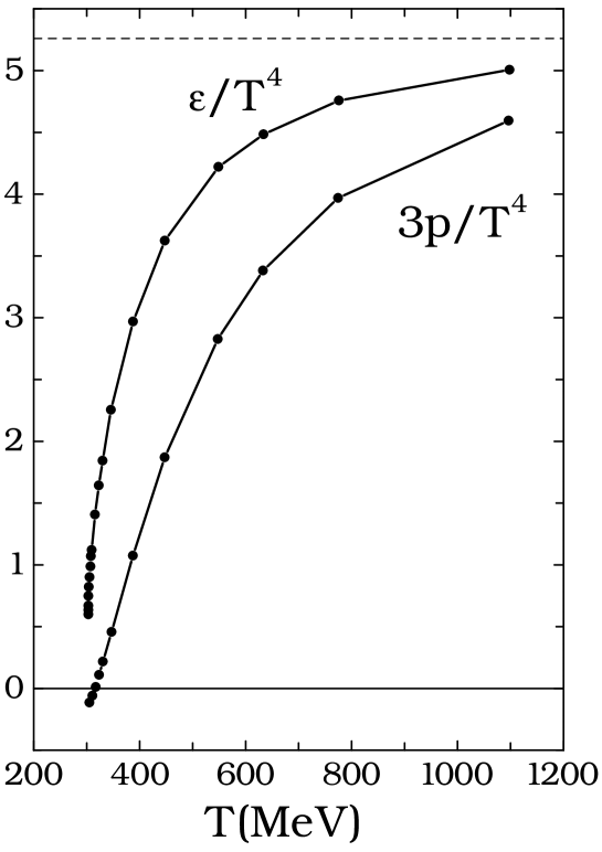
Figure 1: Normalized energy density and pressure of a massless gluon gas with string-like interaction. Dashed line demonstrates the Stephan-Boltzmann regime corresponding to the case of a gas of noninteracting gluons.

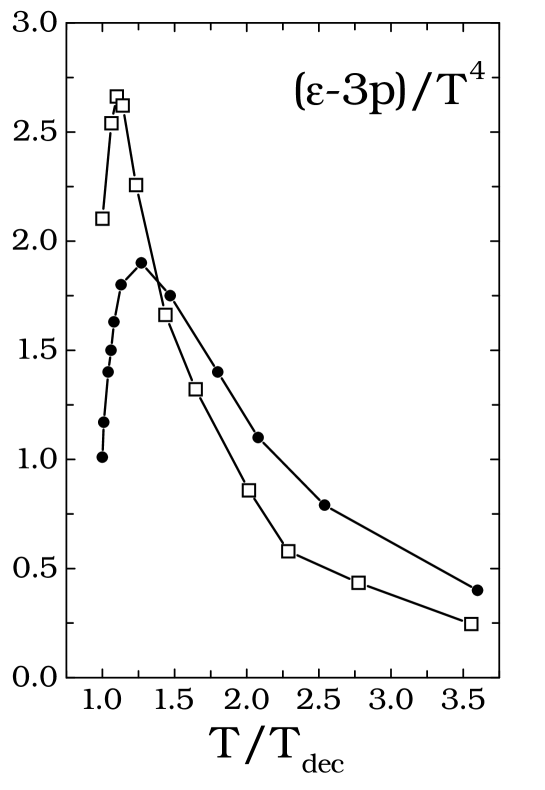
Figure 2: The interaction measure $(\varepsilon-3p)/T^{4}$ of the $SU(3)$ gluon system: circles are our data for the massless gluons interacting via screened strings; squares show the lattice results from Ref.[32]. Our data are plotted for the case $T_{\rm dec}=303\;MeV$.

In Fig. 1 the quantities $\varepsilon/T^{4}$ and $3p/T^{4}$ are plotted as functions of the temperature for the system of gluons with the spectrum Eq. (66) beyond the Boltzmann approximation. As it is seen, Eq. (80) indeed provides a good estimation for the limiting temperature $T_{\rm chem}$, which is now $303$ MeV. The deviation of the pressure and energy curves from the ideal-gas value reflects essential attraction even at $\approx 2T_{c}$. It is now interesting to clarify to what extent our treatment of the in-medium string interactions agrees with the nonperturbative lattice QCD. This can be understood with the help of the special quantity $(\varepsilon-3p)/T^{4}$ that is often called the interaction measure. This quantity is directly related to remnant interactions that survive in the high-temperature QCD phase because for the ideal massless quarks and gluons $\varepsilon=3p$, as mentioned above. In Fig.2 the interaction measure for the $SU(3)$ gluon plasma is shown. As is seen, our treatment of the in-medium strings provides quite reasonable results. The quantity $(\varepsilon-3p)/T^{4}$ turns out to be very sensitive to the QCD interactions. Indeed, it is still equal to zero even in the one-gluon-exchange approximation provided the temperature dependence of the running coupling constant is neglected. The agreement with the lattice calculations could be even better if we chose $\gamma\approx 2/3$ like in Ref. [33]. Thus, the interesting question arises what additional arguments, being able to change the $\gamma$-value from $1/3$ to $2/3$, should be taken into account for our picture of the in-medium string screening. In this respect the spatial correlations of color charges may be of importance (see Sec. 3).

In the transchemistry [11] the reduced effective value $\sigma=0.5\ GeV/fm=0.1\ GeV^{2}$ is used which results in $T_{{\rm chem}}=185\ MeV.$ It seems that the transchemistry model starts at slightly lower temperature where the chemical equilibrium for the quarks would not be possible at all. On the other hand, this simulation begins with a huge oversaturation of the quark number, so a later reheating of the system brings the massive quark matter in an over-critical state. Eventually, expansion and cooling leads to dynamical hadronization at low temperatures ($T<T_{{\rm chem}})$, where the quark component cannot be in chemical equilibrium any more.

Now, returning to the Boltzmann statistics, for the critical number density we have

$$n_{\rm chem}=(\frac{2\lambda}{9e}\ \sigma)^{3/2}\ .$$ (81)

Substituting this quantity into Eq. (70) and taking $\gamma=1/3$,$\;A=(2/3)\sigma$, we get a negative pressure,

$$p_{\rm chem}=-\frac{2\lambda}{81e}\sigma^{2}\ ,$$ (82)

at the critical point. It means that the mechanical equilibrium ceases at a somewhat higher temperature than the chemical one.

Equations similar to Eq. (76) were considered by Boal, Schachter, Woloshin [15] and by Moskalenko and Kharzeev [17], as well. However, investigation of the quark plasma at zero baryon density, presented in the latter paper, did not take into account the important background term $\Phi$. As to the former one, only the boundary for the high-temperature QCD phase, rather than the full thermodynamics, was studied without any reference to the problem of thermodynamical consistency. This is why one of the considered spectrum of unbound partons in this paper is not consistent with Eqs. (21) and (22). In addition, none of these papers uses the relevant classical approximation providing analytical results like Eqs. (79), (81) and (82), which would have significantly simplified understanding. At last, an advantage of our treatment is that it is based on the elaborated model of the in-medium string formation that enables us to derive the mean-field term (51) rather than postulate it invoking the nearest-neighbor approximation inspired by the analogy with the Ising model (see the third paper in Ref. [15]).

4.5 Fermions with string interaction

Another interesting case is massless quarks at zero temperature. The number density integral is given by

$$n=\frac{d}{2\pi^{2}}\int\Theta(\mu-\frac{2}{3}\sigma n^{-1/3}-k)\;k^{2}\,dk\ .$$ (83)

Here $d$ is the color, light flavor and spin degeneracy factor, $\Theta(x)$ denotes the Heaviside step function. Expression (83) can be readily rewritten as

$$n=\zeta^{3}\ \left(\mu-\frac{2}{3}\sigma\ n^{-1/3}\right)^{3}$$

with $\zeta=(d/6\pi^{2})^{1/3}$. In the situation considered we have one conserved charge: the baryon number with the density $n_{b}=n/3$. Then, the chemical equilibrium is specified by the relation $\mu=\mu_{b}/3$, where $\mu_{b}$ is the baryon chemical potential (see Sec. 2). The magnitude of $\mu_{b}$ is determined by the equation

$$n_{b}=\frac{\zeta^{3}}{81}\left(\mu_{b}-\frac{2}{3^{1/3}}\ \sigma\ n_{b}^{-1/3}\right)^{3}.$$ (84)

Using $z=\zeta n_{b}^{-1/3}/3^{3/4}$ we get

$$\frac{1}{z}=\mu-\widetilde{\sigma}_{1}\ z$$ (85)

with $\widetilde{\sigma}_{1}=6\sigma/\zeta.$ Equation (85) has a solution provided

$$\mu_{b}\geq\mu_{{\rm chem}}=2\sqrt{\widetilde{\sigma}_{1}},$$ (86)

i.e. the chemical potential (Fermi energy) is larger than the minimum value of $(\widetilde{\sigma}_{1}z+1/z)$. It means that the Fermi energy of quarks should be larger than $2\sqrt{\widetilde{\sigma}_{1}}/3$. A typical numerical value, $\mu_{{\rm chem}}\approx 2.442$ GeV, can be found using $d=12$ and $\sigma=0.18$ GeV².

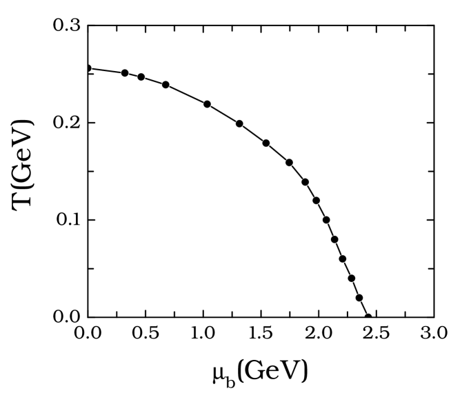
Figure 3: The critical curve on the temperature-chemical potential plane, below which chemical equilibrium ceases for a massless quark gas with string-like interaction.

At finite temperature we obtain a $T$- and $\mu_{b}$-dependent consistency equation, which can be solved only numerically. Fig.3 shows the resulting boundary in the $T$ – $\mu_{b}$ plane.

4.6 Chemical off-equilibrium in the classical approximation

If an isolated system is out of chemical equilibrium and expands as a perfect fluid, the relation

$$dE+p\ dV=T\ dS+\sum_{i}\mu_{i}\ dN_{i}=0\$$ (87)

is fulfilled and the entropy production rate

$$\dot{S}=-\sum_{i}\frac{\mu_{i}}{T}\,\dot{N_{i}}\$$ (88)

is either positive or zero. This means that in the one-component case for quasiparticles with positive $\mu$, the corresponding particle number $N=Vn$ decreases while it increases for negative values of $\mu$.

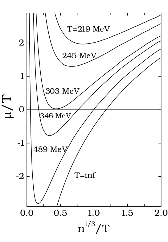
Figure 4: The scaled chemical potential $\mu/T$ as a function of $n^{1/3}/T$ for massless Boltzmann gas with string-like interaction. The chemical equilibrium condition is $\mu=0$.

Fig.4 shows the off-equilibrium chemical potential scaled with the temperature, $\mu/T,$ as a function of the scaled density $n^{1/3}/T$ for a one-component, massless Boltzmann gas made of particles with the $SU(3)$-gluon degrees of freedom and interacting via strings. Chemical equilibrium corresponds to $\mu=0$, which is not reachable below a certain temperature. Then the strings pull the charges together never reaching a screened equilibrium state: the chemical potential remains positive driving the density of this component towards zero.

The situation is more complicated in a many-component mixture due to possible constituent exchange between different species of quasiparticles. In both cases the chemical equilibrium, corresponding to $\mu_{i}=0$, is stable. In some special cases for non-ideal EoS it may happen that the $\mu(n,T)$ curve for a constant $T$ (isoterm) does not cross the $\mu=0$ line at all, i.e. no chemical equilibrium is possible and the system is driven towards a state with either zero or infinite particle numbers. In a many-component system it means that this particular component will dominate or vanish in the mixture.

Another remark concerns with the chemical potential assigned to the conserved charges (e.g. baryon number). This is a physically different situation when the term $-\mu_{b}Q_{b}$ (see Sec. 2) is added to the Hamiltonian, which is not compensated by its expectation value in the background field. As a consequence, the chemical equilibrium point (if any) is placed not at $\mu=0$ but at $\mu=\mu_{B}$. This situation is quite accustom in nuclear physics.

5 Conclusions

A useful representation of the conditions of thermodynamical consistency of quasiparticle description, Eqs. (21) and (22), has been found. The advantage of this representation is that it directly involves the effective quasiparticle spectra, which results in important restrictions to the form of these spectra. In particular, two essential findings can be mentioned. If the interaction with surrounding matter is taken into account by introducing a mean field, the latter should be either temperature independent (Example 1, Sec.2) or, when in-medium effects are included into the Hamiltonian by means of the effective mass (Example 2, Sec. 2), this mass should depend on the temperature or/and the quasiparticle density exclusively through the scalar density of quasiparticles. On the large market of available phenomenological models these general restrictions in majority of cases were used intuitively, but sometimes were erroneously missed.

The structure of the thermodynamical potential, derived from the medium-dependent Hamiltonian in a thermodynamically consistent way, has been further detailized by implementing the string picture for the interaction between generic constituents. With this aim the elaborated mean-field model of the in-medium string interactions has been developed. This model supports the use of the inverse power of the color charge density in the color mean field (see Eq. (51)) that was introduced earlier by various authors assuming validity of the nearest neighbour approximation [15, 16, 17]. Results of our treatment of the in-medium strings are found to be in reasonable agreement with the lattice data on QCD thermodynamics. Further probing of these interactions can be an application of the developed equation of state to (hydro)dynamical calculations allowing direct comparison with observables. Some steps towards this direction have been done recently by analyzing the excitation function for nucleon directed flow [34] and the relation of the ’softest point’ of equation of state with chemical freeze-out [35] in heavy ion collisions.

Along with other results, we would like to comment on the excluded volume modification of the single particle energy. In our treatment the conditions $C_{T}=0,\ C_{1}=0$ have no solution in this case without some additional assumptions. A resolution of this issue has been done in Ref. [8] and in the first paper of Ref. [12].

Acknowledgments
This work has been supported by the Hungarian National Fund for Scientific Research OTKA (project No. T034269). A.A.S. and V.D.T. are grateful to KFKI Research Institute and the heavy-ion group of Prof. Zimanyi for the kind hospitality during their visits to Hungary supported by the Fund for scientific collaborations MTA-Dubna. V.D.T. was also partially supported by DFG (project 436 Rus 113/558/0) and RFBR (grant 00-02-04012-NNIO).

Discussions with B. Müller, D. Blaschke, D. Rischke, J. Zimányi and P. Lévai are gratefully acknowledged.

Figure Captions

Fig.1. Normalized energy density and pressure of a massless gluon gas with string-like interaction. Dashed line demonstrates the Stephan-Boltzmann regime corresponding to the case of a gas of noninteracting gluons.

Fig.2. The interaction measure $(\varepsilon-3p)/T^{4}$ of the $SU(3)$ gluon system: circles are our data for the massless gluons interacting via screened strings; squares show the lattice results from Ref.[32]. Our data are plotted for the case $T_{\rm dec}=303\;MeV$.

Fig.3. The critical curve on the temperature-chemical potential plane, below which chemical equilibrium ceases for a massless quark gas with string-like interaction.

Fig.4. The scaled chemical potential $\mu/T$ as a function of $n^{1/3}/T$ for massless Boltzmann gas with string-like interaction. The chemical equilibrium condition is $\mu=0$.

References

- [1] F. Karsch, E. Laermann, A. Peikert, C. Schmidt, S. Stickman, Nucl. Phys. Proc. Suppl. 94, 411 (2001); F. Karsch, E. Laermann, A. Peikert, Phys. Lett. B 487, 447 (2000); Nucl. Phys. B 605, 579 (2001).
- [2] A. Chodos, R. L. Jaffe, K. Johnson, C. B. Thorn, Phys. Rev. D 10, 2599 (1974); K. Johnson, C. B. Thorn, Phys. Rev. D 13, 1934 (1976); K. Johnson, Phys.Lett. B 78, 259 (1978); J. F. Donoghue, K. Johnson, Phys. Rev. D 21, 1975 (1980); P. Hasenfratz, J. Kuti, Phys. Rept. 40, 75 (1978); B. K. Patra, C. P. Singh, Z. Phys. C 74, 699 (1997); R. Hofmann, T. Gutsche, M. Schumann, R. D. Viollier, Eur. Phys. J. C 16, 677 (2000).
- [3] R. Giles, Phys. Rev. D 13, 1670 (1976).
- [4] G. A. Miller, A. W. Thomas, S. Theberge, Phys. Lett. B 91, 192 (1980); S. Theberge, A. W. Thomas, G. A. Miller, Phys. Rev. D 22, 2838 (1980); ibid 23, 2106 (1981); A. W. Thomas, S. Theberge, G. A. Miller, Phys. Rev. D 24, 216 (1981); S. Lee, K. J. Kong, Phys. Lett. B 202, 21 (1988); G. G. Bunatian, Yad. Fiz. 49, 1071 (1989);ibid 1363 (1989)) (translated as Sov. J. Nucl. Phys. 49, 664 (1989); ibid 847 (1989)); Y. Futami, S. Akiyama, Prog. Theor. Phys. 84, 377 (1990); G. A. Miller, A. W. Thomas, Phys. Rev. C 56, 2329 (1997).
- [5] P. Levai, U. Heinz, Phys. Rev. C 57, 1879 (1998).
- [6] A. Peshier, B. Kämpfer, G. Soff, Phys. Rev. C 61, 045203, 2000; B. Kämpfer, A. Peshier, G. Soff, J. Phys. G 27, 535 (2001).
- [7] J. Rafelski, R. Hagedorn, QCD161:177:1980 (Symposium on Statistical Mechanics of Quarks and Hadrons, Bielefeld, Germany, August 24-31, 1980); ibid, Phys. Lett.B 97, 136 (1980); ibid, QCD161:W7:1978 (Workshop on Hadronic Matter at Extreme Energy Density, Erice, Italy, Oct.13-21, 1978).
- [8] J. Cleymans, M. I. Gorenstein, J. Stalnacke, E. Suhonen, Phys. Scr. 48, 277 (1993); V. K. Tiwari, N. Prasad, C. P. Singh, Phys. Rev. C 58, 439 (1998); V. K. Tiwari, K. K. Singh, N. Prasad, C. P. Singh, Nucl. Phys. A 637, 159 (1998); M. I. Gorenstein, A. P. Kostyuk, Y. D. Krivenko, J. Phys. G 25, L75 (1999); A. Kostyuk, M. I. Gorenstein, S. Stoecker, W. Greiner, Phys. Rev. C 63, 044901 (2001).
- [9] E. G. Nikonov, V. D. Toneev, A. A. Shanenko, Yad. Fiz. 62, 1301 (1999) (translated as Phys. Atom. Nucl. 62, 1226 (1999)); E. Nikonov, A. Shanenko and V. Toneev, Heavy Ion Physics 8, 89 (1998).
- [10] H. W. Barz, B. L. Friman, J. Knoll, H. Schulz, Nucl. Phys. A 484, 661 (1988); ibid Phys. Rev. D 40, 157 (1989); ibid Phys. Lett. B 242, 328 (1990); ibid Nucl. Phys. A 519, 831 (1990).
- [11] T. S. Biró, P. Lévai, J. Zimányi, J. Phys. G 25, 1311 (1999); ibid Phys. Rev. C 59, 1574 (1999).
- [12] A. A. Shanenko, E. P. Yukalova, V. I. Yukalov, Physica A 197, 629 (1993); ibid Yad. Fiz.56, 151 (1993) (translated as Phys. Atom. Nucl. 56, 372 (1993)).
- [13] M. I. Gorenstein, S. N. Yang, Phys. Rev. D 52, 5206 (1995); ibid, J. Phys. G 21, 1053 (1995).
- [14] T. Celik, F. Karsch, H. Satz, Phys. Lett. B 97, 128 (1980); H. Satz, Nucl. Phys. A 642, 130 (1998); S. Fortunato, H. Satz, Phys. Lett. B 475, 311 (2000); S. Fortunato, F. Karsch, P. Petreczky, H. Satz, Nucl. Phys. Proc. Suppl. 94, 204 (2001).
- [15] K. A. Olive, Nucl. Phys. B 190, 483 (1981); ibid. 198, 461 (1982); D. H. Boal, J. Schachter, and R. M. Woloshin, Phys. Rev. D 26, 3245 (1982).
- [16] D. Blaschke, F. Reinholz, G. Röpke, D. Kremp, Phys. Lett. B 151, 439 (1985).
- [17] M. Plumer, S. Raha and R.M. Weiner, Nucl. Phys. A 418, 549(1984); V. V. Balashov, I. V. Moskalenko and D. E. Kharzeev, Yad. Fyz. 47, 1740 (1988)) (translated as Sov. J. of Nucl. Phys. 47, 1103 (1988)); I. V. Moskalenko and D. E. Kharzeev, Yad. Fiz.48, 1122 (1988) (translated as Sov. J. of Nucl. Phys. 48, 713 (1988)).
- [18] S. Kagiyama, A. Minaka and A. Nakamura, Prog. Theor. Phys. 89, 1227 (1993); ibid 95, 793 (1996); ibid, hep-ph/0101036; ibid, hep-ph/0202108.
- [19] D. H. Rischke, M. I. Gorenstein, H. Stöcker and W. Greiner, Z. Phys. C 51, 485 (1991); Q. R. Zhang, Z. Phys. A 351, 89 (1995).
- [20] N. Prasad, K. K. Singh, and C. P. Singh, Phys. Rev. C 62, 037903 (2000).
- [21] N. N. Bogoliubov, N. N. Bogoliubov, Jr., Introduction to Quantum Statistical Mechanics (World Scientific, Singapore,1982), see Secs. 3.4.1 and 3.4.2.
- [22] U. Heinz, W. Greiner, W. Scheild, J. Phys. G 5, 1383 (1979); U. Heinz, P. R. Subramanian, H. Stöcker and W. Greiner, J. Phys. G. 12, 1237 (1986).
- [23] J. I. Kapusta, K. A. Olive, Nucl. Phys. A 408, 478 (1983).
- [24] J. Zimányi, B. Lukács, P. Lévai, J. P. Bondorf, N. L. Balázs, Nucl. Phys. A 484, 647 (1988).
- [25] D. V. Anchishkin, Sov. Phys. JETP 75, 195 (1992); D. Anchishkin and E. Suhonen, Nucl. Phys. A 586, 734 (1995); V. K. Tiwary, N. Prasad and C. P. Singh, Phys. Rev. C 58, 439 (1998).
- [26] J. D. Walecka, Ann. Phys.(N.Y.) 83, 491 (1974); ibid, Phys. Lett. B 59, 109 (1975).
- [27] V. Goloviznin, H. Satz, Z. Phys. C 57, 671 (1993).
- [28] D. H. Rischke, Nucl. Phys. A 583, 663 (1995).
- [29] Bi Pin-zhen, Shi Yao-ming, Z. Phys. C. 75, 735 (1997).
- [30] A. A. Shanenko, Phys. Rev. E 54, 4420 (1996).
- [31] E. Suhonen, J. Cleymans, J. Stalnacke, Nucl. Phys. Proc. Suppl. B 24, 260 (1991); J. Cleymans, M. Marais, E. Suhonen, Phys. Rev. C 56, 2747 (1997); A. Keranen, J. Cleymans, E. Suhonen, J. Phys. G 25, 275, (1999).
- [32] G. Boyd et al., Nucl. Phys. B 469, 419 (1996).
- [33] V. D. Toneev, E. G. Nikonov, and A. A. Shanenko, in Nuclear Matter in Different Phases and Transitions, eds. J.-P. Blaizot, X. Campi, and M. Ploszajczak (Kluwer A. P., 1999) p.309; Preprint GSI-98-30, Darmstadt, 1998.
- [34] Yu. Ivanov, N. Nikonov, W. Norenberg, A. Shanenko and V. Toneev, Heavy Ion Phys. 15, 117 (2002).
- [35] V. Toneev, J. Cleymans, E. Nikonov, K. Redlich, A. Shanenko, J. Phys. G 27, 827 (2001).