Polarization observables in the reaction $pn\to d\phi$

Abstract

The reaction $pn\to d\phi$ is studied within a covariant boson exchange model. The behavior of polarization observables being accessible in forthcoming experiments near threshold is predicted.
PACS. 13.75.-n Hadron-induced low- and intermediate-energy reactions and scattering (energy $\leq$ 10 GeV) – 14.20.-c Baryons (including antiparticles) – 21.45.+v Few-body systems

I Introduction

Data on elementary reactions with neutrons are scare since either they must be extracted, with some efforts and even mostly with some model dependent assumptions, from reactions on nuclei, or a tagged neutron beam (cf. [1]) is used. The spectator technique [2, 3] represents one example how one can use a deuteron target to isolate quasi-free reactions at the neutron. It is based on the idea to measure the spectator proton ($p_{\rm sp}$) at fixed (or slightly varying) beam energy in the meson ($M$) production reactions $pd\to dMp_{\rm sp}$ thus exploiting the internal momentum spread of the neutron inside the deuteron ($d$). In such a way one gets access to quasi-free reactions $pn\to dM$ if, in experiments with the deuteron target at rest, the spectator proton has momenta in the order of 50 $\cdots$ 150 MeV/c.

An experimental investigation of the threshold-near (pseudo)scalar and vector meson production at the neutron becomes therefore feasible. Indeed, at COSY the ANKE spectrometer set-up can be used, in particular, for studying the $a_{0}$, $\omega$ and $\phi$ production with the internal beam at a ”neutron target” [3]. This offers the possibility to enlarge the data base on hadronic reactions and to address special issues. For instance, there is already a large body of data which can be used for a systematic study of the OZI rule violation via $\omega$ and $\phi$ production in $\pi N$ and $pp$ reactions (cf. [4] for a reanalysis) and in $\bar{p}p$ annihilation (cf. [5, 6] for theoretical analyzes) as well. OZI rule violations are of interest with respect to possible hints to a significant $s\bar{s}$ admixture in the proton, as supported by the pion-nucleon $\Sigma$ term [7, 8] and interpretations of the lepton deep-inelastic scattering data [9]. Besides the impact on hadron phenomenology the origin of the OZI rule has also a link to QCD [10, 11].

In the reactions $pp\to ppM$ or $pn\to pnM$ the final state interaction among the outgoing nucleons plays a role. Therefore, the meson production process is a convolution of the ”pure production process” and the final state interaction. In the case of the reaction $pn\to dM$ one has one well defined final state of the nucleons and may better constrain the elementary production amplitude.

Finally, we mention that in the reactions $pp\to ppM$, $pn\to pnM$ and $pn\to dM$ the conservation laws and symmetry principles determine a different dynamics near threshold, which needs to be investigated to allow a firm understanding of the reactions and the systematics of the OZI rule violation.

Given this motivation, in [12, 13] the reaction $pn\to dV$ with $V=\omega,\phi$ has been studied in some detail. ($pn\to dS$ with $S=a_{0}^{+},\eta,\eta^{\prime}$ is considered in [14].) In [12] the cross sections and angular distributions are elaborated as a function of the excess energy within a two-step model. The same observables are evaluated in [13] within the framework of a boson exchange model with emphasis on the ratio of cross sections $\sigma_{pn\to d\phi}/\sigma_{pn\to d\omega}$ being of direct relevance for the OZI rule violation.

Since at COSY the proton beam is polarized and also polarized targets are envisaged, we extend the previous studies [12, 13] to make a prediction of polarization observables in the reaction $pn\to d\phi$. The set-up of the ANKE experiment at COSY can directly identify the $\phi$ via its $K^{+}K^{-}$ decay channel. We present the asymmetry, tensor analyzing power, and proton-phi spin-spin correlations. In doing so we use our previous one-boson exchange model [15] with parameters adjusted to available threshold-near data on $\phi$ production in $pp$ and $\pi p$ reactions and combine this with our previous studies [15, 16, 17] employing a solution of the deuteron wave function within the Bethe-Salpeter (BS) formalism. In this way we derive a completely covariant approach with correct treatment of the off-shell effects in the $\pi N\to\phi N$ subprocess amplitudes.

Extensions to $pn\to d\omega$ and even to $pd\to dVp_{sp}$ are much more involved and, therefore, relegated to separate work.

Our paper is organized as follows. In section 2 we present the theoretical framework and elaborate the basic equations. The numerical results and their discussion are presented in section 3. The summary can be found in section 4.

II The model

The invariant differential cross section of the reaction $pn\to d\phi$ reads

$$\frac{d\sigma}{dt}=\frac{1}{16\pi\,s(s-4m^{2})}\,\frac{1}{4}\sum\limits_{s_{1},s_{2}}\sum\limits_{{\cal M}_{\phi},{\cal M}_{d}}\,|T_{s_{1}s_{2}}^{{\cal M}_{\phi}{\cal M}_{d}}(s,t)|^{2},$$ (1)

where $s$ is the square of the total energy of the colliding particles p and n in the center of mass, $t$ is the square of the transfered 4-momentum, $m$ is the nucleonic mass, $s_{1},s_{2},{\cal M}_{\phi}$ and ${\cal M}_{d}$ denote the spin projections on a given quantization axis, and $T$ stands for the invariant amplitude. The general form of $T$ may be written in the form (cf. Fig. 1) $T_{s_{1}s_{2}}^{{\cal M}_{\phi}{\cal M}_{d}}(s,t)=\langle\,d,{\cal M}_{d}\,|\hat{G}_{\mu}\,\xi^{*\mu}_{{\cal M}_{\phi}}|1,2\,\rangle,$ where $\xi^{\mu}_{{\cal M}_{\phi}}$ is the polarization 4-vector of the $\phi$ meson. The scattering operator $\,\hat{G}\,\,$ represents a 4-vector in Minkowski space, a vector in the vector space of mesons and a $16\otimes 16$ component object in the spinor space of nucleons. The deuteron is described as a $16$ component BS amplitude $\Phi(1,2)$ which is defined as a matrix element of a time ordered product of two nucleon fields $\psi(x)$ by $\Phi^{\alpha\beta}(1,2)=\langle\,d|{\cal T}\left(\psi^{\alpha}(1)\psi^{\beta}(2)\right)|0\,\rangle$ and satisfies the BS equation. By defining another scattering operator via $\hat{O}=\hat{G}_{\mu}\,\xi^{\mu*}_{{\cal M}_{\phi}}$ the invariant amplitude reads

$$T_{s_{1}s_{2}}^{{\cal M}_{\phi}{\cal M}_{D}}(s,t)=-i\int\,\frac{d^{4}p}{(2\pi)^{4}}\,\bar{\Phi}_{{\cal M}_{d}}^{\alpha b}(1^{\prime},2^{\prime})\,\hat{O}^{bc}_{\alpha\beta}(12;1^{\prime}2^{\prime},{\cal M}_{\phi})\,u^{c}_{s_{1}}(1)\,u^{\beta}_{s_{2}}(2),$$ (2)

where $\bar{\Phi}_{{\cal M}_{d}}^{\alpha b}(1^{\prime},2^{\prime})$ is the conjugate BS amplitude in the momentum space, $p$ is the relative 4-momentum of the nucleons in the deuteron, and $u(1)$ and $u(2)$ denote the Dirac spinors for the incident nucleons. Summation over spin indices $\alpha,\beta,b,c=1\cdots 4$ occurring pairwise is supposed. The operator $\hat{O}^{bc}_{\alpha\beta}(12;1^{\prime}2^{\prime},{\cal M}_{\phi})$ is a scattering operator describing the $\phi$ meson production in the final state. This operator acts in the spinor space of protons and neutrons separately; the upper (Latin) and lower (Greek) spinor indices refer to protons and neutrons, respectively. The first indices, $b$ and $\alpha$, form an outer product of two columns, whereas the second ones, $c$ and $\beta$, form an outer product of two rows. To specify explicitly the spinor structure we decompose the operator $\hat{O}$ in each of its indices over the corresponding complete set of Dirac spinors, i.e,

$$\hat{O}^{bc}_{\alpha\beta}(12;1^{\prime}2^{\prime},{\cal M}_{\phi})=\frac{1}{(2m)^{4}}\sum\limits_{r,r^{\prime},\rho,\rho^{\prime}=1}^{4}\,A_{rr^{\prime},\rho\rho^{\prime}}^{{\cal M}_{\phi}}(12;1^{\prime}2^{\prime})u^{b}_{r^{\prime}}(1^{\prime})\bar{u}^{c}_{r}(1)\bar{u}^{\beta}_{\rho}(2)u^{\alpha}_{\rho^{\prime}}(2^{\prime}),$$ (3)

where the coefficients $A_{rr^{\prime},\rho\rho^{\prime}}^{{\cal M}_{\phi}}(12;1^{\prime}2^{\prime})$ may be found by using the completeness and orthogonality of the Dirac spinors, $\bar{u}_{r}({\bf p})u_{r^{\prime}}({\bf p})=2\varepsilon_{r}m\delta_{rr^{\prime}}$, yielding

$$A_{rr^{\prime},\rho\rho^{\prime}}^{{\cal M}_{\phi}}(12;1^{\prime}2^{\prime})=\varepsilon_{r}\varepsilon_{r^{\prime}}\varepsilon_{\rho}\varepsilon_{\rho^{\prime}}\,\bar{u}^{b}_{r^{\prime}}(1^{\prime})\,\bar{u}^{\alpha}_{\rho^{\prime}}(2^{\prime})\,\hat{O}^{bc}_{\alpha\beta}(12;1^{\prime}2^{\prime},{\cal M}_{\phi})\,u^{c}_{r}(1)\,u^{\beta}_{\rho}(2),$$ (4)

where $\varepsilon_{r}=+1$ for $r=1,2$ and $\varepsilon_{r}=-1$ for $r=3,4$. Substituting (3) into (2) one obtains

$$T_{s_{1}s_{2}}^{{\cal M}_{\phi}{\cal M}_{d}}(s,t)=\frac{-i}{(2m)^{2}}\int\,\frac{d^{4}p}{(2\pi)^{4}}\bar{\Phi}_{{\cal M}_{D}}^{\alpha b}(1^{\prime},2^{\prime})\,\sum\limits_{r,r^{\prime}=1}^{2}A_{s_{1}s_{2},rr^{\prime}}^{{\cal M}_{\phi}}(12;1^{\prime}2^{\prime})\,u^{\alpha}_{r^{\prime}}(2^{\prime})u^{b}_{r}(1^{\prime})$$ (5)

$$=\frac{i}{(2m)^{2}}\sum\limits_{r,r^{\prime}=1}^{2}\int\,\frac{d^{4}p}{(2\pi)^{4}}\left(u^{\alpha}_{r^{\prime}}(2^{\prime})\right)^{T}\gamma_{c}^{\alpha\alpha^{\prime}}\left(\gamma_{c}^{\alpha^{\prime}\alpha^{\prime\prime}}\bar{\Phi}_{{\cal M}_{d}}^{\alpha^{\prime\prime}b}(1^{\prime},2^{\prime})\right)\,A_{s_{1}s_{2},rr^{\prime}}^{{\cal M}_{\phi}}(12;1^{\prime}2^{\prime})u^{b}_{r}(1^{\prime})$$ (6)

$$=\frac{i}{(2m)^{2}}\sum\limits_{rr^{\prime}=1}^{2}\int\,\frac{d^{4}p}{(2\pi)^{4}}A_{s_{1}s_{2},rr^{\prime}}^{{\cal M}_{\phi}}(12;1^{\prime}2^{\prime})\bar{v}_{r^{\prime}}(2^{\prime})\bar{\Psi}_{{\cal M}_{d}}(1^{\prime},2^{\prime})u_{r}(1^{\prime}),$$ (7)

where $\gamma_{c}$ is the charge conjugation matrix, $\bar{v}_{r}(2^{\prime})\equiv(u_{r}(2^{\prime}))^{T}\gamma_{c}$, and the new BS amplitude $\bar{\Psi}_{{\cal M}_{d}}(1^{\prime},2^{\prime})\equiv\gamma_{c}\bar{\Phi}_{{\cal M}_{d}}(1^{\prime},2^{\prime})$ now is a $4\otimes 4$ matrix and represents the solution of the BS equation written also in matrix form.

For further evaluations of the amplitude (7) one needs to specify an explicit form of the operator $\hat{O}$. Following [15], and taking into account only the meson-exchange contribution from one-boson exchange diagrams with internal meson conversion, the operator $\hat{O}$ may be represented by four truncated diagrams as depicted in Fig. 2. (The contributions of the nucleonic currents are found to be negligibly small [13, 15] and, therefore, can be omitted for many purposes.) Consequently, having computed the operator $\hat{O}$ by using the effective interaction Lagrangians for the $\pi NN$, $\rho NN$, $\phi\rho\pi$ vertices and monopole form factors for dressing the vertices as in [15], it is straightforward to obtain the coefficients $A_{rr^{\prime},\rho\rho^{\prime}}^{{\cal M}_{\phi}}(12;1^{\prime}2^{\prime})$ in (4). If all particles were on mass shell, $A_{rr^{\prime},\rho\rho^{\prime}}^{{\cal M}_{\phi}}(12;1^{\prime}2^{\prime})$ exactly coincides with the amplitude of the elementary process $1+2\to 1^{\prime}+2^{\prime}+\phi$. However, in general case this amplitude corresponds to a virtual process of vector meson production with two off-shell nucleons in the final state.

Since our numerical solution [18] of the BS equation has been obtained in the deuteron’s center of mass, all further calculations will be performed in this system. First, as depicted in Fig. 1, we introduce the relevant kinematical variables as follows: $p_{1,2}$ are the 4-momenta of incoming nucleons, $p_{1,2}^{\prime}$ stand for the 4-momenta of the internal (off-shell) nucleons in the deuteron with $p=(p_{1}^{\prime}-p_{2}^{\prime})/2$; $\xi_{{\cal M}_{d}}$ denotes the polarization 4-vector of the deuteron. In this notation the BS amplitudes in the deuteron’s rest system are of the form [17]

$$\!\!\!\!\!\Psi_{{\cal M}_{d}}^{S^{++}}(p_{1}^{\prime},p_{2}^{\prime})={\cal N}(\hat{k}_{1}+m)\frac{1+\gamma_{0}}{2}\hat{\xi}_{{\cal M}_{d}}(\hat{k}_{2}-m)\phi_{S}(p_{0},|{\bf p}|),$$ (8)

$$\!\!\!\!\!\Psi_{{\cal M}_{d}}^{D^{++}}(p_{1}^{\prime},p_{2}^{\prime})=-\frac{{\cal N}}{\sqrt{2}}(\hat{k}_{1}+m)\frac{1+\gamma_{0}}{2}\left(\hat{\xi}_{{\cal M}_{d}}+\frac{3}{2|{\bf p}|^{2}}(\hat{k}_{1}-\hat{k}_{2})(p\xi_{M})\right)(\hat{k}_{2}-m)\phi_{D}(p_{0},|{\bf p}|),$$ (9)

where $\,\hat{}\,$ means contraction with Dirac matrices, and $k_{1,2}$ are on-shell 4-vectors related to the off-shell vectors $p_{1,2}^{\prime}$ as follows

$$k_{1}=(E_{p},{\mbox{\boldmath$p$}}),\quad k_{2}=(E_{p},-{\mbox{\boldmath$p$}}),\quad p_{1}^{\prime}=(p_{10}^{\prime},{\mbox{\boldmath$p$}}),\quad p_{2}^{\prime}=(p_{20}^{\prime},-{\mbox{\boldmath$p$}}),\quad E_{p}=\sqrt{{\mbox{\boldmath$p$}}^{2}+m^{2}},$$ (10)

and $\phi_{S,D}(p_{0},|{\bf p}|)$ are the partial scalar amplitudes, related to the corresponding partial vertices as

$$\phi_{S,D}(p_{0},|{\bf p}|)=\displaystyle\frac{G_{S,D}(p_{0},|{\bf p}|)}{\left(\displaystyle\frac{1}{2}M_{d}-E_{p}\right)^{2}-p_{0}^{2}}.$$ (11)

$M_{d}$ is the deuteron mass, and the normalization factor is ${\cal N}=\left\{\sqrt{8\pi}2E(E+m)\right\}^{-1}$. To be explicit let us recall the components of the polarization 4-vector of a vector particle with 4-momentum $p=(E,{\bf p})$, polarization index ${\cal M}=\pm 1,\,0$ and mass $M$ as

$$\xi_{\cal M}=\left(\frac{\mbox{\boldmath{$p$}}\mbox{\boldmath{$\xi$}}_{\cal M}}{M},\mbox{\boldmath{$\xi$}}_{\cal M}+\mbox{\boldmath{$p$}}\frac{\mbox{\boldmath{$p$}}\mbox{\boldmath{$\xi$}}_{\cal M}}{M(E+M)}\right),$$ (12)

where ${\mbox{\boldmath$\xi$}}_{\cal M}$ is the polarization 3-vector for the particle at rest with ${\mbox{\boldmath$\xi$}}_{+1}=\frac{1}{\sqrt{2}}(1,i,0)$, ${\mbox{\boldmath$\xi$}}_{-1}=\frac{1}{\sqrt{2}}(1,-i,0)$, ${\mbox{\boldmath$\xi$}}_{0}=(0,0,1)$ and the above Dirac spinors, normalized as $\bar{u}(p)u(p)=2m$ and $\bar{v}(p)v(p)=-2m$, read

$$u({\mbox{\boldmath$p$}},s)=\sqrt{m+\epsilon}\left(\begin{array}[]{c}\chi_{s}\\ \frac{{\mbox{\boldmath$\sigma$}}{\mbox{\boldmath$p$}}}{m+\epsilon}\chi_{s}\end{array}\right),\quad\quad v({\mbox{\boldmath$p$}}\,,s)=\sqrt{m+\epsilon}\left(\begin{array}[]{c}\frac{{\mbox{\boldmath$\sigma$}}{\mbox{\boldmath$p$}}}{m+\epsilon}\widetilde{\chi}_{s}\\ \widetilde{\chi}_{s}\end{array}\right),$$ (17)

where $\widetilde{\chi}_{s}\equiv-i\sigma_{y}\chi_{s}$, and $\chi_{s}$ denotes the usual two-dimensional Pauli spinor. In general, the BS amplitude consists on eight partial components. In (8) we take into account only the most important ones, namely the $S$ and $D$ partial amplitudes. The other six amplitudes may become important at high transferred momenta [16, 17], hence for the present near-threshold process they may be safely disregarded. Substituting (8-17) into (7) one obtains after some algebra

$$T_{s_{1}s_{2}}^{{\cal M}_{\phi}{\cal M}_{d}}(s,t)=\frac{-i}{\sqrt{8\pi}}\sqrt{|{\cal M}_{D}|+1}$$ (18)

$$\times\sum\limits_{r,r^{\prime}}\int\,\frac{d^{4}p}{2E_{p}(2\pi)^{4}}\frac{G_{S}-G_{D}\frac{1}{\sqrt{2}}}{\left(\frac{1}{2}M_{d}-E_{p}\right)^{2}-p_{0}^{2}}A_{s_{1}s_{2},rr^{\prime}}^{{\cal M}_{\phi}}({\mbox{\boldmath$p$}}_{1}{\mbox{\boldmath$p$}}_{2},{\mbox{\boldmath$p$}}_{1}^{\prime}{\mbox{\boldmath$p$}}_{2}^{\prime})\,\delta_{r+r^{\prime},{\cal M}_{d}}$$ (19)

$$+\frac{3i}{\sqrt{16\pi}}\sum\limits_{r,r^{\prime}}\int\,\frac{d^{4}p}{2E_{p}(2\pi)^{4}}\frac{G_{D}}{\left(\frac{1}{2}M_{d}-E_{p}\right)^{2}-p_{0}^{2}}A_{s_{1}s_{2},rr^{\prime}}^{{\cal M}_{\phi}}({\mbox{\boldmath$p$}}_{1}{\mbox{\boldmath$p$}}_{2},{\mbox{\boldmath$p$}}_{1}^{\prime}{\mbox{\boldmath$p$}}_{2}^{\prime})\widetilde{\chi}^{+}_{r^{\prime}}\,(\mbox{{\boldmath$\sigma$}}{\mbox{\boldmath$n$}})\chi_{r}\,({\mbox{\boldmath$n$}}{\mbox{\boldmath$\xi$}}^{*}_{{\cal M}_{D}}).$$ (20)

where here and below the sums over $r,r^{\prime}$ run from 1 to 2. By closing the integration contour in the upper hemisphere and picking up the residuum at $p_{0}=M_{d}/2-E_{p}$ and introducing the notion of the deuteron $S$ and $D$ wave functions as

$$u_{S}(p)=\frac{G_{S}(p_{0},|{\mbox{\boldmath$p$}}|)}{4\pi\sqrt{2M_{d}}(2E_{p}-M_{d})},\quad u_{D}(p)=\frac{G_{D}(p_{0},|{\mbox{\boldmath$p$}}|)}{4\pi\sqrt{2M_{d}}(2E_{p}-M_{d})}$$ (21)

with $2\int d\,|{\mbox{\boldmath$p$}}|\,|{\mbox{\boldmath$p$}}|^{2}(u_{S}^{2}+u_{D}^{2})\approx\pi$, the final expression for the amplitude may be written as

$$T_{s_{1}s_{2}}^{{\cal M}_{\phi}{\cal M}_{d}}(s,t)=\sqrt{\frac{M_{d}}{4\pi}}\sum\limits_{rr^{\prime}}\int\,\frac{d^{3}{\mbox{\boldmath$p$}}}{E_{p}(2\pi)^{2}}A_{s_{1}s_{2},rr^{\prime}}^{{\cal M}_{\phi}}({\mbox{\boldmath$p$}}_{1},{\mbox{\boldmath$p$}}_{2};{\mbox{\boldmath$p$}},-{\mbox{\boldmath$p$}})$$ (22)

$$\times\left\{\sqrt{|{\cal M}_{d}|+1}\left[u_{S}(p)-\frac{u_{D}(p)}{\sqrt{2}}\right]\delta_{r+r^{\prime},{\cal M}_{d}}-3\frac{u_{D}(p)}{\sqrt{2}}\left({\mbox{\boldmath$\xi$}}^{*}_{{\cal M}_{d}}{\mbox{\boldmath$n$}}\right)\,\widetilde{\chi}_{r^{\prime}}^{+}(\mbox{{\boldmath$\sigma$}}{\mbox{\boldmath$n$}})\chi_{r}\right\},$$ (23)

where $n$ is a unit vector parallel to $p$.

III Discussion of results

In our evaluation of the above equations we use, for describing the deuteron wave function [18], the numerical solution of the BS equation in ladder approximation obtained with a realistic one-boson exchange interaction which includes $\pi,\sigma,\omega,\delta,\rho$ and $\eta$ exchanges. The effective parameters used in the ladder approximation have been fixed in such a way to obtain a good description of the $NN$ elastic scattering data and the static properties of the deuteron [17]. Independent of this set of parameters related to deuteron properties, the effective coupling constants and the attributed cut-off factors are taken from the recent analysis [15]. In all subsequent numerical calculations, the set B from [15] is used. For this parameter set the meson exchange term is by far dominating. In Fig. 3 the total cross section near the threshold is depicted. The shape of our cross section is rather similar to the one computed in [13]. However, there is a difference in the absolute values by roughly a factor of $2/3$. This difference is in the same order of magnitude as the difference of the previously often used cross section $\sigma=0.26$ $\mu$b deduced from [19] and the published value $\sigma=0.19$ $\mu$b [20] for the reaction $pp\to pp\phi$ at an excess energy of 83 MeV.

Refs. [13, 15] show that several sets of parameters equally well describe the $pp\to pp\phi$ data. These sets differ not only by absolute values of parameters but also by the relative contributions of meson current and the nucleon current terms. Since in case of the $pn\to d\phi$ processes the isospin transition corresponds to $\Delta I=0$ the meson-exchange diagrams are enhanced by a factor of three in comparison with the nucleon current terms. This means that (i) the contributions of the nucleon current are suppressed by about one order of magnitude in comparison with the meson current, and (ii) the behavior of the cross section and angular distribution in the process $pn\to d\phi$ is expected to follow essentially the behavior of the dominating meson-exchange current contribution in the elementary processes $pn\to pn\phi$. The occurrence of the deuteron wave function will only modify this behavior. This is clearly seen in Fig. 4, where the behavior of the angular distribution is very similar to the distribution found in [15] for the reaction $pn\to pn\phi$. At the threshold the distribution is fairly flat, while with increasing excess energy some forward-backward peaking becomes visible. This feature depends upon the parameter set used. For instance, if we were using the set C of [15], then a slight suppression of the cross section would be expected in the forward-backward directions as predicted for the elementary cross section [15]. This sensitivity of the predicted angular distribution has been pointed out in [13, 21] as a tool to constrain further the parameters, if precise data become available.

Let us now discuss the polarization observables. Near the threshold, in the final state one has: $I_{f}=0$, $L_{f}=0,2$, $J_{f}^{\pi}=J_{\phi}^{\pi}+J_{D}^{\pi}=0^{-},1^{-},2^{-}$, where $I$, $L$ and $J^{\pi}$ are the total isospin, total radial angular momentum, angular momentum and parity, respectively. Thus from symmetry constraints, in the initial state the allowed configurations are $I_{i}=0$, $L_{i}=1,3,5\cdots$ and total spin $S_{i}=0$. The conservation law implies $L_{i}=1$, so that $J_{i}^{\pi}=1^{-}$. From these transitions in $|T_{s_{1}s_{2}}^{{\cal M}_{\phi}{\cal M}_{d}}(s,t)|^{2}$ one may form different combinations of spin observables, which near the threshold behave quite differently. If one considers, for example, the cross section averaged over all final projections ${\cal M}$ at different initial spin projections, then the beam-target asymmetry, defined here as

$${\cal A}=\frac{\sigma(s_{p}+s_{n}=1)+\sigma(s_{p}+s_{n}=-1)-\sigma(s_{p}+s_{n}=0)}{\sigma(s_{p}+s_{n}=1)+\sigma(s_{p}+s_{n}=-1)+\sigma(s_{p}+s_{n}=0)},$$ (24)

is predicted to be $-1$ near threshold and to increase with increasing energy. This is in contrast with the asymmetry defined for the elementary process $pp\to pp\phi$ which is $+1$, as predicted in [15], and decreases with increasing energy. The energy dependence of the asymmetry (24) is depicted in Fig. 5.

Another interesting polarization observable is the tensor analyzing power, which may be defined either for the final deuteron or for the final meson. For instance, the deuteron tensor analyzing power is defined by the cross section averaged over all spins but the deuteron,

$$T_{20}=\frac{1}{\sqrt{2}}\frac{\sigma({\cal M}_{d}=1)+\sigma({\cal M}_{d}=-1)-2\sigma({\cal M}_{d}=0)}{\sigma({\cal M}_{d}=1)+\sigma({\cal M}_{d}=-1)+\sigma({\cal M}_{d}=0)}.$$ (25)

It is seen from (25) that in line with the above discussed selection rules, $\sigma({\cal M}_{d}=0)\ll\sigma({\cal M}_{d}=\pm 1)$ and the deuteron tensor analyzing power is predicted to be almost constant, $T_{20}\approx 1/\sqrt{2}$, in a large region of the energy excess. This prediction is illustrated in Fig. 6.

In Fig. 7 another polarization observable is depicted defined by

$$W_{zz}=\left.\frac{\sigma({\cal M}_{\phi}=+1)-\sigma({\cal M}_{\phi}=-1)}{\sigma({\cal M}_{\phi}=+1)+\sigma({\cal M}_{\phi}=-1)}\right|_{s_{p}=+1/2}$$ (26)

which characterizes the proton-meson spin-spin correlation. This quantity is predicted to vanish near the threshold for the meson exchange diagrams. A substantial deviation of $W_{zz}$ from zero would point to the presence of non-negligible nucleon current contributions in the $\phi$ production process. In Fig. 7 it is seen that there is some weak dependence of $W_{zz}$ upon the energy excess. Nevertheless $W_{zz}$ remains very small indicating that the polarizations of the incident proton and outgoing meson are almost uncorrelated. A different situation will occur in the reaction $pd\to d\phi p_{sp}$. In this case, if one measures also the polarization of the spectator proton, the quantity $W_{zz}$ is expected to strongly depend on whether the polarizations of protons are the same or have opposite directions.

Since we have $T_{s_{1}s_{2}}^{{\cal M}_{\phi}{\cal M}_{d}}(s,t)$ at disposal, via (1) any other polarization observable is accessible within the our formalism and corresponding numerical code.

IV Summary

In summary we present here a evaluation of polarization observables for the process $pn\to d\phi$ which are accessible in forthcoming experiments. Off-shell effects in the sub-process $\pi N\to\phi N$ can correctly be dealt with if one restricts the treatment on the by far dominating meson-exchange current. It is the beam-target asymmetry which differs drastically from the one in the reaction $pp\to pp\phi$. The tensor analyzing power is fairly insensitive to variations of the excess energy, and the proton-phi spin-spin correlation is very small.

The treatment can be extended to incorporate the $\omega$ meson production; work along this line is in progress.

Acknowledgments

We are grateful to A.I. Titov for many valuable discussions. The work is supported in parts by BMBF grant 06DR921 and the Landau-Heisenberg program.

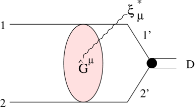
FIG. 1.: The diagram for the process $p(1)+n(2)=d+\phi$. $G$ is the scattering operator, and $\xi^{*}$ denotes the polarization vector of the outgoing vector meson.

FIG. 2.: Graphical representation of the operator $\hat{O}$ defined in (3) in the one-boson exchange approximation. Nucleons in the initial and final states are represented by thin lines which are truncated by vertical dotted lines as to obtain an operator. The exchanged $\pi$ and $\rho$ mesons are depicted by vertical dashed and thick lines, respectively. The four different contributions correspond to different combinations of $\pi^{0},\pi^{\pm}$ and $\rho^{0},\rho^{\pm}$ exchanges.

FIG. 3.: Total cross section for the reaction $pn\to d\phi$ as a function of the excess energy $\Delta s^{1/2}=\sqrt{s}-M_{d}-M_{\phi}$.

FIG. 4.: Angular distribution in the center of mass system for various values of the excess energy.

FIG. 5.: The beam-target asymmetry ${\cal A}$ as a function of the the excess energy.

FIG. 6.: Deuteron tensor analyzing power $T_{20}$ as a function of the excess energy.

FIG. 7.: Proton-phi spin-spin correlation $W_{zz}$ as a function of the excess energy.

REFERENCES

- [1] T. Peterson et al., Nucl. Phys. A 663, 1057c (2000)
-
[2]
H. Calén et al., Phys. Rev. Lett. 79, 2642 (1997),
80 (1998) 2069, Phys. Rev. C 58, 2667 (1998);
R. Bilger et al., Nucl. Phys. A 663, 1053c (2000) - [3] M. Büscher et al., ”Study of and meson production in the reaction at ANKE”, experiment proposal #75/ANKE, http://ikpd15.ikp.kfa-juelich.de:8085/doc/Proposals.html
- [4] A. Sibirtsev, W. Cassing, Eur. Phys. J. A 7, 407 (2000)
- [5] J. Ellis, M. Karliner, D.E. Kharzeev, M.G. Sapozhnikov, Nucl. Phys. A 673, 256 (2000)
- [6] S. von Rotz, M.P. Locher, V.E. Markushin, Eur. Phys. J. A 7, 261 (2000)
- [7] J.F. Donoghue, C.R. Nappi, Phys. Lett. B 168, 105 (1986)
- [8] J. Gasser, H. Leutwyler, M.E. Sainio, Phys. Lett. B 253, 252 (1991)
- [9] J. Ashman et al. Phys. Lett. B 206, 364 (1988)
- [10] N. Isgur, H.B. Thacker, hep-lat/0005006
- [11] T. Schäfer, E.V. Shuryak, hep-lat/0005025
-
[12]
L.A. Kondratyuk, Ye. Golubeva, M. Büscher,
nucl-th/9808050,
V.Yu. Grishina, L.A. Kondratyuk, M. Büscher, nucl-th/9906064. - [13] K. Nakayama, J. Haidenbauer, J. Speth, Phys. Rev. C 63, 015201 (2000)
- [14] V.Yu. Grishina et al., Phys. Lett. B 475, 9 (2000), Eur. Phys. J. A 9, 277 (2000)
- [15] A.I. Titov, B. Kämpfer, B.L. Reznik, Eur. Phys. J. A 7, 543 (2000)
- [16] L.P. Kaptari, B. Kämpfer, S.M. Dorkin, S.S. Semikh, Phys. Rev. C 57, 1097 (1998), Phys. Lett. B 404 , 8 (1997)
- [17] L.P. Kaptari, A.Yu. Umnikov, S.G. Bondarenko, K.Yu. Kazakov, F.C. Khanna, B. Kämpfer, C Phys. Rev. 54, 986 (1996)
-
[18]
A.Yu. Umnikov, L.P. Kaptari, F.C Khanna,
Phys. Rev. C 56, 1700 (1997);
A.Yu. Umnikov, L.P. Kaptari, K.Yu. Kazakov, F.C. Khanna, Phys. Lett. B 334, 163 (1994);
A.Yu. Umnikov, Z. Phys. A 357, 333 (1997) - [19] F. Balestra et al. (DISTO Collaboration), Phys. Rev. Lett. 81, 4572 (1998), Phys. Rev. C 63, 024004 (2001)
- [20] F. Balestra et al. (DISTO Collaboration), Phys. Lett. B 468, 7 (1999)
- [21] K. Nakayama, J.W. Durso, J. Haidenbauer, C. Hanhart, Phys. Rev. C 60, 055209 (1999)