Radiative alpha-capture cross sections from realistic nucleon-nucleon interactions and variational Monte Carlo wave functions

Abstract

We report the first calculations of cross sections for the radiative capture reactions ${}^{3}{\rm H}(\alpha,\gamma)^{7}{\rm Li}$ and ${}^{3}{\rm He}(\alpha,\gamma)^{7}{\rm Be}$ below 2 MeV which use wave functions derived from realistic nucleon-nucleon interactions by the variational Monte Carlo technique. After examining several small corrections to the dominant $E1$ operator, we find energy dependences for the low-energy $S$-factors which agree reasonably with experimental measurements. There is no contradiction with the previous theoretical understanding of these processes, but the zero-energy derivative of the ${}^{3}{\rm H}(\alpha,\gamma)^{7}{\rm Li}$ $S$-factor is smaller than in most models. While this method can in principle predict cross section normalizations, the normalizations of our results are mostly too low.

I Introduction

Electromagnetic captures of alpha particles on ${}^{3}{\rm H}$ and ${}^{3}{\rm He}$ are important processes in astrophysics. Together, they are responsible for all ⁷Li production in the standard big bang nucleosynthesis (BBN) calculation. Because their cross sections are also difficult to measure in the laboratory at the relevant energies (20–500 keV), they are the major sources of uncertainty in the calculated primordial ⁷Li abundance [1, 2]. ${}^{3}{\rm He}(\alpha,\gamma)^{7}{\rm Be}$ is also important for predicting the production rate of ${}^{8}{\rm B}$ and ⁷Be neutrinos in the sun. Accurate knowledge of its rate at solar energies ($\sim 20$ keV) is therefore important for studies of the solar neutrino problems [3].

Recent theoretical studies of these cross sections have used two closely-related approaches. Potential models [4, 5, 6, 7, 8] treat alpha particles and tritons (or ${}^{3}{\rm He}$ nuclei – the isospin symmetry of these systems makes the two processes almost identical) as point particles and the final states as bound states of these point particles. Authors of such models generate wave functions from potentials that fit experimental scattering phase shifts and bound state properties (binding energies, electromagnetic moments, etc.), and then compute the cross section as a direct capture. The resonating-group method (RGM)  [5, 9, 10, 11, 12, 13, 14, 15, 16, 17] is fully microscopic, in that it solves an explicitly seven-body problem with a nucleon-nucleon potential, the parameters of which are adjusted to reproduce bound-state and resonance properties for the particular problem being solved. The name is derived from the choice of basis states for solving the Schrödinger equation, which consists of one or more partitions of the particles into clusters with internal harmonic oscillator structure. The potential models now have a well-founded justification in the resonating-group work, in the form of the microscopic potential model [18, 19]. Although the RGM models have apparently been very successful in describing these reactions (the calculation of Kajino [14] correctly predicted both energy dependence and normalization for the experiment of Brune et al. [20]), it is not clear that this is the final word, because the agreement with the data seems to be spoiled when the model space is expanded [16, 17].

It was shown in the early work of Christy and Duck [21] that low-energy radiative captures on light nuclei may be treated to good approximation as external direct captures, that is, as one-step processes in which most of the matrix element arises outside the nuclear interaction radius. It remains true in more detailed models that the largest contributions to the matrix elements arise in regions well outside the range of the internuclear forces. In principle, then, the cross section energy dependence is given by convolutions of (positive- and negative-energy) Coulomb wave functions with the current operator, while the normalization of the cross section is determined by the asymptotic normalization of the bound state in the appropriate clusterization channel.

However, fine details are obviously missing from the external direct capture model, motivating application of more detailed models that can predict both energy dependence (which is relatively easy to measure) and normalization (which is not easy to measure, and which must be inserted by hand in an external direct capture calculation after determination by some other means). Small effects involving the short-range ($<5$ fm) behavior of the nuclear wave functions, both in the alpha-trinucleon channel and in other channels, can affect the cross sections by several percent. Such effects are probably behind the differences between models pointed out in Ref. [17]. In principle, there are also small corrections to the leading-order current operators. Because of the astrophysical importance of determining these cross sections, and especially the need for low-energy extrapolation of ${}^{3}{\rm He}(\alpha,\gamma)^{7}{\rm Be}$ for solar physics, it is important to apply new approaches to this problem as they become available, and compare the results with past efforts.

In this context, recent developments in the physics of light nuclei are particularly interesting. There now exist “realistic” nucleon-nucleon potentials which describe the $np$ and $pp$ scattering data, as well as the deuteron, with high precision (e.g. Ref. [22]). Further interactions not describable by two-body potentials are described by three-nucleon potentials, which have been adjusted to reproduce residual effects in the energy spectrum of light nuclei and properties of nuclear matter [23]. Wave functions have been developed for these potentials in systems with up to eight nucleons [24]. This provides an opportunity to approach the problem of radiative captures on light nuclei using realistic potentials and the computational techniques that have been developed to utilize them.

Conversely, astrophysical interest in these processes has resulted in relatively precise measurements, which make cross section calculations useful tests of the wave functions in addition to the reproduction of the static moments, electron scattering properties, and energy spectra to which they have been compared in the past. We have already reported the application of these wave functions to a radiative capture calculation in a paper on the process $d(\alpha,\gamma)^{6}{\rm Li}$ [25].

The remainder of this paper describes cross section calculations for the reactions ${}^{3}{\rm H}(\alpha,\gamma)^{7}{\rm Li}$ and ${}^{3}{\rm He}(\alpha,\gamma)^{7}{\rm Be}$, using bound-state wave functions derived from realistic potentials by the variational Monte Carlo method. It is organized as follows: In Section II, we describe the wave functions used to compute the cross sections. In Section III, we describe the electromagnetic current operators and the methods used to compute their matrix elements. In Section IV, we describe the results for cross sections and branching ratios. In Section V, we examine the implications of our results.

II Wave functions

A Bound states

We used ground states of ${}^{3}{\rm H}$, ${}^{3}{\rm He}$, ${}^{4}{\rm He}$, ⁷Li, and ⁷Be which were found by the variational Monte Carlo (VMC) technique for the Argonne $v_{18}$ two-nucleon potential (hereafter AV18) [22] and the Urbana IX three-nucleon potential (UIX) [23]. The radiative captures can go to either the ground state or the (bound) first excited state in both ⁷Li and ⁷Be, so the first excited states of these nuclei were also needed. These wave functions were generated by the same VMC method as the ground states. The bound-state wave functions have been reported in Refs. [26] (triton and ⁴He) and [27] (modified here as in Ref. [25] to obtain ⁷Li and ⁷Be bound states with desired asymptotic properties).

The VMC method proceeds by constructing wave functions as products of pair and triplet correlations between nucleons, and adjusting free parameters in these correlations to minimize energy expectation values which are computed by a Monte Carlo integration. The bound state wave functions are built from central and operator correlations between nucleons, acting on a Jastrow wave function,

$$|\Psi_{T}\rangle=\left[1+\sum_{i<j<k}\tilde{U}^{TNI}_{ijk}\right]\left[{\cal S}\prod_{i<j}(1+U_{ij})\right]|\Psi_{J}\rangle\ ,$$ (1)

where $U_{ij}$ and $\tilde{U}^{TNI}_{ijk}$ are two- and three-body correlation operators that include spin and isospin dependence and ${\cal S}$ is a symmetrization operator, needed because the $U_{ij}$ do not commute. The sums and products throughout this Section are over all nucleons. For ⁴He, the Jastrow part takes a relatively simple form:

$$|\Psi_{J}\rangle=\prod_{i<j<k\leq 4}f_{ijk}\prod_{i<j\leq 4}f(r_{ij})|\Phi_{\alpha}(0000)_{1234}\rangle\ ,$$ (2)

where $f(r_{ij})$ and $f_{ijk}$ are pair and triplet functions of relative position only, and $\Phi_{\alpha}(0000)$ is a determinant in the spin-isospin space of the four particles. Jastrow wave functions for ${}^{3}{\rm He}$ and for the triton are constructed analogously, but the parameters of the $f(r_{ij})$ for these nuclei have been chosen to minimize energy expectation values of the three-body nuclei rather than of the alpha particle. The triton and ³He are identical in our calculation, except for their isospin vectors. In cases where the distinction is unimportant, we refer to both nuclei as “the trinucleon,” and denote them both by $\tau$ in subscripts that label clusters.

For larger nuclei, spatial dependences must be introduced to place some particles in the p-shell. The $A=7$ Jastrow wave function is constructed from scalar correlations multiplying a shell model wave function,

$$|\Psi_{J}\rangle = {\cal A}\left\{\prod_{i<j<k\leq 4}f^{sss}_{ijk}\ \prod_{n\leq 4}\ \prod_{5\leq m<7}\ \prod_{m<p\leq 7}\ f^{spp}_{nmp}\prod_{i<j\leq 4}f_{ss}(r_{ij})\right.$$ (5)

$$\prod_{k\leq 4}\ \prod_{5\leq n\leq 7}\ f_{sp}(r_{kn})f_{pp}(r_{56})f_{pp}(r_{57})f_{pp}(r_{67})$$

$$\left.\sum_{LS[n]}\Big{(}\beta_{LS[n]}|\Phi_{7}(LS[n]JMTT_{3})_{1234:567}\rangle\Big{)}\right\}\ ,$$

where ${\cal A}$ is an antisymmetrization operator over all partitions of the seven particles into groups of four and three. For the central pair and triplet correlations, $f_{xy}(r_{ij})$ and $f^{xyz}_{ijk}$, the $xyz$ denote whether the particles are in the s- or p-shell. The shell model wave function $|\Phi_{7}(LS[n]JMTT_{3})\rangle$ has orbital angular momentum $L$, spin $S$, and spatial symmetry $[n]$ coupled to total angular momentum $J$, projection $M$, isospin $T$, and charge state $T_{3}$, and is explicitly written as

$$|\Phi_{7}(LSJM[n]TT_{3})_{1234:567}\rangle = |\Phi_{\alpha}(0000)_{1234}\phi^{LS[n]}_{p}(R_{\alpha 5})\phi^{LS[n]}_{p}(R_{\alpha 6})\phi^{LS[n]}_{p}(R_{\alpha 7})$$ (9)

$$\left\{[Y_{1m_{l}}(\Omega_{\alpha 5})Y_{1m_{l}^{\prime}}(\Omega_{\alpha 6})Y_{1m_{l}^{\prime\prime}}(\Omega_{\alpha 7})]_{LM_{L}}\right.$$

$$\times[\chi_{5}(\frac{1}{2}m_{s})\chi_{6}(\frac{1}{2}m_{s}^{\prime})\chi_{7}(\frac{1}{2}m_{s}^{\prime\prime})]_{SM_{S}}\}_{JM}$$

$$\times[\nu_{5}(\frac{1}{2}t_{3})\nu_{6}(\frac{1}{2}t_{3}^{\prime})\nu_{7}(\frac{1}{2}t_{3}^{\prime\prime})]_{TT_{3}}\rangle\ .$$

The $Y_{LM}(\Omega)$ are spherical harmonics, $\chi(s,m_{s})$ are spinors, and $\nu(t,t_{3})$ are spinors in isospin, while brackets with subscripts denote angular momentum and isospin coupling.

Particles 1–4 are placed in the s-shell core with only spin-isospin degrees of freedom, while particles 5–7 are placed in p-wave orbitals $\phi^{LS[n]}_{p}(R_{\alpha k})$ that are functions of the distance between the center of mass of the core and particle $k$. Different amplitudes $\beta_{LS[n]}$ in Eq. (5) are mixed to obtain an optimal wave function; for the $J^{\pi},T=3/2^{-},1/2$ ground state of ⁷Be, the p-shell can have $\beta_{1\frac{1}{2}[3]}$, $\beta_{1\frac{1}{2}[21]}$, $\beta_{1\frac{3}{2}[21]}$, $\beta_{2\frac{3}{2}[21]}$, and $\beta_{2\frac{1}{2}[21]}$ terms. By far the largest contribution from these terms, as expected and as derived by diagonalization of the variational wave functions, is $\beta_{1\frac{1}{2}[3]}$. This is true of all the mass-seven, $T=1/2$ bound states, which are the final states of the radiative captures in question.

The two-body correlation operator $U_{ij}$ is defined as:

$$U_{ij}=\sum_{p=2,6}\left[\prod_{k\not=i,j}f^{p}_{ijk}({\bf r}_{ik},{\bf r}_{jk})\right]u_{p}(r_{ij})O^{p}_{ij}\ ,$$ (10)

where the $O^{p=2,6}_{ij}$ = ${\mathchoice{{\hbox{\boldmath$\displaystyle\tau$}}}{{\hbox{\boldmath$\textstyle\tau$}}}{{\hbox{\boldmath$\scriptstyle\tau$}}}{{\hbox{\boldmath$\scriptscriptstyle\tau$}}}}_{i}\cdot{\mathchoice{{\hbox{\boldmath$\displaystyle\tau$}}}{{\hbox{\boldmath$\textstyle\tau$}}}{{\hbox{\boldmath$\scriptstyle\tau$}}}{{\hbox{\boldmath$\scriptscriptstyle\tau$}}}}_{j}$, ${\mathchoice{{\hbox{\boldmath$\displaystyle\sigma$}}}{{\hbox{\boldmath$\textstyle\sigma$}}}{{\hbox{\boldmath$\scriptstyle\sigma$}}}{{\hbox{\boldmath$\scriptscriptstyle\sigma$}}}}_{i}\cdot{\mathchoice{{\hbox{\boldmath$\displaystyle\sigma$}}}{{\hbox{\boldmath$\textstyle\sigma$}}}{{\hbox{\boldmath$\scriptstyle\sigma$}}}{{\hbox{\boldmath$\scriptscriptstyle\sigma$}}}}_{j}$, ${\mathchoice{{\hbox{\boldmath$\displaystyle\sigma$}}}{{\hbox{\boldmath$\textstyle\sigma$}}}{{\hbox{\boldmath$\scriptstyle\sigma$}}}{{\hbox{\boldmath$\scriptscriptstyle\sigma$}}}}_{i}\cdot{\mathchoice{{\hbox{\boldmath$\displaystyle\sigma$}}}{{\hbox{\boldmath$\textstyle\sigma$}}}{{\hbox{\boldmath$\scriptstyle\sigma$}}}{{\hbox{\boldmath$\scriptscriptstyle\sigma$}}}}_{j}{\mathchoice{{\hbox{\boldmath$\displaystyle\tau$}}}{{\hbox{\boldmath$\textstyle\tau$}}}{{\hbox{\boldmath$\scriptstyle\tau$}}}{{\hbox{\boldmath$\scriptscriptstyle\tau$}}}}_{i}\cdot{\mathchoice{{\hbox{\boldmath$\displaystyle\tau$}}}{{\hbox{\boldmath$\textstyle\tau$}}}{{\hbox{\boldmath$\scriptstyle\tau$}}}{{\hbox{\boldmath$\scriptscriptstyle\tau$}}}}_{j}$, $S_{ij}$, and $S_{ij}{\mathchoice{{\hbox{\boldmath$\displaystyle\tau$}}}{{\hbox{\boldmath$\textstyle\tau$}}}{{\hbox{\boldmath$\scriptstyle\tau$}}}{{\hbox{\boldmath$\scriptscriptstyle\tau$}}}}_{i}\cdot{\mathchoice{{\hbox{\boldmath$\displaystyle\tau$}}}{{\hbox{\boldmath$\textstyle\tau$}}}{{\hbox{\boldmath$\scriptstyle\tau$}}}{{\hbox{\boldmath$\scriptscriptstyle\tau$}}}}_{j}$, and the $f^{p}_{ijk}$ is an operator-independent three-body correlation. The six radial functions $f_{ss}(r)$ and $u_{p=2,6}(r)$ are obtained from two-body Euler-Lagrange equations with variational parameters as discussed in detail in Ref. [26]. They are taken to be the same in the p-shell nuclei as in ⁴He, except that the $u_{p=2,6}(r)$ are forced to go to zero at large distance by multiplying in a cutoff factor, $\Big{[}1+{\rm exp}[-R_{u}/a_{u}]\Big{]}/\Big{[}1+{\rm exp}[(r-R_{u})/a_{u}]\Big{]}$, with $R_{u}$ and $a_{u}$ as variational parameters. The $f_{sp}$ correlation is constructed to be similar to $f_{ss}$ for small separations, but goes smoothly to a constant of order unity at large distances ($r>5$ fm):

$$f_{sp}(r)=\Bigg{[}a_{sp}+\frac{b_{sp}}{1+{\rm exp}[(r-R_{sp})/a_{sp}]}\Bigg{]}f_{ss}(r)+c_{sp}(1-\exp[-(r/d_{sp})^{2}])\ ,\\$$ (11)

where $a_{sp}$, $b_{sp}$, etc. are additional variational parameters. The $f_{pp}(r)$ correlation in the mass-seven nuclei is the same as the $f(r_{ij})$ correlation in the trinucleon, so that when the three p-shell nucleons are all far from the s-shell core, they look very much like a trinucleon.

These choices for $f_{ss}$, $f_{sp}$, $f_{pp}$, and $u_{p=2,6}$ guarantee that when the three p-shell particles are all far from the s-shell core, the overall wave function factorizes as:

$$\Psi_{T}\rightarrow[f_{sp}(r_{\alpha\tau})]^{12}[\phi^{LS[n]}_{p}(r_{\alpha\tau})]^{3}\psi_{\alpha}\psi_{\tau}\ ,$$ (12)

where $\psi_{\alpha}$ is the variational ⁴He wave function, $\psi_{\tau}$ is the variational trinucleon wave function, and ${\bf r}_{\alpha\tau}$ denotes the separation between the centers of mass of the $\alpha$ and trinucleon clusters. Provided that $[f_{sp}(r_{\alpha\tau})]^{12}$ goes to a constant quickly enough and smoothly enough, the long-range correlation between clusters is proportional to $[\phi^{LS[n]}_{p}(r_{\alpha\tau})]^{3}$.

The single-particle functions $\phi^{LS[n]}_{p}(R_{\alpha k})$ describe correlations between the s-shell core and the p-shell nucleons, and have been taken in previous work [27] to be solutions of a radial Schrödinger equation for a Woods-Saxon potential and unit angular momentum, with energy and Woods-Saxon parameters determined variationally. It is important for low-energy radiative captures that these functions reproduce faithfully the large-separation behavior of the wave function, because the matrix elements receive large contributions at cluster separations greater than 10 fm. In fact, at 20 keV, more than 10% of the cross section for ${}^{3}{\rm He}(\alpha,\gamma)^{7}{\rm Be}$ comes from cluster separations beyond 20 fm. At these distances, well outside the nuclear interaction distance, the clusterization with the lowest cluster-separation energy should be the most important. We have therefore modified the bound-state wave functions for the capture calculation to enforce cluster-like behavior, matching laboratory cluster separation energies, when the three p-shell nucleons are all far from the s-shell core.

In general, for light p-shell nuclei with an asymptotic two-cluster structure, such as $\alpha d$ in ⁶Li or $\alpha t$ in ⁷Li, we want the large separation behavior to be

$$[\phi^{LS[n]}_{p}(r\rightarrow\infty)]^{n}\propto W_{km}(2\gamma r)/r,$$ (13)

where $W_{km}(2\gamma r)$ is the Whittaker function for bound-state wave functions in a Coulomb potential (see below) and $n$ is the number of p-shell nucleons. We achieve this by solving the equation

$$\Bigg{[}-\frac{\hbar^{2}}{2\mu_{41}}\Bigg{(}\frac{d^{2}}{dr^{2}}-\frac{\ell(\ell+1)}{r^{2}}\Bigg{)}+V(r)+\Lambda(r)\Bigg{]}r\phi^{LS[n]}_{p}(r)=0,$$ (14)

with $\ell=1$, $\mu_{41}$ the reduced mass of one nucleon against four, and $V(r)$ a parametrized Woods-Saxon potential plus Coulomb term:

$$V(r)=\frac{V_{0}}{1+{\rm exp}[(r-R_{0})/a_{0}]}+\frac{2(Z-2)}{n}\frac{e^{2}}{r}F(r)\ .$$ (15)

Here $V_{0}$, $R_{0}$, and $a_{0}$ are variational parameters, $(Z-2)/n$ is the average charge of a p-shell nucleon, and $F(r)$ is a form factor obtained by folding $\alpha$ and proton charge distributions together. The $\Lambda(r)$ is a Lagrange multiplier that enforces the asymptotic behavior at large $r$, but is cut off at small $r$ by means of a variational parameter $c_{0}$:

$$\Lambda(r)=\lambda(r)\Big{[}1-{\rm exp}\Big{(}-(r/c_{0})^{2}\Big{)}\Big{]}\ .$$ (16)

The $\lambda(r)$ is given by

$$\lambda(r)=\frac{\hbar^{2}}{2\mu_{41}}\Bigg{[}\frac{1}{u_{L}}\frac{d^{2}u_{L}}{dr^{2}}-\frac{2}{r^{2}}\Bigg{]}-\frac{2(Z-2)}{n}\frac{e^{2}}{r}\ ,$$ (17)

where $u_{L}$ is directly related to the Whittaker function (solution to the radial Schrödinger equation for negative-energy states in a purely Coulomb potential):

$$u_{L}/r=(W_{km}(2\gamma r)/r)^{1/n}\ .$$ (18)

Here $\gamma^{2}=2\mu_{4n}B_{4n}/\hbar^{2}$, with $\mu_{4n}$ and $B_{4n}$ the appropriate two-cluster reduced mass and binding energy, $k=-2(Z-2)e^{2}\mu_{4n}/\hbar^{2}\gamma$, and $m=L+\frac{1}{2}$.

For the ⁷Li ground state, the largest contribution has $B_{43}=2.47$ MeV (binding energy of ⁷Li relative to $\alpha$ and $t$ clusters) and $L=1$ corresponding to the asymptotic $P$-wave of the ⁷Li ground state, or amplitude $\beta_{1\frac{1}{2}[3]}$ in Eq. (5). None of the other possible amplitudes $\beta_{LS[n]}$ correspond to asymptotic $\alpha t$ clusterizations. However, there is no reason for them not to be present in compact configurations of the nucleons. Including such components in the wave functions improves the binding energies of the mass-seven bound states by about $0.2$ MeV. The asymptotic forms of $\phi^{LS[n]}_{p}(r)$ in the lower-symmetry channels are set to match the threshold for ${}^{7}{\rm Li}\rightarrow\ ^{6}{\rm Li}+n$. Analogous descriptions hold for the other bound states (the ⁷Li excited state and the two ⁷Be bound states), with the appropriate thresholds substituted for $B_{43}$.

The ⁷Be ground and first excited state Jastrow functions have been treated in previous development of the variational Monte Carlo wave functions[27] as the isospin rotations ($T_{3}=+1/2$ instead of $-1/2$) of the corresponding ⁷Li shell-model-like wave functions. In this work, the ⁷Li and ⁷Be bound state Jastrow functions also differ by the choices of $B_{4n}$ for the asymptotic cluster behavior of the wave functions, which match the cluster breakup thresholds as described above in each case. This choice of $B_{4n}$ has the result that in configurations where the p-shell nucleons are far from the s-shell core, the energy is the sum of the Coulomb potential, the kinetic energy contributed by the $\phi_{p}^{LS[n]}$, and the cluster binding energies (well-reproduced because the core resembles an alpha particle and the p-shell has been constructed to resemble a trinucleon). Because the $\phi_{p}^{LS[n]}$ matches the laboratory binding energy for the known Coulomb potential, the local energies at large particle separations match the known binding energies in the mass-seven nuclei. This agreement has been confirmed numerically.

In Refs. [27, 28] the $f^{sss}_{ijk}$ three-body correlation of Eq.(5) was a valuable and computationally inexpensive improvement to the trial function, but no $f^{ssp}_{ijk}$ or $f^{spp}_{ijk}$ correlations could be found that were of any benefit. However, for the types of wave functions used here, it is found that the correlation

$$f^{spp}_{nij}=1+q_{1}[f_{ss}(r_{ij})/f_{pp}(r_{ij})-1]{\rm exp}[-q_{2}(r_{ni}+r_{nj})]\ ,$$ (19)

with $i,j$ labels of p-shell nucleons and $q_{1,2}$ as variational parameters, is very useful [25]. It effectively alters the central pair correlations between pairs of p-shell nucleons from their trinucleon-like forms to be more like the pair correlations within the s-shell when the two particles are close to the core. This correlation improves the binding energy by $\approx 0.25$ MeV in ⁷Li.

The authors of Refs. [27, 29] reported energies both for the trial function $\Psi_{T}$ of Eq.(1), and for more sophisticated variational wave functions, $\Psi_{V}$, which add two-body spin-orbit and three-body spin- and isospin-dependent correlation operators. The $\Psi_{V}$ gives improved binding compared to $\Psi_{T}$ in both the mass-four and the mass-seven wave functions considered, but is significantly more expensive to construct because of the numerical derivatives required for the spin-orbit correlations. In the case of an energy calculation, the derivatives are also needed for the evaluation of $L$-dependent terms in AV18, so the cost is only a factor of two in computation. However, for the evaluation of other expectation values the relative cost increase is $\approx 6A$. Thus in the present work we choose to use $\Psi_{T}$ for non-energy evaluations; this proved quite adequate in studies of ⁶Li form factors [30] and of the six-body radiative capture $d(\alpha,\gamma)^{6}{\rm Li}$[25].

The variational Monte Carlo (VMC) energies and point proton RMS radii obtained with $\Psi_{T}$ are shown in Table I along with the results of essentially exact Green’s function Monte Carlo (GFMC) calculations [27, 29, 31] and the experimental values. We note that the underbinding of the $A=7$ nuclei in the GFMC calculation arises from the AV18/UIX model and not the many-body method; it can be improved by the introduction of more sophisticated three-nucleon potentials [32].

TABLE I.: Calculated VMC, GFMC, and experimentally measured energies, point proton RMS radii, and quadrupole moments of ³H, ³He ⁴He and bound states of ⁷Li and ⁷Be. Numbers in parentheses are Monte Carlo statistical errors.

Nucleus	Observable	${VMC\Psi_{T}}$	$GFMC$	$Experiment$
3H	E	$--8.15(1)$	$--8.47(1)$	$--8.48$
	$\langle r^{2}_{p}\rangle^{1/2}$	$1.60(1)$	$1.59(1)$	$1.60$
3He	E	$--7.39(1)$		$--7.72$
	$\langle r^{2}_{p}\rangle^{1/2}$	$1.73(1)$	$1.73(1)$	$1.77$
4He	E	$--26.89(3)$	$--28.34(4)$	$--28.30$
	$\langle r^{2}_{p}\rangle^{1/2}$	$1.48(1)$	$1.45(1)$	$1.48$
7Li	E	$--31.26(8)$	$--37.78(14)$	$--39.24$
	$\langle r^{2}_{p}\rangle^{1/2}$	$2.30(1)$	$2.33(1)$	$2.27$
	Q	$--3.7(2)$	$--4.5(2)$	$--4.06$
7Be	E	$--29.55(8)$	$--36.23(14)$	$--37.60$
	$\langle r^{2}_{p}\rangle^{1/2}$	$2.41(1)$	$2.52(1)$
	Q	$--5.9(3)$	$--7.5(3)$
${}^{7}{\rm Li}^{*}$	E	$--31.37(8)$	$--37.53(15)$	$--38.77$
	$\langle r^{2}_{p}\rangle^{1/2}$	$2.35(2)$	$2.35(2)$
${}^{7}{\rm Be}^{*}$	E	$--29.70(8)$	$--36.01(15)$	$--37.17$
	$\langle r^{2}_{p}\rangle^{1/2}$	$2.46(2)$	$2.54(2)$

Although the present variational trial functions with the imposed Coulomb asymptotic correlations produced a variational improvement in the case of ⁶Li, they give approximately the same energies as the older shell-model-like correlations of Refs. [27, 29] for ⁷Li and ⁷Be. Unfortunately, because the variational energies of the $A=7$ bound states are not below those of separated alpha and trinucleon clusters, it is possible to lower the energy significantly by making the wave functions more diffuse. Therefore, the variational parameters were constrained to give RMS charge radii which agree reasonably with experiment, as seen in Table I. Given $\phi_{p}^{LS[n]}$, the easiest way to constrain the RMS radius in the variational procedure is to choose the parameters of the $f_{sp}$ correlations between s- and p-shell nucleons to adjust the probability of finding the p-shell nucleons far from the s-shell core. There was considerable freedom in the specific form of these correlations as long as asymptotic properties of the wave functions were not being tested, because of the insensitivity of energy expectation values to the tails of the wave functions. However, the form of the correlation in the $\alpha\tau$ channel depends on $f_{sp}^{12}$, as seen in Eq. (12), so the large-cluster-separation parts of the wave function are very sensitive to the choice of $f_{sp}$. (The twelfth power arises because there are four particles in the s-shell and three in the p-shell, and thus $4\times 3=12$ sp pairs.) Prior to this work, VMC wave functions had cluster distributions that dropped by an extra factor of two beyond 5 fm, relative to the drop expected on the basis of the clusterization arguments given above. The extra drop had two closely-related effects: the asymptotic normalization coefficients (see below) for two-cluster breakup were too small, and so were the cross sections which we initially computed from them – by a factor of about two. The present wave functions perform more poorly than previous VMC wave functions on the ordering of the mass-seven bound states (a perennial difficulty for both VMC and GFMC because of the close spacing of the states), but they give larger asymptotic normalizations at a reasonable cost in binding energy. The relationship between nuclear size (as measured by quadrupole moments) and cross sections for direct radiative captures has been noticed before, and applied usefully both to these [14] and other reactions, most notably ${}^{7}{\rm Be}(p,\gamma)^{8}{\rm B}$ [33]. We note that our $S(0)$ and quadrupole moments for both mass-seven systems fit the general trends shown in Ref. [17].

The asymptotic two-cluster behavior of the seven-body wave functions can be studied by computing the two-cluster $\alpha\tau$ distribution functions, $\langle{\cal A}\psi_{\alpha}\psi_{t}^{m_{t}},{\bf r}_{\alpha t}\mid\psi_{\rm Li}^{m_{7}}\rangle$ for ⁷Li, and its analogs for the other seven-body bound states we consider. These functions are described in Ref. [34]. They can be expressed in terms of Clebsch-Gordan factors, spherical harmonics, and the radial functions $R(r_{\alpha\tau})$ plotted in Figs. 1 and 2. At large $r_{\alpha\tau}$, $r_{\alpha\tau}R(r_{\alpha\tau})$ should be proportional to a Whittaker function, as described above. The proportionality constant is the asymptotic normalization constant $C_{1}$. We have extracted $C_{1}$ from the overlap functions by a least-squares procedure, matching them to the appropriate Whittaker functions. We find that for all the mass-seven wave functions considered here, $C_{1}$ becomes asymptotic at $r_{\alpha\tau}\approx$ 7–9 fm. In Table II we present asymptotic normalization coefficients for the $A=7$ bound states, based on fitting overlaps in the region 7–10 fm as shown in Figs. 1 and 2.

TABLE II.: Asymptotic normalization coefficients (in ${\rm fm}^{-1/2}$) for the overlap between mass-seven bound states and $\alpha\tau$ clusterization, computed from the VMC wave functions. Best available estimates are presented for comparison on the lower line.

	7Li	${}^{7}{\rm Li}^{*}$	7Be	${}^{7}{\rm Be}^{*}$
VMC	$3.4\pm 0.1$	$2.65\pm 0.10$	$3.55\pm 0.15$	$2.9\pm 0.1$
literature	$3.55\pm 0.27$	3.14	4.79	4.03

Our values of $C_{1}$ for the mass-seven nuclei tend to be somewhat smaller than the values found in the literature [35, 36]. Only in the case of the ⁷Li ground state are experimental determinations of the $C_{1}$ of reasonable quality. Brune et al. [35] find a “world average” of $3.55\pm 0.27\ {\rm fm}^{-1/2}$, relying mainly on theoretical models[8, 14], and giving less weight to the partially experimentally-based evaluations of Igamov[36]. For the other states, we rely on the Igamov et al. [36] extraction of ANCs from Kajino’s RGM calculations with the MHN potential[14]. These calculations match the radiative capture data for ${}^{3}{\rm H}(\alpha,\gamma)^{7}{\rm Li}$ very well in both energy dependence and normalization. However, Igamov et al. report “nuclear vertex constants,” which differ from ANCs by prefactors whose definitions are ambiguous in the literature; the numbers presented in the second row of Table II should be used with caution. The present results for the ANCs are also subject to correlated uncertainties characteristic of the Monte Carlo integration method used to compute the overlaps, and the uncertainties are therefore difficult to estimate reliably (as discussed in more detail with regard to matrix element densities in Sec. III A below).

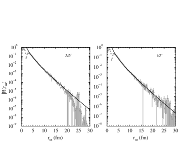
FIG. 1.: Monte Carlo samples of the radial two-cluster $\alpha t$ distribution functions in ⁷Li ground state ($J^{\pi}=3/2^{-}$, left panel) and first excited state ($J^{\pi}=1/2^{-}$, right panel), with error estimates. The solid curve is the expected Whittaker-function asymptotic form of the overlap, normalized as in Table II to match the $\alpha\tau$ distributions at 7–10 fm.

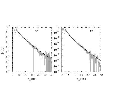
FIG. 2.: Same as Fig. 1, but for radial two-cluster $\alpha^{3}{\rm He}$ distribution functions in ⁷Be bound states.

As noted in the Introduction, low-energy direct captures can be treated to good approximation by considering only cluster separations beyond a few fm, and using only the longer-range parts of the bound- and initial-state wave functions to compute matrix elements. This approach requires the provision of “spectroscopic factors,” or more precisely, the ANCs discussed above. Because we have imposed the condition that the large-cluster-separation part of the ground state match its expected form, it is true that for our cross section calculations, the VMC method provides $C_{1}$. However, it also provides the inner few fm of the wave function, which requires some model of what is going on inside the nuclear interaction radius, and may be important for understanding differences in the logarithmic derivatives of the $S$-factor found in various theoretical studies.

B Scattering states

The initial-state wave functions are taken to be elastic-scattering states of the form

$$|\psi_{\alpha\tau};LSJM\rangle={\cal A}\left\{\phi_{\alpha\tau}^{JL}(r_{\alpha\tau})Y_{LM_{L}}({\bf\hat{r}}_{\alpha\tau})\prod_{ij}G_{ij}|\psi_{\alpha}\psi_{\tau}^{m_{S}}\rangle\right\}_{LSJM},$$ (20)

where curly braces indicate angular momentum coupling, $\cal{A}$ antisymmetrizes between clusters, $\psi_{\alpha}$ is the ⁴He ground state, and $\psi_{\tau}^{m_{S}}$ is the trinucleon ground state in spin orientation $m_{S}$.

The $G_{ij}$ are identity operators if the nucleons $i$ and $j$ are in the same cluster. Otherwise, they are a set of both central and non-central pair correlation operators which introduce distortions in each cluster, under the influence of individual nucleons from the other cluster. They are derived from solutions for nucleon-nucleon correlations in nuclear matter [37], and become the identity operator at pair separations beyond about 2 fm. (These correlations have been included in the definition of the overlap functions shown in Figs. 1 and 2.)

The correlations $\phi_{\alpha\tau}^{JL}$ are derived phenomenologically. The variational seven-body bound-state wave functions do not give the correct energies with respect to cluster breakup, so we do not expect to be able to use the variational technique to solve for these correlations. Instead, we generate the $\phi_{\alpha\tau}^{JL}$ as solutions to Schrödinger equations, from cluster-cluster potentials that describe phase shifts of $\alpha$-${}^{3}{\rm H}$ and $\alpha$-${}^{3}{\rm He}$ scattering as scattering of point particles. Because of the small amount of available laboratory data and the large amount of work that has already been put into generating potentials that reproduce them, we take cluster-cluster potentials from the literature [4, 5, 6, 7, 19]. We now point out the main features of these potentials.

We treat all of these models as (and many have been explicitly constructed as) descriptions of both the $\alpha t$ and $\alpha\,^{3}{\rm He}$ systems, with appropriate Coulomb potentials and laboratory masses. Each of the potentials we use to generate the $\phi_{\alpha\tau}^{JL}$ has a deep, attractive central term, and a spin-orbit term. The spin-orbit terms are constrained mainly by the spacing between the $P_{3/2}$ and $P_{1/2}$ bound states, and between the resonances at 2.16 and 4.21 MeV in $F_{7/2}$ and $F_{5/2}$ $\alpha t$ scattering, respectively (as well as their analogs in $\alpha\,^{3}{\rm He}$ scattering). The other interesting feature in the scattering of the odd partial waves is the apparent hard-sphere behavior of the phase shifts in $P$-wave scattering. This comes about because the wave functions between the clusters must respect the Pauli principle by allowing antisymmetrization of nucleon wave functions between clusters. In the $P$ waves, this takes the form of wave functions that have a single node whose location is almost independent of scattering energy, and it therefore gives rise to phase shifts which look like scattering from a hard sphere [38]. (See Figs. 1 and 2, where the steep dips in absolute values of the cluster distributions at 2 fm correspond to nodes). In the cluster-cluster potentials, this requires that the central term be large and negative, so that the ground state wave function has one node. Of course, a more tightly-bound “forbidden” state with zero nodes exists for such a potential, but it does not allow antisymmetrization of the nucleon wave functions. We note that the requirement of a particular nodal structure only models approximately the effects of the Pauli principle on the inter-cluster correlations. We did not use potentials that enforced the hard-sphere behavior with repulsive short-range terms [39].

Because of the requirements of the Pauli principle, one also expects different potentials to describe the odd- and even-parity scattering. The even-parity phase shifts are unfortunately lacking in details which models must match (see Fig. 3), beyond the apparent hard-sphere scattering in the $S$-wave data, corresponding to the Pauli-required minimum of two nodes in the wave function [38]. The measured $D$-wave phase shifts are even worse, being consistent with zero (or $180^{\circ}$, with the knowledge that there must be at least one node in the wave function) throughout the region below 8 MeV for both $\alpha$-t and $\alpha$-${}^{3}{\rm He}$ systems [40, 41, 42, 43]. This lack of features is particularly unfortunate in that by far the most important reaction mechanisms for radiative capture in this system are $E1$ captures from $S$- and $D$-wave scattering states. The most stringent tests of any of the $D$-wave potentials have been comparison of their phase shifts with the results of more elaborate (RGM) theoretical models.

Finally, we note the difficulty of reproducing the published models, which is due to omitted descriptions of details of the potentials, particularly handling of the Coulomb potential at short range. Rather than guess how to fix up each potential, we restrict attention to potentials that allowed good descriptions of the low-energy scattering on the first try (with no short-range cutoff in the $1/r$ Coulomb term unless explicitly described by the potential’s authors). Relatively small differences in the cluster-cluster potentials are directly connected to the size of the scattering wave function at energies less than 1 MeV and cluster separations less than 20 fm, resulting directly in differences in the normalization of our computed capture cross sections from one potential to the next. However, it is possible to eliminate the worst potentials on the basis of the low-energy phase shifts; potentials which underpredict the phase shifts also produce radiative capture cross sections that are too low by as much as a factor of two, relative to those generated from other cluster-cluster potentials. Potentials which were created for use in orthogonal cluster models (as opposed to simple cluster models) were eliminated from application to our problem on this criterion.

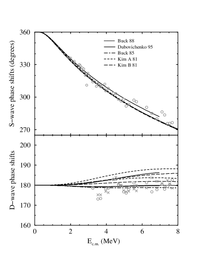
FIG. 3.: Phase shifts produced by the potentials used to generate the $\phi_{\alpha\tau}^{JL}$. Data are taken from Refs. [42, 43]; in the lower panel, $\times$ denotes $J^{\pi}=\frac{5}{2}^{+}$ phase shifts, $\circ$ denotes $J^{\pi}=\frac{3}{2}^{+}$ phase shifts. Potentials are taken from Refs. [4, 5, 6, 7].

III Operators

The cross sections were computed by a multipole expansion of the electromagnetic current operator [44],

$$\sigma(E_{\rm c.m.})=\sum_{LSJ_{i}J_{f}\ell}\frac{8\pi}{2J_{f}+1}\frac{\alpha}{v_{\rm rel}}\frac{q}{1+q/m_{\rm 7}}\Bigg{[}\left|E^{LSJ_{i}J_{f}}_{\ell}(q)\right|^{2}+\left|M^{LSJ_{i}J_{f}}_{\ell}(q)\right|^{2}\Bigg{]}\ ,$$ (21)

where $\alpha$ is the fine structure constant ($\alpha=e^{2}/\hbar c$), $v_{\rm rel}$ is the $\alpha$$\tau$ relative velocity, $m_{7}$ is the mass of the final state, and $E^{LSJ_{i}J_{f}}_{\ell}(q)$ and $M^{LSJ_{i}J_{f}}_{\ell}(q)$ are the reduced matrix elements (RMEs) of the electric and magnetic multipole operators with multipolarity $\ell$ connecting the scattering states in channel $LSJ_{i}$ to bound states of ⁷Li or ⁷Be with angular momentum $J_{f}$. The center-of-mass energy of the emitted photon is given by

$$q = m_{\rm 7}\Bigg{[}-1+\sqrt{1+\frac{2}{m_{7}}(m_{\tau}+m_{\alpha}-m_{7}+E_{\rm c.m.})}\Bigg{]},$$ (22)

$$\simeq m_{\alpha}+m_{\tau}-m_{7}+E_{\rm c.m.}$$ (23)

where $m_{\tau}$, $m_{\alpha}$, and $m_{7}$ are the rest masses of the trinucleon, ⁴He, and the appropriate ⁷Li or ⁷Be state, respectively. The astrophysical $S$-factor is then related to the cross section via

$$S(E_{\rm c.m.})=E_{\rm c.m.}\,\sigma(E_{\rm c.m.})\,{\rm exp}(2Z_{1}Z_{2}\,\pi\,\alpha/\hbar v_{\rm rel})\ ,$$ (24)

where $Z_{1}$ and $Z_{2}$ are the charges of the two initial-state nuclei.

The dominant reaction mechanism, for creation of both the excited state and the ground state, is an $E1$ (electric dipole) transition from an $S$-wave scattering state to a bound state. Capture into the excited state is followed immediately by electromagnetic decay to the ground state, so the total cross section of interest for astrophysics is the sum of the cross sections for captures into the two states. At energies above about 500 keV, $E1$ capture from $D$ waves becomes important. We computed transitions originating from scattering states with orbital angular momentum $L=0,1,2$ and 3, via $M1,M2,E1,E2,$ and $E3$ transitions, and found that up to the 0.1% level, only $E1$ captures originating from $S$- and $D$-wave scattering states matter at energies below 1.5 MeV.

With the exception of the $E1$ term, all RMEs were computed in the standard long-wavelength approximation (LWA), keeping only the lowest-order term in photon wavenumber of the modified spherical Bessel functions appearing in the RME integrals. The LWA is valid to reasonable accuracy because at the low energies under consideration ($E<1$ MeV), the ratio of system size to photon wavelength is less than $10\ {\rm fm}/200\ {\rm fm}=0.05$.

In a previous study [25], we developed code to examine the isospin-forbidden $E1$ transition in $d(\alpha,\gamma)^{6}{\rm Li}$. We have applied this code to compute corrections to the LWA for the $E1$ transitions under consideration here. An examination of these corrections for the mass-seven system is in principle of interest for the problem of extrapolating cross sections to low energies. However, we find that all but one of them provide contributions of less than 0.05% of the total cross section. (See Ref. [25] for a list and detailed discussion of the corrections we applied, which extend to third order in $q$.) We do not actually compute the largest correction, which is the “center-of-energy” correction. This correction arises because potentials and kinetic energies should be included in the definition of the center-of-momentum frame, but have not been[45]. The center-of-energy correction becomes important when the leading order LWA operator vanishes, as in $d(\alpha,\gamma)^{6}{\rm Li}$, but it should amount to only +2.4% of the $E1$ cross section in ${}^{3}{\rm H}(\alpha,\gamma)^{7}{\rm Li}$ and +3.1% of the $E1$ cross section in ${}^{3}{\rm He}(\alpha,\gamma)^{7}{\rm Be}$. We did not compute center-of-energy corrections (or include an estimate of them in the results presented below) because of the extra computation necessary to find energies during the capture calculation. Their omission is not serious because 1) their effect is to change the normalization, not the energy dependence of the $E1$ cross section, 2) our model calculation is only accurate to about 5–10% at best, and 3) the above estimates of the size of the effect should be quite accurate, being based only on the differences between using nuclear masses and using integer multiples of the mean nucleon mass in the factor $[(Z_{2}m_{1}-Z_{1}m_{2})/(m_{1}+m_{2})]^{2}$ in the LWA cross section.

A Matrix element integration

Actual computation of the matrix elements was performed with a modified version of the code described in Ref. [25], which is itself a modified version of a code developed to compute energies and other properties of light nuclei [27] for variational calculations. The method used to integrate over nucleon configurations is the Metropolis Monte Carlo algorithm, with a weight function proportional to the bound state wave function involved in the computed transition. As discussed below, this weight function was chosen to reflect in general detail the form of the matrix element integrands, and to obtain significant numbers of Monte Carlo samples over a broad range of cluster separations. The final calculation consisted of $10^{6}$ samples for each transition.

We have applied the approach of splitting the calculation into energy-dependent and energy-independent parts, as in Ref. [46], so that the reduced matrix elements of Eq. (21) are written

$$T^{LSJ_{i}J_{f}}_{\ell}(q) =\frac{\sqrt{2J_{f}+1}}{<J_{i}M_{i},\ell\lambda|J_{f}m_{f}>}$$ (26)

$$\times\int_{0}^{\infty}dx\,x^{2}\,\phi_{\alpha\tau}^{J_{i}L}(x)\langle\psi_{7}^{J_{f}m_{f}}|T_{\ell\lambda}(q){\cal A}\left\{\delta(x-r_{\alpha\tau})Y_{L}^{M_{L}}({\bf\hat{r}}_{\alpha\tau}))\prod_{ij}G_{ij}|\psi_{\alpha}\psi_{\tau}^{m_{S}}\rangle\right\}_{LSJ_{i}M_{i}}$$

and computed using photon polarization $\lambda=+1$ for the multipole operators $T_{\ell\lambda}(q)$. The delta function is applied by accumulating the Monte Carlo integral in radial bins of thickness $0.25$ fm. The final integration over $x$ is performed by inserting the appropriate dependences on photon energy in each term (since the LWA expansion is in powers of energy, this dependence may be taken out of the integral), and computing $\phi_{\alpha\tau}^{JL}$, at each energy. This allows the time-consuming Monte Carlo integration to be performed only once for each partial wave and operator, so that computation of RMEs for many energies is relatively inexpensive in computer time. After initially setting up the code and checking that selection rules were satisfied, we did not explicitly compute RMEs for parity-forbidden operators.

At cluster separations beyond about 10 fm, the RME densities were subject to considerable noise in the Monte Carlo sampling. This is because while Monte Carlo weighting schemes based on the ground state give good sampling along directions other than the cluster separation in the $3A$-dimensional configuration space, they provide small numbers of samples at large $r_{\alpha\tau}$ (due to exponential decay of the wave function at large distances). VMC work usually uses weighting based on the inner product in spin-isospin space of a simplified bound state with itself. Such weighting is good for minimizing Monte Carlo variance of integrands that resemble the bound state probability density closely, such as energies, but it does not provide enough samples in the asymptotic region of the wave function to do low-energy direct capture calculations. Our previous paper [25] used the square root of the usual weight function, extending the Monte Carlo sampling out to large cluster separations, but at the expense of greater sampling noise for a fixed number of samples at fixed cluster separation. In the mass-six problem, it was straightforward to run the Monte Carlo integration of the RMEs until the densities had “converged” to the expected asymptotic forms at large cluster separation. This required about $2\times 10^{6}$ total configurations for a given RME. At $A=7$, the spin-isospin space is larger, so the code is slower by a factor of about 10, and it was only practical to obtain $10^{6}$ samples for each RME with available computing resources. However, since the configuration space gains three dimensions with the addition of a particle, $10^{6}$ samples do not provide as thorough of a sample of the configuration space at mass 7 as at mass 6. The result is at best a few-percent measure of the asymptotic normalization at 7–10 fm. Many samples are obtained at larger cluster separation with the new weighting scheme, but the samples beyond 15 fm appear to have correlated noise. This is presumably because the samples in question correspond to only a few excursions of the sampling Markov chain into the region of large cluster separation, and are therefore not very independent from each other. They tend to be either mostly high or mostly low relative to the asymptotic forms explicitly built into the wave functions. See Fig. 4 for illustration of these difficulties. A much larger sample (by a factor of 10) would be expected to exhibit much less of this sort of correlated noise, but is prohibited by the large amount of computer time that would require.

The matrix elements were therefore integrated out to 7 fm using the Monte Carlo results for the integrand of Eq. (26); integration beyond 7 fm was carried out using the known asymptotic forms of the matrix element densities, normalized to the Monte Carlo output by least-squares fitting at 7–10 fm. This range was arrived at by comparing results for the ANC of the ⁷Li ground state arising from two different weighting schemes and varying numbers of samples. Reasonably consistent agreement was found by fitting at 7–10 fm in all cases. The accuracy in the cross section then depends on how accurately the ANCs can be determined in this region.

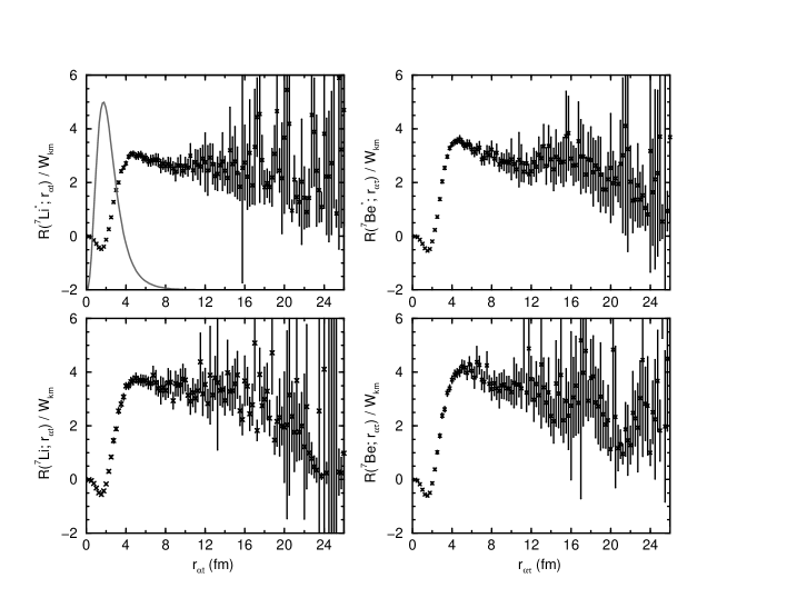
FIG. 4.: Ratios of the computed radial overlap functions of Figs. 1 and 2 to their imposed asymptotic forms, based on $10^{6}$ particle configurations. These ratios should be equal to the asymptotic normalization constant for the appropriate wave function beyond about 7 fm. Superimposed on the ratios for the ⁷Li excited state is the corresponding distribution of Monte Carlo samples, essentially identical for all four overlap functions.

IV Cross sections

A ${}^{3}{\rm H}(\alpha,\gamma)^{7}{\rm Li}$

The computed $S$-factor for ${}^{3}{\rm H}(\alpha,\gamma)^{7}{\rm Li}$ is shown broken down into contributions from various terms of Eq. (21) in Fig. 5, and in comparison with laboratory data in Fig. 6. The dominant processes are obviously $E1$ captures, with large contributions from captures into both the ground and excited states. Contributions from other partial waves and multipole operators are not present above the 1% level. Contributions from higher-order LWA corrections to the $E1$ operator are less than 0.02%. Our calculations are therefore limited in accuracy only by 1) the accuracy of the (bound- and scattering-state) wave functions, and 2) Monte Carlo statistics.

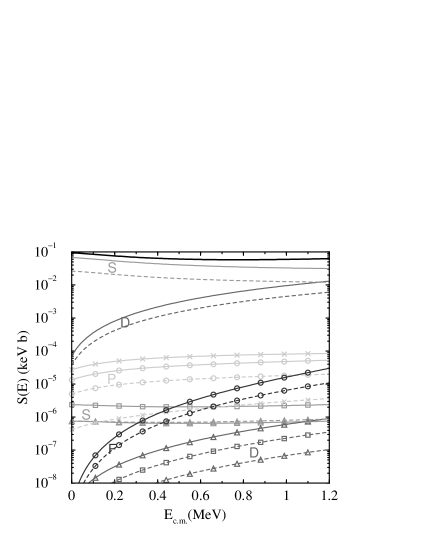
FIG. 5.: Low-energy $S$-factor for ${}^{3}{\rm H}(\alpha,\gamma)^{7}{\rm Li}$ (thick solid line), and its breakdown into contributions from various partial strengths, computed using potential A of Kim et al. [5]. Transitions to the ground state are shown as solid lines, and transitions to the excited state as dashed lines. Labels indicate the initial state, and additional symbols indicate multipole operator: no symbol, $E1$; $\circ$, $E2$; $\times$, $M1$; $\Box$, $M2$; and $\triangle$, order $q^{3}$ spin correction to $E1$ operator (LWA2 of Ref. [25]).

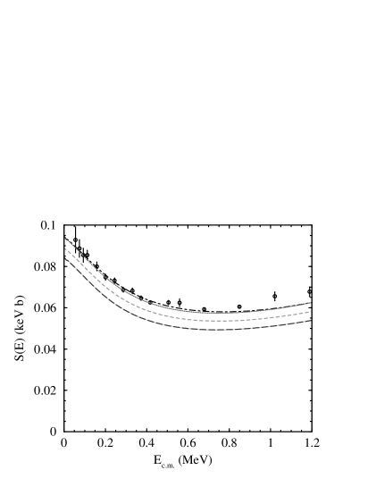
FIG. 6.: Same as Fig. 5, but showing only total $S$-factors for several different potentials used to generate cluster correlation functions $\phi_{\alpha t}^{JL}$: dot-dashed and dotted, potentials A and B respectively of Kim et al.[5]; short-dashed, from Dubovichenko et al.[4], solid, from Buck et al. [6]; and long-dashed, from Buck and Merchant [7]. Data are from Brune et al. [20], and share a common 6% normalization uncertainty, not shown.

The present calculation is the result of sampling $10^{6}$ points in the seven-particle configuration space. Formal error estimation on the resulting cross sections is difficult because all 35 partitions of the seven nucleons into alpha and triton clusters were computed for each configuration. This saves computation time, and enforces antisymmetry of the initial state exactly; it also introduces correlations between values of the operator densities (integrands of Eq. (26)) at different cluster separations. The uncertainties in different transitions and partial waves are also correlated, because they are based on the same random walk of particle configurations. There is also an uncertainty from the wave function normalizations, because they are also derived from Monte Carlo integrations. This last uncertainty amounts to about 3% in the cross section.

We take the best indication of the Monte Carlo uncertainty to be the formal uncertainties on the asymptotic normalizations of the Monte Carlo matrix element densities, which we used to compute matrix element contributions beyond cluster separations of 7 fm. The asymptotic forms of the matrix element densities are the Whittaker-function asymptotic forms discussed above, multiplied by the radial dependences of the electromagnetic multipole operators. The normalizations were fitted to the matrix element densities at cluster separations of 7–10 fm. Using fitted asymptotic forms amounts to treating a large part of the matrix element as an external direct capture, and it fixes two problems. First, it removes the need for large numbers of Monte Carlo samples in the remote tails of the wave function. Second, the asymptotic normalizations are found by a weighted least-squares procedure, and formal error estimates on these normalizations are possible. In practice, the correlations between matrix element densities produce reduced $\chi^{2}$ significantly less than unity. A common approach when confronted with such a problem in experimental data is to assume that uncertainties have been overestimated, and to reduce formal uncertainties accordingly. We have not done this, and we arrive at uncertainties of approximately 10% in the cross section, based on the formal error estimates (corresponding closely to the sizes of ANC errors in Table II). More detailed analysis is problematic, and it is not called for because the 10% estimate is already larger than any other contribution to the error budget.

The results themselves are best characterized in three ways:

1) Normalization. Our results are lower than the data of Brune et al. [20] by 0–20%, depending on the cluster potential. Although other data exist [47, 48, 49, 50, 51], those of Brune et al. are much more precise, and permit the best test of our results. Those data share a common 6% normalization uncertainty, not shown in Fig 6. The systematic discrepancy between some of our results and the data is probably small enough to ascribe to the combined uncertainties of the Monte Carlo integration and of the data. Taking the branching ratio to have its experimental value of $R=0.453$, the computed $S$-factors for transitions to the ground state match the measured low-energy $S$-factors, while those for the excited state do not. The normalization is affected significantly by the choice of potential used to generate the inter-cluster correlations $\phi_{\alpha t}^{JL}$ for the scattering states. By applying five different potentials from the literature as described above, we obtain a variation of $\pm 5\%$ in the $S(0)$ (total range for the five potentials) about a mean of 0.90 keV$\cdot$b – a full range equal in size to the Monte Carlo uncertainty. Summarizing our results in one number, we obtain using the inter-cluster potential A of Kim et al.[5] (the best fit to the $S$-wave phase shifts), $S(0)=0.095$ keV b, similar to other estimates found in the literature.

2) Branching ratio. The branching ratio $R$, defined as the ratio of the cross section for capture into the excited state to that for the ground state, is shown in comparison with the Brune data in Fig. 7. A weighted least-squares normalization of the calculation to the laboratory data shows that our calculation of $R$ is lower than the data by 15%, which can be combined with the results above to infer that the excited-state ANC is low by 8%, within the range of the Monte Carlo sampling error. The energy dependence of the branching ratio matches the data with a $\chi^{2}$ of 26.0 for 15 degrees of freedom, about as well as the straight line fits of Brune et al.

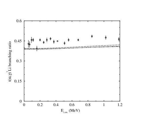
FIG. 7.: Computed ratio of the cross section for capture into the excited state to that for capture into the ground state, for ${}^{3}{\rm H}(\alpha,\gamma)^{7}{\rm Li}$. Symbols are the same as in Fig. 6, and the data share a normalization uncertainty of 4% (not shown).

3) Energy dependence. The energy dependence of the ${}^{3}{\rm H}(\alpha,\gamma)^{7}{\rm Li}$ $S$-factor at low energy is almost completely independent of cluster-cluster potential, for the five potentials examined. After normalizing the computed cross section (with cluster correlations computed from potential A of Kim et al. [5]) to match the Brune data, we obtain a $\chi^{2}$ of 38.7 for 16 degrees of freedom. A significantly better fit results if the highest 3 points in energy (where $D$-wave capture becomes important) are excluded. The residuals of $-1.8\%$ to $+8.5\%$ compare favorably with other theoretical calculations, but the energy dependence of the calculation is systematically shallower than that of the data at the highest-energy points. Our calculation of the $S$ factor gives a logarithmic derivative at $E=0$ of $-0.972\ {\rm MeV}^{-1}$ – about equal to that found by Mohr et al. [8], but half of that found in other theoretical studies [7, 14, 17], and about 2/3 of that suggested in a recent compilation of astrophysical reaction rates [52].

B ${}^{3}{\rm He}(\alpha,\gamma)^{7}{\rm Be}$

The low-energy $S$-factor computed from the Kim A cluster-cluster potential for ${}^{3}{\rm He}(\alpha,\gamma)^{7}{\rm Be}$ is shown in Fig. 8, along with the contributions of individual terms of Eq. (21). Total $S$-factors from five cluster-cluster potentials are shown along with the laboratory data in Fig. 9. The computed branching ratios are shown along with the corresponding data in Fig. 10. The discussions of small contributions to the $S$-factor and of the precision of the results for ${}^{3}{\rm H}(\alpha,\gamma)^{7}{\rm Li}$ above also apply here, again with a Monte Carlo error estimate of about 10% in $S$-factor normalization. We again break down the results for ${}^{3}{\rm He}(\alpha,\gamma)^{7}{\rm Be}$ into normalization, branching ratio, and energy dependence:

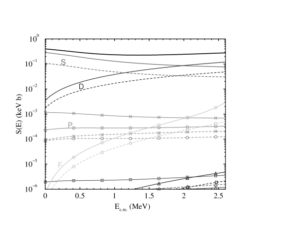
FIG. 8.: Low-energy $S$-factor for ${}^{3}{\rm He}(\alpha,\gamma)^{7}{\rm Be}$ (thick solid line), and its breakdown into contributions from various partial strengths, computed using potential A of Kim et al. [5]. Symbols are as in Fig. 5.

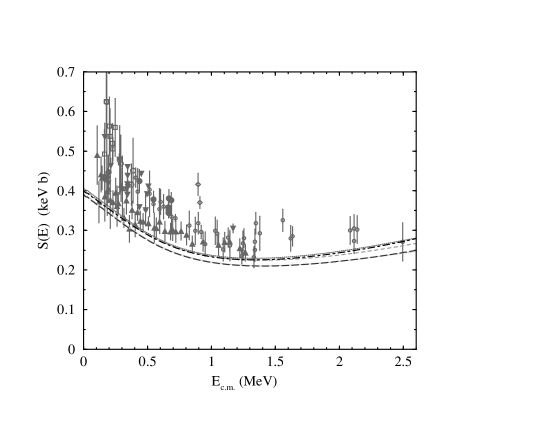
FIG. 9.: Same as Fig. 8, but showing only total $S$-factors for several different potentials used to generate cluster correlation functions $\phi_{\alpha t}^{JL}$, with symbols as in Fig. 6. Data are from Refs. [53, 54, 55, 56, 57, 58]. Symbols for the data are the same as in Ref. [3], with the exception of Refs. [55] ($\Box$) and [57] ($\diamond$) .

1) Normalization. Our $S$-factors are more than 10% lower than the lowest data set (after applying the renormalization of the Kräwinkel data set [54] recommended by Hilgemeier et al. [53]), and nearly a factor of two lower than the highest data sets (note that this includes the data of Volk et al. [59], which are not shown because their results were published only as extrapolated $S(0)$ values). By applying five different phenomenological cluster-cluster potentials that are not in disagreement with the low-energy elastic-scattering data, we obtain a small variation in $S(0)$ about a mean of $S(0)=0.40$ keV b. Using the potential which best matches the low-energy $S$-wave scattering (potential A of Kim et al. [5]), we obtain $S(0)=0.40$ keV b. Although this is closer to matching the lower numbers found in capture photon experiments than the delayed activity experiments, it is not a close match in normalization to any of the experimental results. Our results are therefore not useful for addressing possible systematic problems in the data.

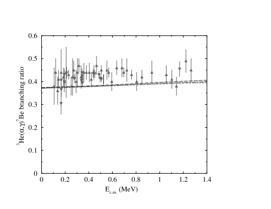
FIG. 10.: Computed ratio of the cross section for capture into the excited state to that for capture into the ground state, for ${}^{3}{\rm He}(\alpha,\gamma)^{7}{\rm Be}$. Symbols are the same as in Fig. 9.

2) Branching ratio. It is seen from the branching ratios in Fig. 10 that our calculation is in reasonable agreement with the laboratory data with regard to relative strengths of transitions to the ground and first excited states of ⁷Be. This suggests that the ANCs of the VMC wave functions for both states are too small, and by about the same factor in each case. Using the results for $S$-factor normalization above, we conclude that this factor is in the range 5–25%.

TABLE III.: Comparison of energy dependence of calculated $S$-factors with laboratory data, after renormalizing the computed $S$-factor to minimize $\chi^{2}$. $\nu$ denotes number of degrees of freedom, and an estimate of systematic normalization uncertainty was subtracted from the error estimates of the points (as discussed in Ref. [1]) before performing this analysis.

Data set	$\chi^{2}/\nu$	$\nu$
Kräwinkel [54]	$0.364$	37
Parker [56]	$0.917$	37
Hilgemeier [53]	$0.698$	8
Nagatani [55]	$0.450$	6

3) Energy dependence. We renormalized our results to best fit each of the larger data sets separately, and computed chi-squared statistics in each case to determine goodness of fit. The results are shown in Table III, and indicate general agreement. For the logarithmic derivative of $S(E)$ at $E=0$, we obtain $-0.57\ {\rm MeV}^{-1}$, in reasonable agreement with other estimates in the literature [7, 14, 17, 52], where published models fall in the range $-0.50$ to $-0.72$. It is about equal to the value presently used in solar neutrino work [3].

V Implications and Applications

We have carried out the first calculation of the low-energy $S$-factors for the processes ${}^{3}{\rm H}(\alpha,\gamma)^{7}{\rm Li}$ and ${}^{3}{\rm He}(\alpha,\gamma)^{7}{\rm Be}$ based on realistic nucleon-nucleon potentials. Seven-body wave functions for these potentials, constructed by the VMC method and constrained to have the correct asymptotic forms, produce $S$-factor energy dependences for the processes ${}^{3}{\rm H}(\alpha,\gamma)^{7}{\rm Li}$ and ${}^{3}{\rm He}(\alpha,\gamma)^{7}{\rm Be}$ which agree reasonably well with experiment.

This work indicates no serious problems in the reaction rates presently used in astrophysical models. In fact, the most important implication of these results for astrophysics is probably that the previous understanding of these reactions remains essentially unchallenged. For example, using the present calculation to extrapolate the Robertson et al. activity measurement [57] of the $S$-factor from 0.9 MeV to 0 MeV, we obtain essentially the same result as with the energy dependence currently used in the standard solar model [3]. For big-bang nucleosynthesis, there is no low-energy extrapolation problem. The most useful result which a theoretical study could provide for cosmology would therefore be tighter constraints on cross-section normalizations than the current body of experimental data provides. The present calculations have not achieved that goal, but future first-principles calculations based on realistic nucleon-nucleon interactions might.

The only serious problem with the results presented here is the low normalization of the $S$-factors, and its principal cause is probably easy to identify. Because most of the cross section arises at large ($>10$ fm) cluster separations, the low normalizations most likely arise from the form of the seven-body bound states at large separations of the p-shell nucleons from the s-shell core. Part of the discrepancy may arise from the correlation $f_{sp}$. The correlation between $\alpha$ and $\tau$ clusters in the bound states is proportional to the twelfth power of $f_{sp}$, so that the long-range correlation between clusters is very sensitive to the choice of $f_{sp}$. However, it is hard to see how the $f_{sp}$ used in this study could affect the wave function beyond about 5 fm cluster separation. In the case of ${}^{3}{\rm H}(\alpha,\gamma)^{7}{\rm Li}$, a more likely explanation is that the Monte Carlo uncertainty has been underestimated, and a (prohibitively) long integration would “converge” on values in better agreement with experiment. Other aspects of the present calculation which are not done as exactly as one may wish, and therefore may bear on this problem, include the fact that asymptotic forms have been imposed on the wave functions which are inconsistent with their energies, as well as the use of cluster-cluster interactions which were phenomenologically constructed and could conceivably be inconsistent with the rest of the calculation in subtle ways.

Despite these lingering difficulties, we have demonstrated the applicability of a new, almost ab initio approach for computing low-energy radiative captures in cases for which precise measurements exist, achieving the same accuracy as previous theoretical approaches. We also have presented additional evidence for uncertainty in the logarithmic derivative of the ${}^{3}{\rm H}(\alpha,\gamma)^{7}{\rm Li}$ $S$-factor at zero energy.

Regarding the present calculation as a first application of realistic potentials to radiative capture at mass seven, it has been successful, and it has taught important lessons about the role of the $f_{sp}$ correlations that were not apparent in previous VMC studies. This work clears the way for more refined models of these radiative captures based on realistic potentials. Specific improvements which will be possible in the near future include the use of improved three-body potentials now in development [32] and the use of essentially exact wave functions derived by the Green’s function Monte Carlo technique for the seven-body bound states. We note that the application of GFMC will require new wave functions, starting from VMC wave functions of the type used here to get the asymptotic forms correct. In the more distant future, it should be possible to perform the whole calculation self-consistently, constructing scattering wave functions from the potentials in a way similar to that used for the bound-state wave functions. VMC-based work would also profit by a more systematic effort to produce a Monte Carlo weighting scheme well-suited to computing the sorts of matrix elements encounted in direct capture calculations. Prospects for significant improvement on this initial investigation are very good.

- [1] K. M. Nollett and S. Burles, Phys. Rev. D 62, 123505 (2000).
- [2] S. Burles, K. M. Nollett, J. W. Truran, and M. S. Turner, Phys. Rev. Lett. 82, 4176 (1999).
- [3] E. G. Adelberger et al., Rev. Mod. Phys. 70, 1265 (1998).
- [4] S. B. Dubovichenko and A. V. Dzhazairov-Kakhramanov, Phys. Atomic Nucl. 58, 579 (1995).
- [5] B. T. Kim, T. Izumoto, and K. Nagatani, Phys. Rev. C 23, 33 (1981).
- [6] B. Buck, R. A. Baldock, and J. A. Rubio, J. Phys. G 11, L11 (1985).
- [7] B. Buck and A. C. Merchant, J. Phys. G 14, L211 (1988).
- [8] P. Mohr, H. Abele, R. Zwiebel, G. Staudt, H. Krauss, H. Oberhummer, A. Denker, J. W. Hammer, and G. Wolf, Phys. Rev. C 48, 1420 (1993).
- [9] H. Walliser, Q. K. K. Liu, H. Kanada, and Y. C. Tang, Phys. Rev. C 28, 57 (1983).
- [10] T. Kajino and A. Arima, Phys. Rev. Lett. 52, 739 (1984).
- [11] H. Walliser, H. Kanada, and Y. C. Tang, Nucl. Phys. A419, 133 (1984).
- [12] Q. K. K. Liu, H. Kanada, and Y. C. Tang, Phys. Rev. C 23, 645 (1981).
- [13] Y. Fujiwara and Y. C. Tang, Phys. Rev. C 28, 1869 (1983).
- [14] T. Kajino, Nucl. Phys. A460, 559 (1986).
- [15] T. Mertelmeier and H. M. Hoffmann, Nucl. Phys. A459, 387 (1986).
- [16] T. Altmeyer, E. Kolbe, T. Warmann, K. Langanke, and H. J. Assenbaum, Z. Phys. A 330, 277 (1988).
- [17] A. Csótó and K. Langanke, Few-Body Systems 29, 121 (2000).
- [18] H. Friedrich, Nucl. Phys. A294, 81 (1978).
- [19] K. Langanke, Nucl. Phys. A 457, 351 (1986).
- [20] C. R. Brune, R. W. Kavanagh, and C. Rolfs, Phys. Rev. C 50, 2205 (1994).
- [21] R. F. Christy and I. Duck, Nucl. Phys. 24, 89 (1961).
- [22] R. B. Wiringa, V. G. J. Stoks, and R. Schiavilla, Phys. Rev. C 51, 38 (1995).
- [23] B. S. Pudliner, V. R. Pandharipande, J. Carlson, and R. B. Wiringa, Phys. Rev. Lett. 74, 4396 (1995).
- [24] R. B. Wiringa, S. C. Pieper, J. Carlson, and V. R. Pandharipande, Phys. Rev. C 62, 014001 (2000).
- [25] K. M. Nollett, R. B. Wiringa, and R. Schiavilla, Phys. Rev. C 63, 024003 (2000).
- [26] R. B. Wiringa, Phys. Rev. C 43, 1585 (1991).
- [27] B. S. Pudliner, V. R. Pandharipande, J. Carlson, S. C. Pieper, and R. B. Wiringa, Phys. Rev. C 56, 1720 (1997).
- [28] A. Arriaga, V. R. Pandharipande, and R. B. Wiringa, Phys. Rev. C 52, 2362 (2000).
- [29] R. B. Wiringa, S. C. Pieper, J. Carlson, and V. R. Pandharipande, Phys. Rev. C 62, 014001 (2000).
- [30] R. B. Wiringa and R. Schiavilla, Phys. Rev. Lett. 81, 4317 (1998).
- [31] S. C. Pieper, private communication.
- [32] S. C. Pieper, V. R. Pandharipande, R. B. Wiringa, and J. Carlson, nucl-th/0102004, submitted to Phys. Rev. C.
- [33] A. Csótó and K. Langanke, Nucl. Phys. A636, 240 (1998).
- [34] J. L. Forest, V. R. Pandharipande, S. C. Pieper, R. B. Wiringa, R. Schiavilla, and A. Arriaga, Phys. Rev. C 54, 646 (1996).
- [35] C. R. Brune, W. H. Geist, R. W. Kavanagh, and K. D. Veal, Phys. Rev. Lett. 83, 4025 (1999).
- [36] S. B. Igamov, R. M. Tursunmuratov, and R. Yarmukhamedov, Phys. At. Nucl. 60, 1126 (1997), [Yad. Fiz. 60, 1252 (1997)].
- [37] I. E. Lagaris and V. R. Pandharipande, Nucl. Phys. A359, 349 (1981).
- [38] D. A. Zaikin, Nucl. Phys. A170, 584 (1971).
- [39] N. B. Shul’gina, B. V. Danilin, V. D. Efros, J. M. Bang, J. S. Vaagen, and M. V. Zhukov, Nucl. Phys. A597, 197 (1996).
- [40] R. J. Spiger and T. A. Tombrello, Phys. Rev. 163, 964 (1967).
- [41] M. Ivanovich, P. G. Young, and G. G. Ohlsen, Nucl. Phys. A110, 441 (1968).
- [42] W. R. Boykin, S. D. Baker, and D. M. Hardy, Nucl. Phys. A195, 241 (1972).
- [43] D. M. Hardy, R. J. Spiger, S. D. Baker, Y. S. Chen, and T. A. Tombrello, Nucl. Phys. A195, 250 (1972).
- [44] J. Carlson and R. Schiavilla, Rev. Mod. Phys. 70, 743 (1998).
- [45] J. L. Forest, V. R. Pandharipande, and J. L. Friar, Phys. Rev. C 52, 568 (1995).
- [46] A. Arriaga, V. R. Pandharipande, and R. Schiavilla, Phys. Rev. C 43, 983 (1991).
- [47] H. D. Holmgren and R. L. Johnston, Phys. Rev. 113, 1556 (1959).
- [48] U. Schröder, A. Redder, C. Rolfs, R. E. Azuma, L. Buchmann, C. Campbell, J. D. King, and T. R. Donoghue, Phys. Lett. B 192, 55 (1987).
- [49] G. M. Griffiths, R. A. Morrow, P. J. Riley, and J. B. Warren, Can. J. Phys. 39, 1397 (1961).
- [50] S. Burzyński, K. Czerski, A. Marcinkowski, and P. Zupranski, Nucl. Phys. A473, 179 (1987).
- [51] H. Utsunomiya et al., Phys. Rev. Lett. 65, 847 (1990).
- [52] C. Angulo et al., Nucl. Phys. A656, 3 (1999).
- [53] M. Hilgemeier, H. W. Becker, C. Rolfs, H. P. Trautvetter, and J. W. Hammer, Z. Phys. A329, 243 (1988).
- [54] H. Kräwinkel et al., Z. Phys. A304, 307 (1982).
- [55] K. Nagatani, M. R. Dwarakanath, and D. Ashery, Nucl. Phys. A128, 325 (1969).
- [56] P. D. Parker and R. W. Kavanagh, Phys. Rev. 131, 2578 (1963).
- [57] R. G. H. Robertson, P. Dyer, T. J. Bowles, C. J. Maggiore, and S. M. Austin, Phys. Rev. C 27, 11 (1983).
- [58] J. L. Osborne, C. A. Barnes, R. W. Kavanagh, R. M. Kremer, G. J. Mathews, J. L. Zyskind, P. D. Parker, and A. J. Howard, Nucl. Phys. A419, 115 (1984).
- [59] H. Volk, H. Kräwinkel, R. Santo, and L. Wallek, Z. Phys. A310, 91 (1983).