Structure functions
for the
three nucleon system

Abstract

The spectral functions and light-cone momentum distributions of protons and neutrons in ³He and ³H are given in terms of the three-nucleon wave function for realistic nucleon-nucleon interactions. To reduce computational complexity, separable expansions are employed for the nucleon-nucleon potentials. The results for the light-cone momentum distributions suggest that they are not very sensitive to the details of the two-body interaction, as long as it has reasonable short-range repulsion. The unpolarised and polarised structure functions are examined for both ³He and ³H in order to test the usefulness of ³He as a neutron target. It is found that the measurement of the spin structure function of polarised ³H would provide a very clear test of the predicted change in the polarised parton distributions of a bound proton.

I Introduction

It is well known that a polarised ³He target can be used as a polarised neutron target. The question we would like to address is how good a polarised neutron target it is for the determination of the neutron spin structure function, $g_{1}$, in deep inelastic scattering. There are two questions that play a central role in resolving this problem. The first is the sensitivity of the light-front momentum distribution to the three-nucleon wave function. For this we need to calculate the spectral function for realistic tri-nucleon wave functions. The second question is a consequence of the fact that the neutron structure function is small in comparison with the proton structure function. This raises the question of the accuracy with which one can extract the polarised neutron structure function from ³He.

To examine these questions we need first to calculate the three-nucleon wave function for a “realistic” nucleon-nucleon potential. To simplify the problem computationally, we consider a separable expansion [1] of the Paris potential (which we call PEST) [2], that gives the same three-nucleon observables as the the original Paris potential in a full multi-channel Faddeev calculation [3, 4]. For comparison we consider two other classes of potentials. The first is a rank one unitary pole approximation (UPA) [5] to the Reid Soft core potential [6]. This has the property that it reproduces the position and residue of the poles in the ¹S₀ and ³S₁-³D₁ channels – i.e., it reproduces the original potential’s deuteron wave function. As a result, it incorporates the short range behaviour of the original interaction. The second is a Yamaguchi type potential with a $D$-state probability of 4% and 7% [7]. These potentials do not include the short range repulsion that is commonly present in nucleon-nucleon interactions.

In Sec. 2, we present the procedure used to determine the three-nucleon wave functions for these potentials, as well as the corresponding three nucleon observables. By comparing the results for these three classes of potential, we are able to determine the importance of short range correlations and the contribution of higher partial waves to the neutron and proton spectral functions and therefore to the light-cone momentum distributions. Since we will be considering both ³He and ³H, we have chosen to work in an isospin basis and therefore neglect the contribution of the Coulomb interaction to the ³He wave function. We do, however, estimate the effect of neglecting the Coulomb correction on the momentum distribution and therefore the structure functions.

In order to analyse the deep inelastic structure functions of $A=3$ nuclei, we need to determine the neutron and proton spectral functions. This is detailed in Sec. 3. Here we compare the results for various two-body potentials, finding that the light-cone momentum distribution is not sensitive to the details of our three-nucleon wave function. In Sec. 4 we turn to the structure functions and examine the ratio of the structure function in the three-nucleon system to that in the deuteron (the EMC effect) for the different interactions. We also examine the possible implication of neglecting the Coulomb interaction in ³He. This opens the way for us to study the sensitivity of the unpolarised and polarised structure functions to the quark distributions in the proton and neutron and the possibility of extracting the neutron spin structure function from polarised ³He data. Finally, in Sec. 4 we present some concluding remarks.

II The three nucleon wave function

For the three-nucleon problem we can determine the non-relativistic wave function by solving the Faddeev equations exactly for any realistic two-body interaction. However, to simplify the computational aspects of the problem, with no sacrifice in the quality of the wave function, we turn to separable expansions that have been extensively tested [3, 4]. This will result in a three-nucleon wave function that can be used to calculate the spectral function and the light-cone momentum distribution. In the present section we detail the three-nucleon formalism required to evaluate the wave functions for ³He and ³H.

A Notation

With the extensive literature on the Faddeev equations[8] and their use in the three-nucleon system, we restrict ourselves here to a summary of the notation used in the present analysis. The Faddeev decomposition of the three-nucleon wave function is given by

$$\left|\Psi\right\rangle=\left|\varphi_{1}\right\rangle+\left|\varphi_{2}\right\rangle+\left|\varphi_{3}\right\rangle=\{e+(123)+(132)\}\left|\varphi_{3}\right\rangle\ .$$ (1)

Here “$e$”, “$(123)$” and “$(132)$” are members of the permutation group of three objects, with $e$ being the unit element (i.e. $e\left|\varphi_{\alpha}\right\rangle=\left|\varphi_{\alpha}\right\rangle$) and the other two being cyclic permutations of $\{1,2,3\}$. The second equality results from the requirement that we have identical particles, the wave function is then invariant under any cyclic permutation of our particles. Since we have a system of identical fermions, the total wave function must be antisymmetric under the exchange of any two particles in the system. This requirement leads to following conditions

$$(\alpha\beta)\left|\varphi_{\alpha}\right\rangle = -\left|\varphi_{\beta}\right\rangle,$$ (2)

$$(\alpha\beta)\left|\varphi_{\beta}\right\rangle = -\left|\varphi_{\alpha}\right\rangle,$$ (3)

$$(\alpha\beta)\left|\varphi_{\gamma}\right\rangle = -\left|\varphi_{\gamma}\right\rangle\ .$$ (4)

In the above equations $\alpha$, $\beta$ and $\gamma$ are indices running from 1 to 3, and always different from each other, and $(\alpha\beta)$ is again a member of the permutation group of three objects which exchange particles $\alpha$ and $\beta$ leaving the third one unchanged. Since we are dealing with a three-body problem, there will be only two independent momenta in the centre of mass frame. All the particles have spin and isospin $\frac{1}{2}$ and one must account for their orbital angular momentum. We briefly summarise the quantum numbers and momenta used throughout this paper:

• $N_{\alpha}$ is a set of quantum numbers describing a three body channel from the point of view of the particle $\alpha$, which is the spectator; the set is unique for each channel.

• $\vec{\ell}_{\alpha}$ is the orbital angular momentum between particles $\beta$ and $\gamma$.

• $\vec{L}_{\alpha}$ is the orbital angular momentum between particle $\alpha$ and the centre of mass of the system consisting of particles $\beta$ and $\gamma$.

• $\vec{\jmath}_{\alpha}$, $\vec{\jmath}_{\beta}$, $\vec{\jmath}_{\gamma}$ are the spins of each particle.

• $\vec{\imath}_{\alpha}$, $\vec{\imath}_{\beta}$, $\vec{\imath}_{\gamma}$ are the isospins of each particle.

• $\vec{p}_{\alpha}$ is the momentum of particle $\alpha$ in the centre of mass frame.

• $\vec{q}_{\alpha}$ is the relative momentum of the pair of particles $\beta$ and $\gamma$, defined as $\vec{q}_{\alpha}=(\vec{p}_{\gamma}-\vec{p}_{\beta})/2$.

• $\vec{I}$ and $\vec{J}$ are respectively the total isospin and total angular momentum of the system.

B The partial wave expansion

We now turn to the partial wave expansion of our wave function. To minimise the number of coupled Faddeev equations, having truncated the interaction to a set of partial waves, we have used the following coupling scheme:

$$\vec{\jmath}_{\beta}+\vec{\jmath}_{\gamma}=\vec{s}_{\alpha}, \;\vec{\ell}_{\alpha}+\vec{s}_{\alpha}=\vec{\bar{\jmath}}_{\alpha}, \;\vec{\bar{\jmath}}_{\alpha}+\vec{\jmath}_{\alpha}=\vec{S}_{\alpha},\;\vec{L}_{\alpha}+\vec{S}_{\alpha}=\vec{J},$$

$$\vec{\imath}_{\beta}+\vec{\imath}_{\gamma}=\vec{\bar{\imath}}_{\alpha}, \vec{\bar{\imath}}_{\alpha}+\vec{\imath}_{\alpha}=\vec{I}\ ,$$

which is known as the channel coupling scheme. With this coupling scheme the complete set of quantum number $N_{\alpha}$ describing a three body channel is; $N_{\alpha}=\{\bar{\imath}_{\alpha},s_{\alpha},\bar{\jmath}_{\alpha},S_{\alpha},L_{\alpha}\}$. A subset of these quantum number that describe the two-body channels is; $n_{\alpha}=\{\bar{\imath}_{\alpha},s_{\alpha},\bar{\jmath}_{\alpha}\}$, and therefore $N_{\alpha}=\{n_{\alpha},S_{\alpha},L_{\alpha}\}$. We have not included $\ell_{\alpha}$ in the set of quantum numbers since the tensor force mixes values of $\ell_{\alpha}$. This allows us to define the angular momentum and isospin basis as

$$\left|\Omega_{\ell_{\alpha}N_{\alpha}}^{JI}\right\rangle=\left|\{L_{\alpha},\,[(\ell_{\alpha},\,(\,\jmath_{\beta},\,\jmath_{\gamma})\,s_{\alpha})\,\bar{\jmath}_{\alpha},\,\jmath_{\alpha}]\,S_{\alpha}\}\,J\right\rangle\ \left|[(\,\imath_{\beta},\,\imath_{\gamma})\,\bar{\imath}_{\alpha},\,\imath_{\alpha}]\,I\right\rangle\ ,$$ (5)

These basis states satisfy the following orthogonality relation $\left\langle\Omega_{\ell_{\alpha}N_{\alpha}}^{JI}\Big{|}\Omega_{\ell_{\beta}N_{\beta}}^{JI}\right\rangle=\delta_{\ell_{\alpha},\ell_{\beta}}\,\delta_{{}_{N_{\alpha},N_{\beta}}}$.

We are now in a position to write the partial wave expansion of the total three-nucleon wave function as

$$\left|\Psi\right\rangle=\sum_{\ell_{\alpha}N_{\alpha}}\left|\Omega_{\ell_{\alpha}N_{\alpha}}^{JI}\right\rangle\ \left|{\cal U}_{\ell_{\alpha}N_{\alpha}}^{IJ}\right\rangle\ ,$$ (6)

where $\left|{\cal U}_{\ell_{\alpha}N_{\alpha}}^{IJ}\right\rangle$ is defined as the radial part of the wave function corresponding to the partial wave $\{\ell_{\alpha},N_{\alpha}\}$.

C Separable potential

To reduce the dimensionality of the Faddeev integral equations from two to one, and in this way simplify the three-body wave function, we have employed a separable expansion of the nucleon-nucleon interaction. Our potential for the interaction of particles $\beta$ and $\gamma$ in a given partial wave is of the form[5]

$$V^{n_{\alpha}}_{\ell_{\alpha},\ell^{\prime}_{\alpha}}=\left|g^{n_{\alpha}}_{\ell_{\alpha}}\right\rangle\lambda^{n_{\alpha}}_{\ell_{\alpha}\ell^{\prime}_{\alpha}}\left\langle g^{n_{\alpha}}_{\ell^{\prime}_{\alpha}}\right|\ ,$$ (7)

where $\left|g^{n_{\alpha}}_{\ell_{\alpha}}\right\rangle$ is a “form factor” and $\lambda^{n_{\alpha}}_{\ell_{\alpha}\ell^{\prime}_{\alpha}}$ is the strength of the potential in that partial wave. By taking $\ell_{\alpha}\neq\ell^{\prime}_{\alpha}$ we can accommodate a tensor interaction, as in the case of the ³S₁-³D₁ nucleon-nucleon channel. The above expression for the potential is for a rank one potential. To incorporate higher rank potentials, we turn the strength $\lambda^{n_{\alpha}}_{\ell_{\alpha}\ell^{\prime}_{\alpha}}$ into a matrix and as a result $\left|g^{n_{\alpha}}_{\ell_{\alpha}}\right\rangle$ is a row matrix. In resorting to separable expansions, we have taken the view that the expansion is a numerical procedure analogous to the use of quadratures. However, a low order expansion, such as the UPA or the use of a separable potential, is justified on the grounds that it generates the same analytic structure in the amplitude (i.e., bound or anti-bound state poles) as a corresponding realistic potential.[9] The use of a separable potential gives rise to a separable $t$-matrix that satisfies the Lippmann-Schwinger (LS) equation;

$$t_{\alpha}(E)=V_{\alpha}+V_{\alpha}\,G_{0}(E)\,t_{\alpha}(E)=(1-G_{0}(E)\,V_{\alpha})^{-1}\ V_{\alpha}\ ,$$ (8)

with $G_{0}(E)=(E-H_{0})^{-1}$ the two-body Green’s function. It is simple to show that the separable $t$-matrix in a given partial wave, resulting from a solution of the LS equation, is of the form

$$t^{n_{\alpha}}_{\ell_{\alpha},\ell^{\prime}_{\alpha}}(E)=\left|g^{n_{\alpha}}_{\ell_{\alpha}}\right\rangle\tau^{n_{\alpha}}_{\ell_{\alpha}\ell^{\prime}_{\alpha}}(E)\left\langle g^{n_{\alpha}}_{\ell^{\prime}_{\alpha}}\right|\ ,$$ (9)

where the form factor $\left|g^{n_{\alpha}}_{\ell_{\alpha}}\right\rangle$ is identical to that used in the separable potential. The function $\tau^{n_{\alpha}}_{\ell_{\alpha}\ell^{\prime}_{\alpha}}(E)$, in a given channel, can be a written in matrix form as

$$\left[\tau^{n_{\alpha}}(E)\right]^{-1}=[\lambda^{n_{\alpha}}]^{-1}-\left\langle g^{n_{\alpha}}\left|\,G_{0}(E)\,\right|g^{n_{\alpha}}\right\rangle\ .$$ (10)

This separability of the $t$-matrix will allow us to reduce the dimensionality of the Faddeev integral equations from two to one after the partial wave expansion described in Eq. (6).

D The three-nucleon wave function

Having determined the structure of the two-body amplitude, we now turn to the wave function for the three-nucleon system. The Schrödinger equation for this system is

$$(E-H_{0})\left|\Psi\right\rangle=V\left|\Psi\right\rangle=\sum^{3}_{\alpha=1}V_{\alpha}\left|\Psi\right\rangle\ .$$ (11)

This can be rewritten in a form that suggests the Faddeev decomposition stated in Eq. (1), i.e.,

$$\left|\Psi\right\rangle=G_{0}(E)\,V\left|\Psi\right\rangle=\sum^{3}_{\alpha=1}G_{0}(E)\,V_{\alpha}\left|\Psi\right\rangle=\sum^{3}_{\alpha=1}\left|\varphi_{\alpha}\right\rangle\ .$$ (12)

Here, $G_{0}(E)=(E-H_{0})^{-1}$ is the three-body Green’s function. We now can write an equation for the Faddeev components of the wave function as

$$\left|\varphi_{\alpha}\right\rangle=G_{0}(E)\,V_{\alpha}\left|\Psi\right\rangle=G_{0}(E)\,V_{\alpha}\left|\varphi_{\alpha}\right\rangle+\sum_{\gamma\neq\alpha}G_{0}(E)\,V_{\alpha}\left|\varphi_{\gamma}\right\rangle\ .$$ (13)

With the help of Eq. (8), the set of coupled integral equations for the Faddeev components of the wave function, $\left|\varphi_{\alpha}\right\rangle$, becomes

$$\left|\varphi_{\alpha}\right\rangle=G_{0}(E)\,T_{\alpha}(E)\left(\left|\varphi_{\beta}\right\rangle+\left|\varphi_{\gamma}\right\rangle\right)\ .$$ (14)

Here $T_{\alpha}(E)$ is the $t$-matrix for particles $\beta$ and $\gamma$ in the three-particle Hilbert space, which is related to the two-body amplitude considered in the last section by

$$T_{\alpha}(E)=t_{\alpha}(E-\epsilon_{\alpha})\ ,$$ (15)

where $\epsilon_{\alpha}$ is the energy of the spectator particle $\alpha$ in the three-body centre of mass.

In Eq. (14) we have a set of coupled integral equations, known as the Faddeev equations, for the three-body bound state. For the three-nucleon system, where we have identical Fermions, we take advantage of the anti-symmetry, as given in Eq. (3), and the fact that $(\beta\gamma)T_{\alpha}=T_{\alpha}(\beta\gamma)=-T_{\alpha}$, to reduce the Faddeev equations to

$$\left|\varphi_{\alpha}\right\rangle=G_{0}(E)\,T_{\alpha}(E)\,\left(1-(\beta\gamma)\right)\left|\varphi_{\beta}\right\rangle=2\,G_{0}(E)\,T_{\alpha}(E)\left|\varphi_{\beta}\right\rangle\ ,$$ (16)

with $\alpha\neq\beta$. To recast this equation into a form that will admit numerical solutions, we need to first partial wave decompose the Faddeev equations and take into consideration the separability of the two-body amplitudes. This can all be achieved by partial wave expanding the two-body amplitude in three-body Hilbert space in terms of the angular momentum states defined in Eq. (5) [10]

$$T_{\alpha}(E) = \sum_{\ell_{\alpha}\ell^{\prime}_{\alpha}\atop N_{\alpha}JI}\int\limits_{0}^{\infty}dp_{\alpha}\,p_{\alpha}^{2}\ \left|\Omega^{JI}_{\ell_{\alpha}N_{\alpha}};p_{\alpha}\left\rangle\ t^{n_{\alpha}}_{\ell_{\alpha}\ell^{\prime}_{\alpha}}(E-\epsilon_{\alpha})\ \right\langle p_{\alpha};\Omega^{JI}_{\ell^{\prime}_{\alpha}N_{\alpha}}\right|$$ (17)

$$= \sum_{\ell_{\alpha}\ell^{\prime}_{\alpha}\atop N_{\alpha}JI}\int\limits_{0}^{\infty}dp_{\alpha}\,p_{\alpha}^{2}\ \left|\Omega^{JI}_{\ell_{\alpha}N_{\alpha}};g^{n_{\alpha}}_{\ell_{\alpha}}\left\rangle\ \tau^{n_{\alpha}}_{\ell_{\alpha}\ell^{\prime}_{\alpha}}(E-\epsilon_{\alpha})\ \right\langle g^{n_{\alpha}}_{\ell^{\prime}_{\alpha}};\Omega^{JI}_{\ell^{\prime}_{\alpha}N_{\alpha}}\right|$$ (18)

where $\epsilon_{\alpha}=\frac{3}{4m}p^{2}_{\alpha}$ and

$$\left|\Omega^{JI}_{\ell_{\alpha}N_{\alpha}};g^{n_{\alpha}}_{\ell_{\alpha}}\right\rangle\ =\left|\Omega^{JI}_{\ell_{\alpha}N_{\alpha}}\right\rangle\ \left|g^{n_{\alpha}}_{\ell_{\alpha}};p_{\alpha}\right\rangle\ .$$ (19)

We now can write Eq. (16) as

$$\left|\varphi_{\alpha}\right\rangle = 2\,G_{0}(E)\,\sum_{\ell_{\alpha}\ell^{\prime}_{\alpha}\atop N_{\alpha}JI}\int\limits_{0}^{\infty}dp_{\alpha}\,p_{\alpha}^{2}\ \left|\Omega^{JI}_{\ell_{\alpha}N_{\alpha}};g^{n_{\alpha}}_{\ell_{\alpha}}\right\rangle\ \tau^{n_{\alpha}}_{\ell_{\alpha}\ell^{\prime}_{\alpha}}(E-\epsilon_{\alpha})\ \left\langle g^{n_{\alpha}}_{\ell^{\prime}_{\alpha}};\Omega^{JI}_{\ell^{\prime}_{\alpha}N_{\alpha}}\Big{|}\varphi_{\beta}\right\rangle$$ (20)

$$\equiv 2\,G_{0}(E)\,\sum_{\ell_{\alpha}\ell^{\prime}_{\alpha}\atop N_{\alpha}JI}\int\limits_{0}^{\infty}dp_{\alpha}\,p_{\alpha}^{2}\ \left|\Omega^{JI}_{\ell_{\alpha}N_{\alpha}};g^{n_{\alpha}}_{\ell_{\alpha}}\right\rangle\ \tau^{n_{\alpha}}_{\ell_{\alpha}\ell^{\prime}_{\alpha}}(E-\epsilon_{\alpha})\ X^{JI}_{N_{\alpha}\ell^{\prime}_{\alpha}}(p_{\alpha})\ ,$$ (21)

with the spectator function, $X^{JI}_{N_{\alpha}\ell_{\alpha}}(p_{\alpha})$, satisfying the equation

$$X^{JI}_{N_{\alpha}\ell_{\alpha}}(p_{\alpha}) \equiv \left\langle g^{n_{\alpha}}_{\ell_{\alpha}};\Omega^{JI}_{\ell_{\alpha}N_{\alpha}}\Big{|}\varphi_{\beta}\right\rangle$$ (22)

$$= 2\,\sum_{\ell_{\beta}\ell^{\prime}_{\beta}\atop N_{\beta}}\int\limits_{0}^{\infty}dp_{\beta}\,p_{\beta}^{2}\ Z^{JI}_{\ell_{\alpha}N_{\alpha};\ell_{\beta}N_{\beta}}(p_{\alpha},p_{\beta};E)$$ (24)

$$\qquad\qquad\qquad\times\tau^{n_{\beta}}_{\ell_{\beta}\ell^{\prime}_{\beta}}(E-\epsilon_{\beta})\ X^{JI}_{N_{\beta}\ell^{\prime}_{\beta}}(p_{\beta})\ ,$$

where

$$Z^{JI}_{\ell_{\alpha}N_{\alpha};\ell_{\beta}N_{\beta}}(p_{\alpha},p_{\beta};E)\equiv\left\langle g^{n_{\alpha}}_{\ell_{\alpha}};\Omega^{JI}_{\ell_{\alpha}N_{\alpha}}\right|\,G_{0}(E)\left|\Omega^{JI}_{\ell_{\beta}N_{\beta}};g^{n_{\beta}}_{\ell_{\beta}}\right\rangle\ ,$$ (25)

with $\alpha\neq\beta$. In Appendix A we give an explicit expression for $Z^{JI}_{\ell_{\alpha}N_{\alpha};\ell_{\beta}N_{\beta}}$, for the coupling scheme used in the present analysis [8, 10]. In Eq. (24) we have a set of coupled, homogeneous, integral equations for the spectator wave function, $X^{JI}_{N_{\alpha}\ell_{\alpha}}(p_{\alpha})$, which we can use to construct the total wave function. Here, we note that the spectator wave function is only a function of the momentum of the spectator particle and the energy of the system, which is the binding energy of ³He or ³H. We now turn to the total wave function for the three-nucleon system. Making use of the orthogonality of the angular functions, $\left|\Omega^{JI}_{\ell_{\alpha}N_{\alpha}}\right\rangle$, we can write the total radial wave function, defined in Eq. (6), as

$$\left|{\cal U}^{JI}_{N_{\alpha}\ell_{\alpha}}\right\rangle = \left\langle\Omega^{JI}_{\ell_{\alpha}N_{\alpha}}\Big{|}\Psi\right\rangle$$ (26)

$$= \left\langle\Omega^{JI}_{\ell_{\alpha},N_{\alpha}}\Big{|}\varphi_{\alpha}\right\rangle+\left\langle\Omega^{JI}_{\ell_{\alpha}N_{\alpha}}\Big{|}\varphi_{\beta}+\varphi_{\gamma}\right\rangle$$ (27)

$$= \left|\eta^{JI1}_{\ell_{\alpha}N_{\alpha}}\right\rangle+\left|\eta^{JI2}_{\ell_{\alpha}N_{\alpha}}\right\rangle\ ,$$ (28)

where

$$\eta^{JI1}_{\ell_{\alpha}N_{\alpha}}(p_{\alpha},q_{\alpha}) \equiv \left\langle p_{\alpha}q_{\alpha}\Big{|}\eta^{JI1}_{\ell_{\alpha}N_{\alpha}}\right\rangle$$ (29)

$$= \left\langle p_{\alpha}q_{\alpha};\Omega^{JI}_{\ell_{\alpha}N_{\alpha}}\Big{|}\varphi_{\alpha}\right\rangle$$ (30)

$$= 2G_{0}(q_{\alpha},p_{\alpha};E)\,g^{n_{\alpha}}_{\ell_{\alpha}}(q_{\alpha})\sum_{\ell_{\alpha}^{\prime}}\tau^{n_{\alpha}}_{\ell_{\alpha}\ell^{\prime}_{\alpha}}(E-\epsilon_{\alpha})X^{JI}_{N_{\alpha}\ell^{\prime}_{\alpha}}(p_{\alpha})\ ,$$ (31)

with $G_{0}(q_{\alpha},p_{\alpha};E)=\left[E-\frac{1}{m}\left(q^{2}_{\alpha}+\frac{3}{4}p^{2}_{\alpha}\right)\right]^{-1}$. The second component of the radial wave function in Eq. (28) is given by

$$\eta^{JI2}_{\ell_{\alpha}N_{\alpha}}(p_{\alpha},q_{\alpha}) \equiv \left\langle p_{\alpha}q_{\alpha}\Big{|}\eta^{JI2}_{\ell_{\alpha}N_{\alpha}}\right\rangle$$ (32)

$$= \left\langle p_{\alpha}q_{\alpha};\Omega^{JI}_{\ell_{\alpha}N_{\alpha}}\Big{|}\varphi_{\beta}+\varphi_{\gamma}\right\rangle$$ (33)

$$= P\sum_{\ell_{\beta}N_{\beta}}\ \int\limits_{-1}^{+1}d\xi\ \Gamma^{JI}_{\ell_{\alpha}N_{\alpha};\ell_{\beta}N_{\beta}}(p_{\alpha},p^{\prime}_{\beta};x)\,\eta^{JI1}_{\ell_{\beta}N_{\beta}}(p^{\prime}_{\beta},q^{\prime}_{\beta})\ ,$$ (34)

where $P=\frac{1}{2}\left[1-(-1)^{\ell_{\alpha}+s_{\alpha}+\bar{\imath}_{\alpha}}\right]$, and

$$p^{\prime\,2}_{\beta}=q^{2}_{\alpha}+\frac{1}{4}p^{2}_{\alpha}+q_{\alpha}p_{\alpha}\xi\ ,\quad q^{\prime\,2}_{\beta}=\frac{1}{4}q^{2}_{\alpha}+\frac{9}{16}p^{2}_{\alpha}-\frac{3}{4}q_{\alpha}p_{\alpha}\xi\ ,\quad x=-\frac{1}{p^{\prime}_{\beta}}\left(\frac{1}{2}p_{\alpha}+q_{\alpha}\xi\right)\ .$$ (35)

The function $\Gamma^{JI}_{\ell_{\alpha}N_{\alpha};\ell_{\beta}N_{\beta}}$ is given in Appendix A. We only observe here that the expression for $\Gamma^{JI}_{\ell_{\alpha}N_{\alpha};\ell_{\beta}N_{\beta}}$ differs from that for $Z^{JI}_{\ell_{\alpha}N_{\alpha};\ell_{\beta}N_{\beta}}$ by the absence of the separable potential form factors and the three-body Green’s function. The normalisation of the total wave function is then given by

$$\left\langle\Psi|\Psi\right\rangle = 3\langle\varphi_{\alpha}|\varphi_{\alpha}\rangle+6\langle\varphi_{\alpha}|\varphi_{\beta}\rangle$$ (36)

$$= 3\sum_{\ell_{\alpha}N_{\alpha}}\left[\left\langle\eta^{JI1}_{\ell_{\alpha}N_{\alpha}}\Big{|}\eta^{JI1}_{\ell_{\alpha}N_{\alpha}}\right\rangle+2\left\langle\eta^{JI1}_{\ell_{\alpha}N_{\alpha}}\Big{|}\eta^{JI2}_{\ell_{\alpha}N_{\alpha}}\right\rangle\right]\ .$$ (37)

Here the sum is restricted by the two-body partial waves included in the Faddeev equations. Since the partial wave expansion of the total wave function involves an infinite sum, we need to truncate this sum such that the normalisation evaluated by the truncated sum, that is:

$$\left\langle\Psi|\Psi\right\rangle=\sum_{\ell_{\alpha}N_{\alpha}}\ \left\langle{\cal U}^{JI}_{N_{\alpha}\ell_{\alpha}}\Big{|}{\cal U}^{JI}_{N_{\alpha}\ell_{\alpha}}\right\rangle,$$ (38)

agrees with the result of Eq. (37). In this way we ensure that our total wave function includes all the partial waves dictated by the two-body interaction.

E Numerical results

As a first step in the determination of our wave function, we calculate the binding energy of the three-nucleon system for the class of potentials being considered. For the UPA to the Reid Soft core and the Yamaguchi potentials the interaction is restricted to the ¹S₀ and ³S₁-³D₁ channels. This reduces the homogeneous Faddeev equations to five coupled integral equations for the spectator wave function. For the PEST potentials the number of coupled channels depends on the rank of the interaction in a given channel and the number of partial waves included. To get the optimal representation of the Paris potential we need to have achieved convergence in the rank. This varies from channel to channel. In all cases the rank has been chosen in such a way that the binding energy for a given number of channels has converged and is in agreement with the results of calculations using the Paris potential directly[4]. In Table I we present the result for the binding energy for the three classes of potentials. For the PEST potentials we have taken the 5, 10, and 18 channel potentials. The 18 channel calculation corresponds to including all nucleon-nucleon channels with $J\leq 2$. This will allow us to examine the contribution to the spectral function from higher partial waves. Here we observe that the Yamaguchi potentials overbind the three-nucleon system, while the UPA and PEST potentials underbind. Since the binding energy determines the long range part of the wave function, this difference allows us to examine the sensitivity of the structure functions to the binding energy and therefore to the tail of the wave function. A comparison of the PEST five channel and the UPA suggests that the difference between these two models is minimal. In fact, that is the case for most realistic potentials that do not include energy dependence. The higher partial waves in the PEST potential seem to have a small but significant contribution to the binding energy. Here again, this potential, in common with all realistic potentials, tends to under-bind the three nucleon system. The solution to this problem may involve the short-range, velocity dependence of the two-nucleon force [11], as well as a genuine three-body force [12].

Since we have neglected the Coulomb contribution to the energy of ³He, and our more realistic potentials under-bind the three nucleon system, we have chosen to adjust the strength of the ¹S₀ interaction to reproduce the experimental binding energy of both ³He and ³H. This procedure does not effect the deuteron wave function, but could have some influence on the continuum wave function in the ¹S₀. In this way, we may estimate the error in neglecting the Coulomb energy for ³He, and the possible error in the tail of the wave function due to underbinding of the three nucleon system. The contribution of this correction will be discussed when considering the spectral functions and light-cone momentum distributions.

III Light cone momentum distribution

Before we proceed with the discussion of light-cone momentum distributions, we should establish the relation between the cross section in charged lepton scattering and the light-cone momentum distribution. The cross section for the scattering of a charged lepton with a nucleus is proportional to the product of the leptonic tensor $L_{\mu\nu}$ with the hadronic tensor $W_{\mu\nu}$. For an unpolarised hadronic system of spin $1/2$ (i.e. free nucleon, ³He and ³H) the hadronic tensor has the following form [13, 14, 15]

$$W_{\mu\nu} = \frac{1}{2}\sum_{S}\int d^{4}xe^{iqx}\left\langle PS\left|J_{\mu}(x)J_{\nu}(0)\right|PS\right\rangle$$ (39)

$$= \left(-g_{\mu\nu}+\frac{q_{\mu}q_{\nu}}{q^{2}}\right)W_{1}+\left(P_{\mu}-\frac{P\cdot q}{q^{2}}q_{\mu}\right)\left(P_{\nu}-\frac{P\cdot q}{q^{2}}q_{\nu}\right)\frac{W_{2}}{M^{2}}\ ,$$ (40)

where $P$ is the four momentum of the hadronic system, $S$ is its polarisation and $M$ is its mass. Here, $J$ is the electromagnetic current, and $q$ the four momentum of the virtual photon. Finally, $W_{1}$ and $W_{2}$ are the form factors of the hadronic system. In deep inelastic scattering, one prefers to use the structure functions $F_{1}$ and $F_{2}$ instead. The relation between the form factors and the structure functions is the following

$$F_{1}=MW_{1},\quad F_{2}=\frac{P\cdot q}{M}W_{2}\ .$$ (41)

The leptonic tensor for unpolarised scattering has the following structure [13, 14, 15]

$$L_{\mu\nu} = \frac{1}{2}\sum_{s,s^{{}^{\prime}}}\bar{u}(k^{{}^{\prime}},s^{{}^{\prime}})\gamma_{\mu}u(k,s)\bar{u}(k^{{}^{\prime}},s^{{}^{\prime}})\gamma_{\nu}u(k,s),$$ (42)

$$= 2\left(k_{\mu}k^{{}^{\prime}}_{\nu}+k^{{}^{\prime}}_{\mu}k_{\nu}-g_{\mu\nu}k\cdot k^{{}^{\prime}}\right)\ ,$$ (43)

with $k$ ($k^{{}^{\prime}}$) and $s$ ($s^{{}^{\prime}}$) the initial (final) four momentum and polarisation of the lepton.

For polarised scattering one does not average over the initial polarisation and the resulting tensors then have two parts; a symmetric part, identical to those of Eq. (39) and Eq. (43), and a new antisymmetric piece that is related to the polarisation. The antisymmetric part of the hadronic tensor contains two new form factors, $G_{1}$ and $G_{2}$, which are in turn linked to two new structure functions, $g_{1}$ and $g_{2}$.

The convolution formalism gives a prescription, valid under certain conditions, to link structure functions of complex hadronic systems to structure functions of free nucleons [16, 17]. In this formalism, the nucleon light cone momentum distribution in a nucleus plays a central role, in that it relates the in-medium structure function to the nucleon structure function. This relation takes the form of a convolution integral given by (see Ref.[18])

$$F_{N}^{A}\left(x,Q^{2}\right)=\int_{x}^{\frac{M_{A}}{m}}dy\,f(y)F_{N}\left(\frac{x}{y},Q^{2}\right)\ .$$ (44)

Here, $F_{N}$ ($F^{A}_{N}$) is the free (in medium) structure function, $f$ is the nucleon light cone momentum distribution, $M_{A}$ and $m$ are the masses of the nucleus and of the free nucleon respectively, finally, $x$ is the traditional Bjorken variable and $Q^{2}$ is the momentum transfer squared ($Q^{2}=-q^{2}$). The above relation is valid for the leading twist of the structure functions, which is why $f(y)$ has no $Q^{2}$ dependence. Another important assumption made in this formula is the impulse approximation, namely the assumption that the structure function of an off-shell nucleon is equal to the structure function of an on-shell nucleon. A more complete discussion about problems raised by this assumption can be found in Ref.[13].

The nucleon light cone momentum distribution in a nucleus, $f(y)$, is the probability to find the nucleon in the nucleus with a given fraction of the total momentum $y(=p^{+}/P^{+})$ of the nucleus on the light front. As a result, one readily see that Eq. (44) has a simple interpretation. The structure function in the medium is the sum of all possible values of the free nucleon structure function, weighted by the probability of finding the nucleon with a given momentum fraction $y$. In this section, we will show how to determine the light cone momentum distributions for the neutron or proton in the three-nucleon system.

Since the light cone momentum distribution is essentially the probability of finding a given nucleon with a particular fraction of the momentum of a nucleus, it should be related to the spectral function of the nucleon in that nucleus. In the instantaneous frame the spectral function is the combined probability of finding a nucleon with a given momentum $\vec{k}$ while the remaining nucleus is in a state $\lambda$. We denote this spectral function by $S_{\lambda}(k)$. The light cone momentum distribution is then a sum over all possible states $\lambda$, and all possible $k$ that are compatible with the fraction of momentum $y$. This is given by

$$f(y)=\sum_{\lambda}\int d^{4}k\left(1+\frac{k^{3}}{k^{0}}\right)\delta\left(y-\frac{k^{0}+k^{3}}{m}\right)S_{\lambda}(k)\ .$$ (45)

In some cases (see Ref.[13]) a light cone momentum distribution is defined for each state $\lambda$. In Eq. (45) the factor $(1+k^{3}/k^{0})$ is called the flux factor. It is a relativistic correction arising from the fact that we are using a light front formalism [19, 20]. Light cone momentum distributions, as well as spectral functions, can also be defined for polarised nucleons. In the following section, we will concentrate on the unpolarised spectral function and merely state the results for the polarised nucleon spectral function.

We note that the calculation of the nucleon momentum distributions presented here is very similar in spirit to the pioneering work of Ciofi degli Atti and Liuti [21]. That work used a wave function based on variational method, rather than the Faddeev equations. While the variational approach is designed to produce an accurate estimate of the binding energy of the system, one must work harder to obtain an equally accurate wave function. Indeed, for the tri-nucleon system this has led to the necessity to explicitly correct the proton momentum distribution, as described in Ref.[22]. We are not aware of a similar correction being applied to the neutron momentum distribution. In any case, it appears to us that it is worthwhile to make the calculation with a different technique. In addition, we can study the dependence on the assumed two-nucleon force explicitly.

A The spectral function

To determine the light cone momentum distribution we need to know how to compute the spectral function. For the unpolarised case, the “diagonal spectral function” is given by[23, 24]

$$S_{\lambda}(k) = \frac{1}{2J_{A}+1}\sum_{\sigma_{A},\sigma}\left\langle\Psi,\sigma_{A}\left|a^{{\dagger}}_{\sigma,N}(\vec{k})\,a_{\sigma,N}(\vec{k})\right|\Psi,\sigma_{A}\right\rangle\ \delta\left(k^{0}-\left(m+\epsilon_{\lambda}-Tr_{\lambda}\right)\right)$$ (46)

$$= \frac{1}{2J_{A}+1}\sum_{\sigma_{A},\sigma\atop\sigma_{b}}\left|\left\langle\phi,\sigma_{b}\left|\,a_{\sigma,N}(\vec{k})\,\right|\Psi,\sigma_{A}\right\rangle\right|^{2}\delta\left(k^{0}-\left(m+\epsilon_{\lambda}-Tr_{\lambda}\right)\right)\ .$$ (47)

Here, $\left|\Psi,\sigma_{A}\right\rangle$ is the wave function of the initial nucleus $A$ with spin, $J_{A}$, and spin projection, $\sigma_{A}$, along the $z$-axis, while $\left|\phi,\sigma_{b}\right\rangle$ is the wave function of the $A-1$ system in the state $\sigma_{b}$. The sum over $\sigma_{b}$ is restricted to those states allowed by the energy conserving $\delta$-function. The operator $a^{{\dagger}}_{\sigma,N}(\vec{k})$ is the creation operator for a nucleon $N$ (proton or neutron) with spin projection $\sigma$ and momentum $\vec{k}$.

In the following we will note the product $a^{{\dagger}}_{\sigma,N}(\vec{k})\,a_{\sigma,N}(\vec{k})$ as the familiar number density operator $\rho_{\sigma,N}(\vec{k})$ and we will define it in a way similar to Ref.[25]. For example, the density of protons with spin $+1/2$ along the $z$–axis and momentum $\vec{\smash{p}}$, $\langle\rho^{+}_{p}(\vec{p})\rangle$ , in a tri-nucleon, is defined by

$$\langle\rho^{+}_{p}\left(\vec{\smash{p}}\right)\rangle = \frac{1}{2}\sum_{\sigma_{A}}\left\langle\Psi,\sigma_{A}\left|\rho^{+}_{p}\left(\vec{\smash{p}}\right)\right|\Psi,\sigma_{A}\right\rangle,$$ (48)

$$= \frac{1}{2}\sum_{\sigma_{A}}\sum_{i=1}^{3}\int d^{3}\vec{\smash{q}}\left\langle\Psi,\sigma_{A}\left(\vec{\smash{p}},\vec{\smash{q}}\right)\left|\rho^{+}_{p,i}\right|\Psi,\sigma_{A}\left(\vec{\smash{p}},\vec{\smash{q}}\right)\right\rangle,$$ (49)

with

$$\rho^{+}_{p,i}=\frac{(1+\tau_{3,i})}{2}\frac{(1+\sigma_{z,i})}{2}.$$ (50)

In Eq. (50) one can recognise the number density, in the sense of Ref.[25]. The other density operators which we may use are

$$\rho^{-}_{p,i} = \frac{(1+\tau_{3,i})}{2}\frac{(1-\sigma_{z,i})}{2},$$

$$\rho^{+}_{n,i} = \frac{(1-\tau_{3,i})}{2}\frac{(1+\sigma_{z,i})}{2},$$

$$\rho^{-}_{n,i} = \frac{(1-\tau_{3,i})}{2}\frac{(1-\sigma_{z,i})}{2}.$$

Using the notation of section 2, and more specifically Eq. (6), we can rewrite Eq. (48) in a slightly different way, showing explicitly how we conduct this computation with our wave function

$$\langle\rho^{+}_{p}\left(\vec{\smash{p}}\right)\rangle = \frac{1}{2}\sum_{\ell_{\alpha},N_{\alpha},\ell_{\beta},N_{\beta}}\Bigg{[}\left(\sum_{i,\sigma_{A}}\int d^{2}\hat{\smash{q}}\left\langle\Omega_{\ell_{\alpha}N_{\alpha}}^{JI},\sigma_{A}\left(\hat{\smash{p}},\hat{\smash{q}}\right)\left|\rho^{+}_{p,i}\right|\Omega_{\ell_{\beta}N_{\beta}}^{JI},\sigma_{A}\left(\hat{\smash{p}},\hat{\smash{q}}\right)\right\rangle\right)$$ (52)

$$\qquad\times\left(\int dq\,q^{2}\left\langle{\cal U}_{\ell_{\alpha}N_{\alpha}}^{IJ}\left(p,q\right)\Big{|}{\cal U}_{\ell_{\beta}N_{\beta}}^{IJ}\left(p,q\right)\right\rangle\right)\Bigg{]}.$$

B The case of ³He

³He is one of simplest nuclei, along with ³H and deuterium. It consists of 2 protons and 1 neutron. If we measure the light-cone momentum distribution of the neutron, the remaining two protons can only be in a scattering state, since there is no bound state of two protons. On the other hand, if we measure the light cone momentum distribution of the proton, the remaining two nucleons are a proton and a neutron, which can be in either a bound state, the deuteron, or a scattering state. We will therefore study first the simpler case of the neutron momentum distribution and then turn to the more difficult proton momentum distribution. In the following equations $\rho_{N}$ will mean the following $\sum_{i,\pm}\rho^{\pm}_{N,i}$. And whenever we omit the index $i$ it means that we implicitly sum over all three particles.

1 Neutron in ³He

In Eq. (47), the sum over $\sigma_{b}$ is constrained by the energy conserving $\delta$-function, and for the neutron spectrum in ³He this gives a scattering state for the final two protons with the neutron off-shell. As a result the neutron does not satisfy the on-mass-shell relation $E^{2}~{}\!=~{}\!\vec{\smash{p}}^{2}~{}\!+~{}\!m^{2}$. Since we are using a non-relativistic wave function for ³He we will use a non-relativistic approximation for the relation between the energy and the momentum. We then define the binding energy of the nucleus, $E$, by the relation $M=3m+E$, where $m$ is the mass of a nucleon. Since we are working with a non-relativistic wave function, we make use of the approximation $p^{0}\approx m+\vec{\smash{p}}^{2}/(2m)$. As a result, the energy of the struck nucleon is $p^{0}_{\alpha}=m+E-\vec{\smash{p}}^{2}_{\beta}/(2m)-\vec{\smash{p}}^{2}_{\gamma}/(2m)$. One then finds $p^{0}_{\alpha}=m+E-\vec{\smash{p}}_{\alpha}^{2}/(2\mu)-\vec{\smash{q}}_{\alpha}^{2}/(2\nu)$, where $\nu$ is the reduced of the mass of the interacting pair and $\mu$ is their total mass. If we compare this result with the expression given in Eq. (47), then the recoil energy $Tr$ is $\vec{\smash{p}}_{\alpha}^{2}/(2\mu)$, while the separation energy, $\epsilon$, is $E-\vec{\smash{q}}_{\alpha}^{2}/(2\nu)$. So the unpolarised spectral function for the neutron in ³He is given by

$$S_{n}(p) = \frac{1}{2}\sum_{\sigma_{A}}\int d^{3}\vec{\smash{q}}\left\langle\Psi,\sigma_{A}\left(\vec{\smash{p}},\vec{\smash{q}}\right)\left|\rho_{n}\right|\Psi,\sigma_{A}\left(\vec{\smash{p}},\vec{\smash{q}}\right)\right\rangle$$ (54)

$$\qquad\times\delta\left(p^{0}-\left(m+E-\frac{\vec{\smash{p}}^{2}}{2\mu}-\frac{\vec{\smash{q}}^{2}}{2\nu}\right)\right).$$

We stress that the two forms of Eq. (47) are equivalent and should give the same results. In order to demonstrate this we computed the light cone momentum distribution, using Eq. (45)

$$f_{n}(y)=\int d^{4}k\left(1+\frac{k^{3}}{k^{0}}\right)\delta\left(y-\frac{k^{0}+k^{3}}{m}\right)S_{n}(k),$$ (55)

with the two forms of Eq. (47). For the second form of this equation, the final state $\left|\phi,\sigma_{b}\right\rangle$ was taken to be a plane wave plus a pair of proton interacting in the ${}^{1}S_{0}$ channel. This is by far the most important channel for the final state interaction. We found that the light cone momentum distributions computed with the two forms of Eq. (47) were identical, for all purpose.

For the polarised case there are two useful spectral functions

$$S_{n}^{+}(p) = \frac{1}{2}\sum_{\pm}\int d^{3}\vec{\smash{q}}\left\langle\Psi^{\pm}(\vec{\smash{p}},\vec{\smash{q}})\left|\rho_{n}^{\pm}\right|\Psi^{\pm}(\vec{\smash{p}},\vec{\smash{q}})\right\rangle$$ (57)

$$\qquad\times\delta\left(p^{0}-\left(m+E-\frac{\vec{\smash{p}}^{2}}{2\mu}-\frac{\vec{\smash{q}}^{2}}{2\nu}\right)\right),$$

$$S_{n}^{-}(p) = \frac{1}{2}\sum_{\pm}\int d^{3}\vec{\smash{q}}\left\langle\Psi^{\pm}(\vec{\smash{p}},\vec{\smash{q}})\left|\rho_{n}^{\mp}\right|\Psi^{\pm}(\vec{\smash{p}},\vec{\smash{q}})\right\rangle$$ (59)

$$\qquad\times\delta\left(p^{0}-\left(m+E-\frac{\vec{\smash{p}}^{2}}{2\mu}-\frac{\vec{\smash{q}}^{2}}{2\nu}\right)\right).$$

These spectral functions are, respectively, for a neutron with spin parallel or antiparallel to the spin of the nucleus. The “$+$” designates a positive projection of the spin of either the neutron or the nucleus on the $z$–axis, and the “$-$” a negative projection. In the same way as we obtain $f_{n}(y)$ we can calculate the quantities, $f^{+}_{n}(y)$ and $f^{-}_{n}(y)$, just by inserting the correct spectral functions. Then one can form the useful quantity $\Delta f_{n}(y)=f^{+}_{n}(y)-f^{-}_{n}(y)$, which is the equivalent of $f_{n}(y)$ for polarised structure functions.

2 Proton in ³He

In the case of the proton we have two possibilities for the final state, so we also have two spectral functions. The first state is a scattering state similar to the final state encountered in the neutron case, with which it shares the formula for $p^{0}$. The second possible final state is made of a scattered proton and a deuteron. We can find the form of the proton energy in the same way we did for the scattering state, only it is now much more simple as we have only two particles in the final state and not three. With the same non relativistic approximation as before, one easily finds that in this case: $p^{0}_{\alpha}=M-M_{d}-\vec{\smash{p}}_{\alpha}^{2}/(2M_{d})$, where $M_{d}$ is the deuteron mass. Defining the binding energy of the deuteron, $E_{d}$, in same way we did for the tri-nucleon we have $M_{d}=2m+E_{d}$ and finally, $p^{0}_{\alpha}=m+E-E_{d}-\vec{\smash{p}}^{2}_{\alpha}/(2M_{d})$. So we will have two spectral functions, $S^{s}_{p}(p)$ (scattering state) and $S^{d}_{p}(p)$ (deuteron state).

$$S^{s}_{p}(p) = \frac{1}{2}\sum_{\pm}\int d^{3}\vec{\smash{q}}\left\langle\Psi^{\pm}\left(\vec{\smash{p}},\vec{\smash{q}}\right)\left|\rho_{p}\right|\Psi^{\pm}\left(\vec{\smash{p}},\vec{\smash{q}}\right)\right\rangle$$ (61)

$$\qquad\times\delta\left(p^{0}-\left(m+E-\frac{\vec{\smash{p}}^{2}}{2\mu}-\frac{\vec{\smash{q}}^{2}}{2\nu}\right)\right),$$

$$S^{d}_{p}(p) = \frac{1}{2}\sum_{\pm}\int d^{3}\vec{\smash{q}}\left\langle\Psi^{\pm}\left(\vec{\smash{p}},\vec{\smash{q}}\right)\left|\rho_{p}\right|\Psi^{\pm}\left(\vec{\smash{p}},\vec{\smash{q}}\right)\right\rangle$$ (63)

$$\qquad\times\delta\left(p^{0}-\left(m+E-E_{d}-\frac{\vec{\smash{p}}^{2}}{2M_{d}}\right)\right).$$

As in Eq. (57) and Eq. (59) the “$+$” and “$-$” indicate the nuclear spin projection on the $z$–axis.

In term of these spectral functions we can write the light cone momentum distribution of the proton

$$f_{p}(y)=\frac{1}{2}\int d^{4}k\left(1+\frac{k^{3}}{k^{0}}\right)\delta\left(y-\frac{k^{0}+k^{3}}{m}\right)\left(S^{s}_{p}(k)+S^{d}_{p}(k)\right).$$ (64)

In the preceding equation we introduced a factor one-half because there are two protons in a ³He nucleus. Without this coefficient $f_{p}$ would be normalised to $2$ instead of $1$. In the same way we did for the neutron we can extract polarised spectral functions, $S^{\lambda\pm}_{p}$, for the proton by using a polarised density $\rho^{\pm}_{p}$ in combination with the right polarisation of the wave function. One can then get $f^{\pm}_{p}$ by applying Eq. (64), with the appropriate polarised spectral functions and in the end compute $\Delta f_{p}(y)=f^{+}_{p}(y)-f^{-}_{p}(y)$.

C Results

Using the formalism presented above, we have computed light cone momentum distributions for some of our three nucleon wave functions. For all those distributions we used only the first $42$ three body channels. This because the computation of the polarised distributions involves some complicated matrix elements. However for all these wave functions the $42$ first channels add up to more than $99\%$ of the total, so one can safely assume that the contribution of the rest of the channels is negligible. For the unpolarised distribution the matrix elements are quite simple, so one can easily check, in this case, that the contribution from higher channels is indeed small. We compared the light cone momentum distribution for a proton and a neutron in ³He for respectively $42$ and $130$ channels and found that for all purpose they were indistinguishable. For the PEST potential we also compared wave functions including $5$ and $18$ three-body channels and found that they were also indistinguishable. In Figs.1 and 2 we show the proton and neutron light cone momentum distributions for our potentials (PEST, RSC and YAM7). The light cone momentum distributions given by the RSC and PEST potentials are almost indistinguishable and they cannot be separated on these figures. The YAM7 potential, however, shows some differences, probably because this potential does not include short range repulsion. It is also important to note that to have consistent results one needs to use a deuteron wave function computed with the same potential as the three nucleon system.

In Figs.3 and 4 we show the proton and neutron polarised light cone momentum distributions for the same potentials used in Figs.1 and 2. The polarised neutron light cone momentum distribution shows the same behavior and is similar in size to its unpolarised counterpart. However, for the proton the polarised momentum distribution is far smaller than its unpolarised counterpart. In this case all the potentials gives very similar results. We note that one can extract more information from the polarised momentum distributions. While in the unpolarised case the distributions are normalised to one, in the polarised case they are normalised to the polarisation of the given nucleon. From Ref.[25] one can compute these polarisations analytically in terms of the $S$, $S^{\prime}$ and $D$ waves probabilities (neglecting the small contribution of the $P$ waves). One can compute those probabilities from the wave function and then compare them with the values extracted from the momentum distributions. From Ref.[25] we have the following relations

$$n^{+} =\int dyf_{n}^{+}(y)= 1-\frac{1}{3}\left(P(S^{\prime})+2P(D)\right),$$ (65)

$$n^{-} =\int dyf_{n}^{-}(y)= \frac{1}{3}\left(P(S^{\prime})+2P(D)\right),$$ (66)

$$p^{+} =\int dyf_{p}^{+}(y)= \frac{1}{2}-\frac{1}{6}\left(P(D)-P(S^{\prime})\right),$$ (67)

$$p^{-} =\int dyf_{p}^{-}(y)= \frac{1}{2}+\frac{1}{6}\left(P(D)-P(S^{\prime})\right).$$ (68)

In Table II we compare the numerical values of these two expressions in ³He, for our various potentials. The results in quite good agreement, with the small discrepancies arising from numerical errors in the computation of many nested integrals. (Note, for example, that the overall normalisation is correct to about 0.06%.) In Table III we make the same comparison but with wave functions in which we have adjusted the binding energies to the experimental values.

IV Structure functions

A Introduction

In the incoherent impulse approximation, the structure function of a nucleus is the sum of the contributions from all its constituents. As we have already said in the previous section, the convolution formalism gives a way to link the in-medium structure functions to the free ones. This formalism, however has some limitations, especially at small Bjorken $x$, where other physics, like multiple scattering, becomes important. It is also only valid in the Bjorken limit, as the convolution formalism itself does not depend on $Q^{2}$. In unpolarised scattering this formalism is a good tool to i nvestigate the EMC effect [26], so we will use our previous results to study this effect in the three nucleon system. Another interesting result from the previous section is the fact that in ³He, the proton polarisation (i.e. $\Delta_{p}=p^{+}-p^{-}\approx-2\%$) is very small and negative, while the neutron polarisation (i.e. $\Delta_{n}=n^{+}-n^{-}\approx 87\%$) is quite big. This is also clear from Figs.3 and 4. This means that the neutron carries most of the spin of ³He, so, at least for polarised scattering, this nucleus should be a good approximation to a pure neutron target. The same argument is valid for the proton in ³H. Since we already have a free proton target this may appear less interesting at first sight. On the other hand, it provides an ideal way to study the effect of the nuclear medium on the spin structure of a bound nucleon.

B Unpolarised structure function and EMC effect

As we explained at the beginning of the previous section, in unpolarised deep inelastic scattering of a charged lepton on a nuclear target, all the target information is included in the two structure functions $F_{1}$ and $F_{2}$. In a simple quark model those functions have the following form [13, 15]

$$F_{1}(x,Q^{2}) = \frac{1}{2}\sum_{q}e^{2}_{q}q(x,Q^{2}),$$ (69)

$$F_{2}(x,Q^{2}) = 2xF_{1}(x,Q^{2})=x\sum_{q}e^{2}_{q}q(x,Q^{2}).$$ (70)

In these expressions $q(x)$ is the distribution of quarks of flavour $q$ and electric charge $e_{q}$. The relation between $F_{1}$ and $F_{2}$ implies that the partons have spin 1/2 and no transverse momentum in the infinite momentum frame. A more general relation between $F_{1}$ and $F_{2}$ [13] is

$$F_{2}(x)=2xF_{1}(x)\frac{1+R}{1+2xm_{N}/\nu},$$ (71)

where $R$ is the ratio of the cross section for absorbing a longitudinal photon to that for a transverse photon.

Given the relation between $F_{1}$ and $F_{2}$, most studies concentrate on the latter. The convolution formula between the free and in medium $F_{2}$ structure functions [13, 18] is

$$\tilde{F}^{N}_{2}(x,Q^{2})=\int_{x}^{\frac{M_{A}}{m}}dyf_{N}(y)F^{N}_{2}\left(\frac{x}{y},Q^{2}\right).$$ (72)

Hence the $F_{2}$ structure function of a nucleus of mass number $A$ and proton number $Z$ is given by

$$F_{2}^{A}(x,Q^{2})=\int_{x}^{\frac{M_{A}}{m}}dy\left(Zf_{p}(y)F_{2}^{p}\left(\frac{x}{y},Q^{2}\right)+(A-Z)f_{n}(y)F_{2}^{n}\left(\frac{x}{y},Q^{2}\right)\right).$$ (73)

In comparing the $F_{2}$ structure functions on various targets, the European Muon Collaboration (Aubert et al. [26]) discovered what is now called the “EMC” effect. We define a theoretical EMC ratio as the ratio of the $F_{2}$ structure function of the nucleus to the sum of the free structure functions of the nucleons in this nucleus:

$$R_{t}=F_{2}^{A}/(ZF_{2}^{p}+(A-Z)F_{2}^{n})$$ (74)

On the other hand, it is more common to compare the ratio of the $F_{2}$ structure function of the nucleus to that of deuterium:

$$R_{x}=(F_{2}^{A}/A)/(F_{2}^{D}/2)$$ (75)

This should be close to $R_{t}$ if the deuteron is a quasi-free system of a proton and a neutron and if the nucleus studied is symmetric, or almost, in its content of neutrons and protons. ³He and ³H are highly asymmetric nuclei, as their content in one type of nucleon is twice as much as the other. To take this into account, it is common to an isosymmetric correction so that the ratio studied is [18]:

$$R_{A}(x,Q^{2})=\frac{F_{2}^{A}(x,Q^{2})}{F_{2}^{D}(x,Q^{2})}I(x,Q^{2})$$ (76)

with

$$I(x,Q^{2})=\frac{F_{2}^{p}(x,Q^{2})+F_{2}^{n}(x,Q^{2})}{ZF^{p}_{2}(x,Q^{2})+(A-Z)F_{2}^{n}(x,Q^{2})}.$$ (77)

This ratio is, strictly speaking, the ratio of the EMC ratios of the nucleus $A$ and the deuteron. Following the same kind of procedure used in the previous section, one can compute the light cone momentum distribution of a nucleon in the deuteron. To be consistent, this ratio has to be computed with the same interaction for both the three nucleon system and the deuteron. To compute $R_{A}$ we used several parametrisations for the quark distributions:

• The parametrisation “CTEQ5” from the CTEQ collaboration [27]. The collaboration gives several parametrisations, but we mainly used the one called “leading order”, and it will be the one used when we talk about the CTEQ5 parametrisation, unless explicitly stated otherwise.

• The “GRV” parametrisation from Glück, Reya and Vogt [28].

• The “DOLA” parametrisation from Donnachie and Landshoff [29].

These distributions are usually given for quarks in a proton and in order to compute neutron structure functions we used charge symmetry[30]. In Figs. 5 and 6 one can see the ratio $R_{3}$ for ³He and ³H, with the CTEQ5 parametrisation at $Q^{2}=10$GeV², for the three potentials studied. In Fig.7 we show $R_{3}$ in ³He for the PEST potential alone but for all three quark distributions (again at $Q^{2}=10$GeV²). We also studied the effect of adjusting the binding energy as described at the end of the first section but did not include it in Figs.5 and 6 because it would have confused the plot. This adjustment of the binding energy caused a slightly deeper EMC effect in both ³He and ³H and also a slightly steeper increase at high $x$.

C Polarised structure functions

If one does experiments with both a polarised lepton beam and a polarised spin $1/2$ nuclear target, one needs two more structure functions, $g_{1}$ and $g_{2}$. One can perform various measurements of cross sections with several polarisations in order to extract those two structure functions. They are smaller than $F_{1}$ and $F_{2}$ and $g_{2}$, in particular, is often neglected. As we indicated in the introduction, the figures for the effective polarisation of the nucleons in the three nucleon system seem to indicate that the contribution to the nuclear spin structure functions from the doubly represented nucleons is severely reduced. Thus, this system should be a good approximation to a pure single nucleon target. At leading order, $g_{1}$ has the following form[14, 31, 32]

$$g_{1}(x,Q^{2}) = \frac{1}{2}\sum_{q}e^{2}_{q}\Delta q(x,Q^{2}).$$ (78)

In Eq. (78), $\Delta q$ are the polarised quark distributions. They involve the difference between the distributions of quarks with the same and opposite helicity from that of the nucleon. It is much harder to find a simple parton interpretation for $g_{2}$ [14].

The convolution formula relating the free spin structure function to that in-medium is the following:

$$\tilde{g}^{N}_{1}(x,Q^{2})=\int_{x}^{\frac{M_{A}}{m}}\frac{dy}{y}\Delta f_{N}(y)g^{N}_{1}\left(\frac{x}{y},Q^{2}\right).$$ (79)

We computed the $g_{1}$ structure function of ³He using the same three potentials as for $F_{2}$. The results from those potentials are sufficiently close that we will only use the results from the PEST potential hereafter. To compute $g_{1}$ we mainly used the NLO “standard scenario” of Ref.[33]. We also studied the impact of the off-shell correction from Ref.[34] on $g_{1}$. (The off-shell correction was calculated using a local density approximation and the quark meson coupling model [35] to estimate the change of the parton distributions in a bound nucleon.) In Fig.8 we show the following three curves at $Q^{2}=10GeV^{2}$: $xg_{1}(x)$ for the free neutron, as well as $xg_{1}(x)$ for ³He with and without the off-shell correction. As one can see, the three of them are close. The main complication in the extraction of $g_{1}$ for the free neutron from ³He is that the free proton spin structure function is very big compared with that of the neutron. So, while its contribution in ³He is severely reduced by the low effective polarisation, it is still not negligible. One way to estimate the size of the contribution of the proton is to compare $g_{1}(^{3}He)$ with a formula often used in the experimental analysis (see Ref. [15] for a derivation):

$$g_{1}(^{3}He)\approx\Delta_{n}g_{1}(n)+2\Delta_{p}g_{1}(p).$$ (80)

If the contribution of the proton to $g_{1}(^{3}He)$ is negligible, Eq. (80) is equivalent to: $g_{1}(^{3}He)\approx\Delta_{n}g_{1}(n)$. To estimate the effect of the proton contribution in the extraction of $g_{1}(n)$, we plotted the following differences:

$$\Delta_{g}=\frac{g_{1}(^{3}He)-2\Delta_{p}g_{1}(p)}{\Delta_{n}}-g_{1}(n)$$ (81)

and

$$\Delta^{{}^{\prime}}_{g}=\frac{g_{1}(^{3}He)}{\Delta_{n}}-g_{1}(n).$$ (82)

In Figs.9 and 10 we plot both $\Delta_{g}$ and $\Delta^{{}^{\prime}}_{g}$. The second plot includes the off-shell effect of Ref. [34]. Note that the curves have been divided by $\int dxg_{1}(^{3}He)$ ($\approx~{}-1/16$) so that one can judge the effect on the spin sum rule. Since one ultimately wants to extract $g_{1}(n)$, we have also plotted that with the same normalisation, so as to have an idea of the size of the error in the differences. It is clear from both plots that one gets more accurate results by including the proton contribution for mid-range $x$ ($0.2\leq x\leq 0.6$), the biggest error in this region occurring when the structure function crosses the $x$–axis. At higher $x$ ($x\geq 0.6$) the effect of Fermi motion is significant and this will be even more important for ³H, below. Nevertheless, the absolute value of the structure function is small and the corrections have little effect on the spin sum rule. For smaller $x$ ($x\leq 0.2$) one clearly needs some other tools to accurately extract the free neutron structure function, even if the relative difference seems to be small. We find similar curves for other parton distributions, such as those from Ref.[36].

In the case of tritium one can plot a ratio, as $g_{1}(p)$ does not change sign. Therefore, to illustrate the effect of the neutron contribution in this case we plot:

$$R_{g}=\frac{g_{1}(^{3}H)-2\Delta_{n}g_{1}(n)}{\Delta_{p}g_{1}(p)}$$ (83)

and

$$R^{{}^{\prime}}_{g}=\frac{g_{1}(^{3}H)}{\Delta_{p}g_{1}(p)}$$ (84)

In Fig. 11 we show both ratios ($R_{g}$ is the solid line and $R^{{}^{\prime}}_{g}$ is the dashed line) without including the off-shell corrections [34] as well as $R_{g}$ with the off-shell corrections (dot-dashed line). In this figure we can clearly see that on most of the interval the contribution of the neutron is negligible, some difference appearing for small $x$. This is expected simply because $g_{1}(n)$ is significantly smaller than $g_{1}(p)$ for most values of $x$. On the other hand, we can also see that medium effects seem to be quite important and that the off-shell correction makes an important difference. One can also see clearly the effect of Fermi motion at high $x$, while it would be invisible if one were to plot differences. It is clear from these results that from a measurement of $g_{1}(^{3}H)$ one can expect to extract the size of the change in the spin structure function of the bound proton and one might even hope to separate the origin of this effect.

V Conclusions

We have computed the three-nucleon structure functions from various two body potentials. This involved calculating wave functions, light cone momentum distributions and finally the structure functions. We have presented our prediction for the EMC effect in both ³He and ³H and shown that they were quite close for various two-body potentials and quark distributions. In addition, we saw that isospin breaking would have only a small effect on these findings. This result has been used elsewhere [37] in a proposal to measure the $d/u$ ratio at large $x$ at Jefferson Laboratory [38, 39].

From our study of the spin structure function of ³He, we showed that it possible to extract the structure function of a polarised neutron with reasonable accuracy. However, it is necessary to account for the contribution from the pair of protons which are not totally unpolarised. Turning to the polarised structure function of ³H, we saw that while the experiment is extremely challenging it could also be very valuable. In particular, one can measure the size of the medium corrections and check experimentally the predicted modification of the spin dependent parton distributions of the bound nucleon.

A The kernel of the homogeneous Faddeev equation

For completeness, we present in this Appendix the explicit expression for the kernel of the homogeneous Faddeev equation when the interaction is represented by a separable potential. The details of the derivation are in Ref. [8]. We have

$$Z^{JI}_{\ell_{\alpha}N_{\alpha};\ell_{\beta}N_{\beta}} \equiv \left\langle g^{n_{\alpha}}_{\ell^{\prime}_{\alpha}};\Omega^{JI}_{\ell^{\prime}_{\alpha}N_{\alpha}}\right|\,G_{0}(E)\left|\Omega^{JI}_{\ell_{\beta}N_{\beta}};g^{n_{\beta}}_{\ell_{\beta}}\right\rangle$$ (A1)

$$= \frac{1}{2}\int\limits_{-1}^{+1}\,dx\frac{\,g^{n_{\alpha}}_{\ell_{\alpha}}(q_{\alpha})\,g^{n_{\beta}}_{\ell_{\beta}}(q_{\beta})}{E-\frac{1}{m}\left(p^{2}_{\alpha}+p^{2}_{\beta}+p_{\alpha}p_{\beta}x\right)}\ \Gamma^{JI}_{\ell_{\alpha}N_{\alpha};\ell_{\beta}N_{\beta}}(p_{\alpha},p_{\beta};x)\ ,\qquad$$ (A2)

where

$$\Gamma^{JI}_{\ell_{\alpha}N_{\alpha};\ell_{\beta}N_{\beta}}(p_{\alpha},p_{\beta};x) = \left(\frac{p_{\beta}}{q_{\alpha}}\right)^{\ell_{\alpha}}\left(\frac{p_{\alpha}}{q_{\beta}}\right)^{\ell_{\beta}}B_{N_{\alpha}N_{\beta}}\sum_{\cal L}P_{\cal L}(x)$$ (A4)

$$\qquad\times\sum^{l_{\alpha}}_{a=0}\,\sum^{l_{\beta}}_{b=0}\ A_{{}_{\ell_{\alpha}N_{\alpha};\ell_{\beta}N_{\beta}}}^{{\cal L},a,b}\left(\frac{p_{\alpha}}{p_{\beta}}\right)^{a-b}\ ,$$

with $P_{\cal L}(x)$ the Legendre polynomial of order ${\cal L}$, and

$$x=\hat{p}_{\alpha}\cdot\hat{p}_{\beta}\qquad\vec{q}_{\alpha}=-\vec{p}_{\beta}-\frac{1}{2}\vec{p}_{\alpha}\qquad\vec{q}_{\beta}=\vec{p}_{\alpha}+\frac{1}{2}\vec{p}_{\beta}\ .$$ (A5)

The coefficients $A_{{}_{\ell_{\alpha}N_{\alpha};\ell_{\beta}N_{\beta}}}^{{\cal L},a,b}$ which results from the recoupling of the spin and orbital angular momentum is given by

$$A_{{}_{\ell_{\alpha}N_{\alpha};\ell_{\beta}N_{\beta}}}^{{\cal L},a,b} = (-1)^{R}\,\hat{\ell}_{\alpha}\,\hat{\ell}_{\beta}\,\hat{L}_{\alpha}\,\hat{L}_{\beta}\,\hat{S}_{\alpha}\,\hat{S}_{\beta}\,\hat{\bar{\jmath}}_{\alpha}\,\hat{\bar{\jmath}}_{\beta}\,\hat{s}_{\alpha}\,\hat{s}_{\beta}\,\hat{\cal L}^{2}\rho_{\alpha}^{a}\rho_{\beta}^{b}$$ (A29)

$$\times\sqrt{\frac{(2\ell_{\alpha}+1)!(2\ell_{\beta}+1)!}{(2a)!(2b)!(2\ell_{\alpha}-2a)!(2\ell_{\beta}-2b)!}}$$

$$\times\sum_{f\Lambda\Lambda^{\prime}}\left(\hat{f}\hat{\Lambda}\hat{\Lambda}^{\prime}\right)^{2}\left\{\begin{array}[]{ccc}S_{\alpha}&S_{\beta}&f\\ L_{\beta}&L_{\alpha}&J\end{array}\right\}\left\{\begin{array}[]{ccc}L_{\alpha}&L_{\beta}&f\\ \Lambda^{\prime}&\Lambda&{\cal L}\end{array}\right\}$$

$$\times\left\{\begin{array}[]{cccccccc}j_{\alpha}&&S_{\alpha}&&S_{\beta}&&j_{\beta}&\\ &\bar{\jmath}_{\alpha}&&f&&\bar{\jmath}_{\beta}&&j_{\gamma}\\ s_{\alpha}&&\ell_{\alpha}&&\ell_{\beta}&&s_{\beta}&\end{array}\right\}$$

$$\times\left\{\begin{array}[]{ccc}\ell_{\alpha}&\ell_{\beta}&f\\ a&\ell_{\beta}-b&\Lambda\\ \ell_{\alpha}-a&b&\Lambda^{\prime}\end{array}\right\}\left(\begin{array}[]{ccc}a&\ell_{\beta}-b&\Lambda\\ 0&0&0\end{array}\right)$$

$$\times\left(\begin{array}[]{ccc}\Lambda^{\prime}&{\cal L}&L_{\beta}\\ 0&0&0\end{array}\right)\left(\begin{array}[]{ccc}\Lambda&{\cal L}&L_{\alpha}\\ 0&0&0\end{array}\right)\left(\begin{array}[]{ccc}\ell_{\alpha}-a&b&\Lambda^{\prime}\\ 0&0&0\end{array}\right)\ ,\quad$$

where the $12-j$ symbol is that defined by Ord-Smith[40], the phase $R$ is defined as

$$R=-J+L_{\alpha}+L_{\beta}+S_{\alpha}+S_{\beta}+\bar{\jmath}_{\alpha}+\bar{\jmath}_{\beta}-j_{\alpha}+s_{\beta}+\ell_{\alpha}+{\cal L}\ ,$$

and finally $\rho_{\alpha}$ and $\rho_{\beta}$ are

$$\rho_{\alpha}=\frac{m_{\beta}}{m_{\beta}+m_{\gamma}}=\frac{1}{2},\quad\rho_{\beta}=\frac{m_{\alpha}}{m_{\alpha}+m_{\gamma}}=\frac{1}{2}.$$

The isospin recoupling coefficient $B_{N_{\alpha}N_{\beta}}$ is given in terms of $6-j$ symbol by the relation

$$B_{{}_{N_{\alpha}N_{\beta}}}=(-1)^{\imath_{\alpha}+\imath_{\gamma}-\bar{\imath}_{\beta}+2I}\,\hat{\bar{\imath}}_{\alpha}\,\hat{\bar{\imath}}_{\beta}\,\left\{\begin{array}[]{ccc}\imath_{\beta}&\imath_{\gamma}&\bar{\imath}_{\alpha}\\ \imath_{\alpha}&I&\bar{\imath}_{\beta}\end{array}\right\}.$$ (A30)

TABLE I.: binding energy for a given potential and components of the wave function.

Potential	number of	binding energy	$P(S)$	$P(S^{\prime})$	$P(D)$
	channels	(MeV)	%	%	%
RSC	$5$	$-7.15$	88.37%	1.88%	8.89%
YAM4	$5$	$-9.12$	93.08%	1.58%	4.97%
YAM7	$5$	$-8.05$	89.1%	1.59%	8.71%
PEST	$5$	$-7.27$	89.3%	1.88%	8.11%
PEST	$10$	$-7.10$	89.72%	1.71%	7.85%
PEST	$18$	$-7.32$	89.56%	1.66%	8.07%

TABLE II.: Effective polarisation of the nucleons in ³He for various potentials.

	$\sum P(X)$				$\int f(y)$
	$n^{+}$	$n^{-}$	$p^{+}$	$p^{-}$	$n^{+}$	$n^{-}$	$p^{+}$	$p^{-}$
PEST	$93.97\%$	$6.03\%$	$48.96\%$	$51.04\%$	$93.62\%$	$6.32\%$	$48.98\%$	$50.96\%$
RSC	$93.45\%$	$6.55\%$	$48.83\%$	$51.17\%$	$92.92\%$	$6.79\%$	$48.76\%$	$50.95\%$
YAM7	$93.66\%$	$6.34\%$	$48.81\%$	$51.19\%$	$93.25\%$	$6.35\%$	$48.69\%$	$50.92\%$

TABLE III.: Effective polarisation of the nucleons in ³He and ³H, with two-body interaction adjusted to produce the experimental binding energies.

	$\sum P(X)$				$\int f(y)$
	$n^{+}$	$n^{-}$	$p^{+}$	$p^{-}$	$n^{+}$	$n^{-}$	$p^{+}$	$p^{-}$
3He	$93.97\%$	$6.03\%$	$48.91\%$	$51.09\%$	$93.73\%$	$6.24\%$	$48.94\%$	$51.02\%$
3H	$93.45\%$	$6.55\%$	$48.85\%$	$51.15\%$	$93.86\%$	$6.13\%$	$48.89\%$	$51.10\%$

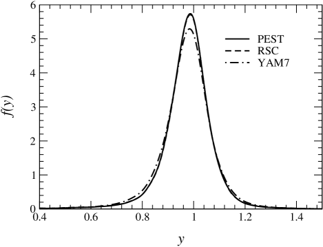
FIG. 1.: Neutron light cone momentum distribution in ³He for various potentials.

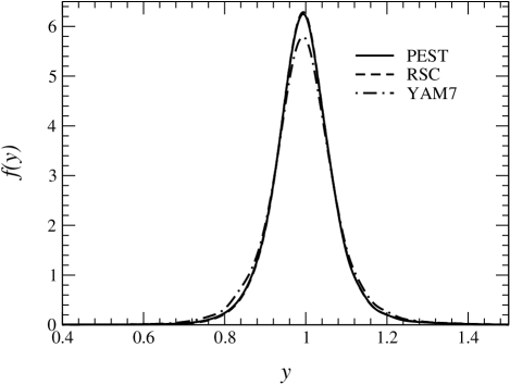
FIG. 2.: Proton light cone momentum distribution in ³He for various potentials.

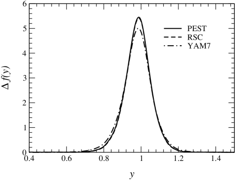
FIG. 3.: Neutron polarised light cone momentum distribution in ³He for various potentials.

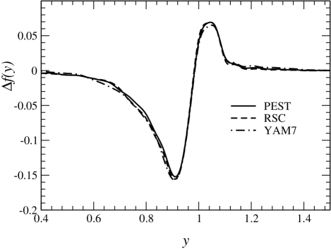
FIG. 4.: Proton polarised light cone momentum distribution in ³He for various potentials.

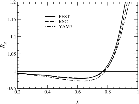
FIG. 5.: The ratio $R_{3}$, given in Eq.(76), for ³He, at $Q^{2}=10$GeV², calculated for various potentials using the CTEQ5 quark distributions.

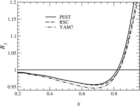
FIG. 6.: The ratio $R_{3}$, given in Eq.(76), for ³H, at $Q^{2}=10$GeV², calculated for various potentials using the CTEQ5 quark distributions.

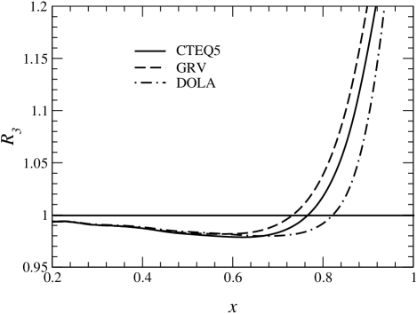
FIG. 7.: The ratio $R_{3}$, given in Eq.(76), for ³He, at $Q^{2}=10$GeV², calculated for the PEST potential, using various quark distributions for the nucleons.

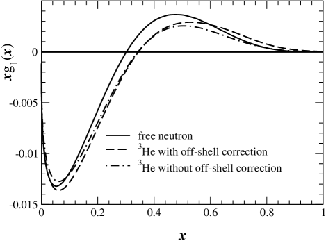
FIG. 8.: Comparison of several calculations of $xg_{1}(x)$ for ³He, at $Q^{2}=10GeV^{2}$.

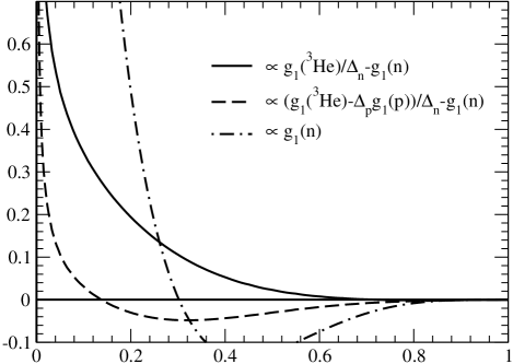
FIG. 9.: $\Delta_{g}$, $\Delta^{{}^{\prime}}_{g}$ and $g_{1}(n)$ at $Q^{2}=10GeV^{2}$. Note that all three curves have been divided by $\int dxg_{1}(^{3}He)$.

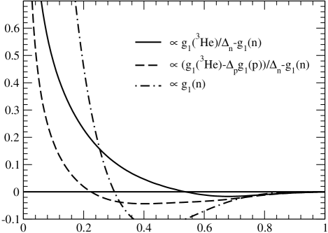
FIG. 10.: $\Delta_{g}$, $\Delta^{{}^{\prime}}_{g}$ and $g_{1}(n)$, including off-shell corrections, at $Q^{2}=10GeV^{2}$. Note that all three curves have been divided by $\int dxg_{1}(^{3}He)$.

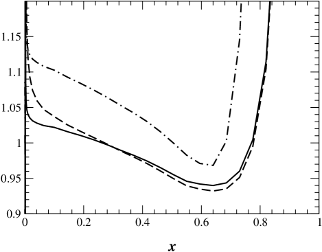
FIG. 11.: $R_{g}$ and $R^{{}^{\prime}}_{g}$ at $Q^{2}=10GeV^{2}$.

REFERENCES

- [1] J. Haidenbauer and W. Plessas Phys. Rev. C 30, 1822 (1984), C 32, 1424 (1985).
- [2] M. Lacombe, B. Loiseau, J. M. Richard, R. Vinh Mau, J. Côtè, P. Pirès, and R. de Tourreil Phys. Rev. C 21, 861 (1980).
- [3] W. C. Parke, Y. Koike, D. R. Lehman and L. C. Maximon Few Body Syst. 11, 89 (1991).
- [4] T. Y. Saito and I. R. Afnan Phys. Rev. C 50, 2756 (1994); Few Body Syst. 18, 101 (1995).
- [5] I. R. Afnan and J. M. Read, Aust. J. Phys. 26 725 (1973); Phys. Rev. C 8,1294 (1973).
- [6] R. V. Reid, Ann. Phys. (N.Y.) 50, 411 (1968).
- [7] Y. Yamaguchi and Y. Yamaguchi, Phys. Rev. 95, 1635 (1954).
- [8] I. R. Afnan and A. W. Thomas: “Fundamentals of Three-Body Scattering Theory” in Modern Three-Hadron Physics, ed. A. W. Thomas (Springer-Verlag, Berlin Heidelberg New York, 1977).
- [9] C. Lovelace, Phys. Rev. 135B, 1225 (1964).
- [10] I. R. Afnan and N. D. Birrell, Phys. Rev. C 16, 823 (1977).
- [11] R. Machleidt, F. Sammarruca and Y. Song, Structure,” Phys. Rev. C53, 1483 (1996) [nucl-th/9510023].
- [12] B. F. Gibson, Nucl. Phys. A543, 1e (1992); M. T. Peña, P. U. Sauer, A. Stalder and G. Gortemeyer Phys. Rev. C 48, 2208 (1993); S. A. Coon and M. T. Peña Phys. Rev. C 48, 2559 (1993); T. Y. Saito and J. Haidenbauer Eur. Phys. J A7,559 (2000).
- [13] D. F. Geesaman, K. Saito and A. W. Thomas, Ann. Rev. Nucl. Part. Sci. 45, 337 (1995).
- [14] B. Lampe and E. Reya Phys. Rept. 332, 1 (2000).
- [15] M. Anselmino, A. Efremov and E. Leader Phys. Rept. 261, 1 (1995).
- [16] R. -W. Schulze and P. U. Sauer Phys. Rev. C 48, 38 (1993).
- [17] R. -W. Schulze and P. U. Sauer Phys. Rev. C 56, 2293 (1997).
- [18] T. Uchiyama and K. Saito Phys. Rev. C 38, 2245 (1988).
- [19] L. L. Frankfurt and M. I. Strikman Phys. Lett. B64,433 (1976); Phys. Lett. B65,51 (1976); Phys. Lett. B76,333 (1978) ; Nucl. Phys. B148,107; Phys. Rept. 76, 215 (1981).
- [20] H-M. Jung and G. A. Miller Phys. Lett. B200,351 (1988).
- [21] C. Ciofi degli Atti and S. Liuti, Phys. Rev. C41, 1100 (1990).
- [22] C. Ciofi degli Atti, E. Pace and G. Salmè, Phys. Lett 141B, 14 (1984).
- [23] S. Frullani and J. Mougey Adv. in Nucl. Phys. 14, 1 (1984).
- [24] A. E. L. Dieperink and T. de Forest Jr., Ann. Rev. Nucl. Sc. 25, 1 (1975).
- [25] J. L. Friar, B. F. Gibson, G. L. Payne, A. M. Bernstein and T. E. Chupp, Phys. Rev. C42, 2310 (1990).
- [26] J. J. Aubert et al., Phys. Lett. 123B, 275 (1983).
- [27] H. L. Lai, J. Huston, S. Kuhlmann, J. Morfin, F. Olness, J. F. Owens, J. Pumplin, W. K. Tung HEP-ph/9903282.
- [28] M. Glück, E. Reya and A. Vogt, Z. Phys. C 67, 433 (1995).
- [29] A. Donnachie and P. V. Landshoff, Z. Phys. C 61, 139 (1994).
- [30] J. T. Londergan and A. W. Thomas, Prog. Part. Nucl. Phys. 41, 49 (1998).
- [31] R. M. Woloshyn Nucl. Phys. A496, 749 (1989); B. Blankleider and R. M. Woloshyn, Phys. Rev. C 29, 538 (1984).
- [32] Y. Goto et al. [Asymmetry Analysis collaboration], Phys. Rev. D 62, 034017 (2000) [hep-ph/0001046].
- [33] M. Glück, E. Reya, M. Stratmann and W. Vogelsang, Phys. Rev. D 53, 4775 (1996).
- [34] F. M. Steffens, K. Tsushima, A. W. Thomas and K. Saito, Phys. Lett. B447, 233 (1999).
- [35] P. A. M. Guichon, K. Saito, E. Rodionov and A. W. Thomas, Nucl. Phys. A601, 349 (1996) [nucl-th/9509034]; K. Saito and A. W. Thomas, Phys. Rev. C51, 2757 (1995) [nucl-th/9410031]; P. A. Guichon, Phys. Lett. B200, 235 (1988).
- [36] T. Gherman and W. J. Stirling Z. Phys. C 65, 461 (1995).
- [37] I. R. Afnan et al., Phys. Lett. B493, 36 (2000) [nucl-th/0006003].
- [38] G. G. Petratos et al., Jefferson Lab proposal (July 2000)
- [39] E. Pace, G. Salme and S. Scopetta, To appear in Nucl. Phys. A, nucl-th/0009028.
- [40] R. J. Ord-Smith, Phys. Rev. 94, 1227 (1954).