Exact spinor-scalar bound states in a QFT with scalar interactions

Abstract

We study two-particle systems in a model quantum field theory, in which scalar particles and spinor particles interact via a mediating scalar field. The Lagrangian of the model is reformulated by using covariant Green’s functions to solve for the mediating field in terms of the particle fields. This results in a Hamiltonian in which the mediating-field propagator appears directly in the interaction term. It is shown that exact two-particle eigenstates of the Hamiltonian can be determined. The resulting relativistic fermion-boson equation is shown to have Dirac and Klein-Gordon one-particle limits. Analytic solutions for the bound state energy spectrum are obtained for the case of massless mediating fields.

I Introduction

There are few examples of analytically solvable relativistic two-body wave equations, particularly equations derived from quantum field theory(QFT). The principal exception is the case of spinless (scalar) particles interacting via a mediating scalar field, the so-called scalar Yukawa or Wick-Cutkosky model. This model, therefore, has served as a favourite testing ground for methods of solving bound-state problems in QFT, beginning with the Wick [1] and Cutkosky [2] solution of the Bethe-Salpeter equation in ladder approximation.

In earlier papers [3, 4] it was shown that the scalar Yukawa model can be recast in a form such that exact two-body eigenstates of the Hamiltonian, in the canonic equal-time formalism, can be determined for the case where there are no free (physical) quanta of the mediating “chion” field (i.e. only virtual chions). This is achieved by the partial elimination of the mediating chion field by means of Green functions, by the use of the Feshbach-Villars formulation for the scalar particle fields, and by the use of an “empty” vacuum state. The resulting two-particle bound state mass spectrum, for the case of massless chion exchange, was found to be

$$E_{\pm}=\sqrt{m_{1}^{2}+m_{2}^{2}\pm 2m_{1}m_{2}\sqrt{1-{\alpha^{2}\over n^{2}}}},$$ (1.1)

where $\alpha$ is the effective dimensionless coupling constant, and $n=1,2,...$ is the principal quantum number.

The expression (1.1) for $E(\alpha/n)$ has the shape of a distorted semicircle. Indeed, in terms of the variables $x=(E^{2}-m_{1}^{2}-m_{2}^{2})/2m_{1}m_{2}$ and $y=\alpha/n$, (1.1) corresponds to half of the circle $x^{2}+y^{2}=1$. The upper branch $E_{+}$ of the energy eigenvalue (1.1) starts at $m_{1}+m_{2}$ when $\alpha$ is zero, and decreases monotonically to the value $E_{c}=\sqrt{m_{1}^{2}+m_{2}^{2}}$ when $\alpha$ reaches the critical value $\alpha_{c}=n$, beyond which the energy ceases to be real. This behaviour is reminiscent of what happens for the one-body Klein-Gordon-Coulomb and Dirac-Coulomb systems. From $\displaystyle E_{+}=m_{1}+m_{2}-{1\over 2}{{m_{1}m_{2}}\over{m_{1}+m_{2}}}{\alpha^{2}\over n^{2}}+O(\alpha^{4})$ it is clear that $E_{+}(\alpha)$ has the correct non-relativistic Schrödinger (Balmer) limit. It also has the expected Klein-Gordon one-body limit (with scalar Coulombic potential), namely $E_{\pm}-m_{1}\to\pm m_{2}\,\sqrt{1-\alpha^{2}/n^{2}}$ as $m_{1}\to\infty$.

The lower branch, $E_{-}$, which starts from $|m_{1}-m_{2}|$, rises monotonically with increasing $\alpha$ to meet the upper branch at $E_{c}$. From $\displaystyle~{}E_{-}=|m_{1}-m_{2}|+{1\over 2}\left({{m_{1}m_{2}}\over{|m_{1}-m_{2}|}}\right){\alpha^{2}\over n^{2}}+O(\alpha^{4})~{}$ for $m_{1}\neq m_{2}$, and $\displaystyle~{}E_{-}=m\frac{\alpha}{n}+O(\alpha^{3})~{}$ for $m_{1}=m_{2}=m$, it is clear that the lower branch does not have the Balmer limit at small $\alpha$, and so is ‘unphysical’ in this sense. The ‘unphysical’ lower branch arises because an ‘empty’ vacuum was used, so that positive and negative energy solutions (rather than particles and antiparticles) are retained, and this means that solutions with two-body energies of the type $m_{1}+m_{2},m_{1}-m_{2},-m_{1}+m_{2},-m_{1}-m_{2}$ occur. However, the use of the empty vacuum is the price that needs to be paid for obtaining analytic solutions.

Interestingly, the same spectrum (1.1) was obtained previously by Berezin, Itzykson and Zinn-Justin [5] as poles of the scattering matrix in eikonal approximation, by Todorov [6], using a “quasipotential” one-time reduction of the ladder Bethe-Salpeter equation, by Savrin and Troole [7] as a solution of the ladder Bethe-Salpeter equation with retarding propagators, and recently by Tretyak and Shpytko [8] in a Fokker action formulation. Berezin, Itzykson and Zinn-Justin state that their analysis implies that (1.1) contains, in perturbation-theory language, all recoil, ladder and crossed ladder effects, but no radiative corrections. However, as has been pointed out recently [9], the results analogous to (1.1) but for the massive chion exchange case (specifically for $\mu/m=0.15$), lie somewhat above the numerical Feynman-Schwinger calculations of Nieuwenhuis and Tjon [10], which contain all effects save for radiative corrections.

The method of elimination of mediating fields, used in [3, 4], is to some extend similar to that used in the formalism of Fokker action integrals in relativistic mechanics. Although the Fokker action formalism deals with a finite number of degrees of freedom, in the case of scalar interactions its quantized counterpart [8] leads to the same expression (1.1) for the energy as a function of quantum number $n$ as that obtained in [3, 4]. The difference is in different definitions of $n$ in the two treatments. This is due to different definitions of scalar interactions in the mechanical and QFT pictures, and by quantization ambiguities of the classical Fokker action.

It is evidently of interest to extend the method employed in [3, 4] to include spinor particle fields. As a first step we consider a generalized Yukawa model consisting of fermions, described by a spinor field $\Psi$, and of bosons, described by a scalar field $\varphi$, interacting via a mediating scalar field $\chi$. Our starting point is the Lagrangian density ($c=\hbar=1$)

$${\cal L}=\bar{\Psi}(i\gamma^{\nu}\partial_{\nu}-g_{1}\chi-m_{1})\Psi+\partial_{\nu}\varphi^{*}\partial^{\nu}\varphi-m_{2}^{2}\varphi^{*}\varphi-g_{2}\varphi^{*}\varphi\chi+\frac{1}{2}\partial_{\nu}\chi\partial^{\nu}\chi-\frac{1}{2}\mu^{2}\chi^{2}$$ (1.2)

The fields of the model (1.2) satisfy the equations

$$(i\gamma^{\nu}\partial_{\nu}-g_{1}\chi-m_{1})\Psi =0,$$ (1.3)

$$(\partial_{\nu}\partial^{\nu}+m_{2}^{2}+g_{2}\chi)\varphi =0,$$ (1.4)

and the conjugates of (1.3) and (1.4), as well as

$$(\partial_{\nu}\partial^{\nu}+\mu^{2})\chi=\rho,$$ (1.5)

with

$$\rho=-(g_{1}\bar{\Psi}\Psi+g_{2}\varphi^{*}\varphi)$$ (1.6)

Equation (1.5) has the formal solution

$$\chi=\chi_{0}+\chi_{1},$$ (1.7)

where

$$\chi_{1}={\langle}D*\rho{\rangle}:=\int dx^{\prime}D(x-x^{\prime})\rho(x^{\prime}),$$ (1.8)

$dx=d^{N}x\,dt$ (in $N+1$ dimensions), and $\chi_{0}(x)$ satisfies the homogeneous (or free field) equation,

$$(\partial_{\nu}\partial^{\nu}+\mu^{2})\chi_{0}=0,$$ (1.9)

while $D(x-x^{\prime})$ is a covariant Green function (or chion propagator, in the language of QFT), such that

$$(\partial_{\nu}\partial^{\nu}+\mu^{2})D(x-x^{\prime})=\delta^{N+1}(x-x^{\prime}).$$ (1.10)

Equation (1.10) does not specify $D(x-x^{\prime})$ uniquely since, for example, any solution of the homogeneous equation can be added to it without invalidating (1.10). This allows for a certain freedom in the choice of $D(x)$, as is discussed in standard texts (e.g. refs. [11, 12]). Substitution of the formal solution (1.7) into Eqs. (1.3) and (1.4) yields the “reduced” equations

$$\left(i\gamma^{\nu}\partial_{\nu}-g_{1}(\chi_{0}+\chi_{1})-m_{1}\right)\Psi=0,$$ (1.11)

$$(\partial_{\nu}\partial^{\nu}+m_{2}^{2})\varphi=-g_{2}(\chi_{0}+\chi_{1})\varphi.$$ (1.12)

These equations are derivable from the action principle $\displaystyle\delta\int dx\,{\cal L}=0$, corresponding to the Lagrangian density

$${\cal L}=\bar{\Psi}(i\gamma^{\nu}\partial_{\nu}-m_{1})\Psi+\partial_{\nu}\varphi^{*}\partial^{\nu}\varphi-m_{2}^{2}\varphi^{*}\varphi+\chi_{0}\rho+\frac{1}{2}\rho{\langle}D*\rho{\rangle}$$ (1.13)

provided that $D(x-x^{\prime})=D(x^{\prime}-x)$.

The QFTs based on (1.2) and (1.13) are equivalent in the sense that they lead to identical invariant matrix elements in various order of covariant perturbation theory. The difference is that, in the formulation based on (1.13), the interaction term that contains the chion propagator $D(x-x^{\prime})$ leads to Feynman diagrams that correspond to processes involving virtual chions only. On the other hand, the interaction term that contains $\chi_{0}$ corresponds to Feynman diagrams that cannot be generated by the previous term, such as those with external (physical) chion lines.

The reformulated Lagrangian (1.13) contains two types of interactions: “local” interactions, $\chi_{0}\rho$, of the particle densities $\varphi^{*}(x)\varphi(x)$ and $\bar{\Psi}(x)\Psi(x)$ with the free mediating field $\chi_{0}(x)$, and the “nonlocal” interaction, $\frac{1}{2}\rho{\langle}D*\rho{\rangle}$, in which the chion propagator appears explicitly. This may seem like a complication rather than simplification of the theory based on (1.2). However, as we will show, the form (1.13) leads to a model for which exact eigenstates of the Hamiltonian can be obtained.

II Feshbach-Villars Formulation of the Scalar Field

We rewrite the scalar field $\varphi$ of this model in the Feshbach-Villars (FV) formulation [13]. The reason for doing so is that this leads to a QFT Hamiltonian which is Schrödinger-like in form, for which exact eigensolutions can be obtained. In the FV formulation, the field $\varphi$ and its time-derivative $\dot{\varphi}$ are replaced by a two-component vector which is defined as

$$\phi=\left[\matrix{\phi_{1}={1\over{\sqrt{2m_{2}}}}(m_{2}\varphi+i\dot{\varphi})&\cr\phi_{2}={1\over{\sqrt{2m_{2}}}}(m_{2}\varphi-i\dot{\varphi})&\cr}\right]\;\;\;$$ (2.1)

so that, for example, $2m_{2}\,\varphi^{*}\varphi=(\phi_{1}^{*}+\phi_{2}^{*})(\phi_{1}+\phi_{2})=\phi^{{\dagger}}\eta\tau\phi$, where $\eta$ and $\tau$ are the matrices

$$\eta=\left[\matrix{1&0\cr 0&-1\cr}\right]\;\;\;\;{\rm and}\;\;\;\;\tau=\left[\matrix{1&1\cr-1&-1\cr}\right].$$ (2.2)

In the FV formulation the equation of motion (1.4) takes on the form

$$i\dot{\phi}=-{1\over{2m_{2}}}\nabla^{2}\tau\phi+m_{2}\eta\phi+{g_{2}\over{2m_{2}}}\tau\phi\chi,$$ (2.3)

or, upon using (1.7), the form

$$i\dot{\phi}=-{1\over{2m_{2}}}\nabla^{2}\tau\phi+m_{2}\eta\phi+{g_{2}\over{2m_{2}}}\tau\phi(\chi_{0}+{\langle}D*\rho{\rangle}),$$ (2.4)

where $\displaystyle\rho=-(g_{1}\bar{\Psi}\Psi+{g_{2}\over{2m_{2}}}{\phi^{\dagger}}\eta\tau\phi)$.

Equations (2.4) and (1.11) are derivable from the Lagrangian density

$${\cal L}_{FV}=\bar{\Psi}(i\gamma^{\nu}\partial_{\nu}-m_{1})\Psi+i\phi^{{\dagger}}(x)\eta\dot{\phi}(x)-{1\over{2m_{2}}}\nabla{\overline{\phi}}(x)\cdot\nabla\phi(x)-m_{2}\phi^{{\dagger}}(x)\phi(x)+\chi_{0}\rho+\frac{1}{2}\rho{\langle}D*\rho{\rangle},$$ (2.5)

where ${\overline{\phi}}=\phi^{{\dagger}}\eta\tau\phi$.

III Quantization

The momenta corresponding to $\phi_{1}$ and $\phi_{2}$ are

$$p_{\phi_{1}}={{\partial}{\cal L}_{FV}\over{{\partial}\dot{\phi_{1}}}}=i\phi_{1}^{*},~{}~{}~{}~{}p_{\phi_{2}}=-i\phi_{2}^{*}$$ (3.1)

Thus, the Hamiltonian density is given by the expression

$${\cal H}(x)=\Psi^{\dagger}(x){\hat{h}_{1}}(x)\Psi(x)+\phi^{{\dagger}}(x)\eta{\hat{h}_{2}}(x)\phi(x)-\chi_{0}(x)\rho(x)-\frac{1}{2}\rho(x){\langle}D*\rho{\rangle}$$ (3.2)

where $\displaystyle{\hat{h}_{1}}(x)=-i\vec{\alpha}\cdot\nabla+m_{1}\beta,~{}{\hat{h}_{2}}(x)=\tau\left(-{1\over{2m_{2}}}\right)\nabla^{2}+m_{2}\,\eta$, and where we have suppressed terms like $\nabla\cdot({\overline{\phi}}(x)\nabla\phi(x))$ that vanish upon integration and application of Gauss’ theorem. We use canonical equal-time quantization, whereupon the non-vanishing anticommutation relations, and commutation relations, are

$$\{\Psi_{\alpha}(\mbox{\boldmath$x$},t),\Psi_{\beta}(\mbox{\boldmath$y$},t)^{\dagger}\}=\delta_{\alpha\beta}\delta^{N}(\mbox{\boldmath$x$}-\mbox{\boldmath$y$}),~{}~{}~{}\alpha,\beta=1...4;~{}~{}~{}[\phi_{a}(\mbox{\boldmath$x$},t),\phi^{{\dagger}}_{b}(\mbox{\boldmath$y$},t)]=\eta_{ab}\delta^{N}(\mbox{\boldmath$x$}-\mbox{\boldmath$y$}),\;\;\;a,b=1,2$$ (3.3)

where $\eta_{ab}$ are elements of the $\eta$ matrix (2.2). Using these commutation relations, the Hamiltonian operator can be written as

$$H=\int d^{N}x\,[{\cal H}_{0}(x)+{\cal H}_{\chi}(x)+{\cal H}_{I}(x)],$$ (3.4)

where (suppressing the Hamiltonian of the free chion field),

$${\cal H}_{0}(x) = \Psi^{\dagger}(x){\hat{h}_{1}}(x)\Psi(x)+\phi^{{\dagger}}(x)\eta{\hat{h}_{2}}(x)\phi(x),$$ (3.5)

$${\cal H}_{\chi}(x) = -\chi_{0}(x)\rho(x)$$ (3.6)

and

$$;{\cal H}_{I}(x);\;\;\;= - {g_{1}^{2}\over{2}}\int dx^{\prime}\,D(x-x^{\prime})\,{\overline{\Psi}}(x)({\overline{\Psi}}(x^{\prime})\Psi(x^{\prime}))\Psi(x){}$$ (3.7)

$$- {g_{2}^{2}\over{8m_{2}^{2}}}\int dx^{\prime}\,D(x-x^{\prime})\,{\overline{\phi}}(x)({\overline{\phi}}(x^{\prime})\phi(x^{\prime}))\phi(x){}$$ (3.8)

$$- {{g_{1}g_{2}}\over{4m_{2}}}\int dx^{\prime}\,D(x-x^{\prime})\,{\overline{\phi}}(x)({\overline{\Psi}}(x^{\prime})\Psi(x^{\prime}))\phi(x){}$$ (3.9)

$$- {{g_{1}g_{2}}\over{4m_{2}}}\int dx^{\prime}\,D(x-x^{\prime})\,{\overline{\Psi}}(x)({\overline{\phi}}(x^{\prime})\phi(x^{\prime}))\Psi(x),$$ (3.10)

and where we have used the commutation relations (3.3) to reorder ${\overline{\phi}}(x)\phi(x){\overline{\phi}}(x^{\prime})\phi(x^{\prime})$ as ${\overline{\phi}}(x)({\overline{\phi}}(x^{\prime})\phi(x^{\prime}))\phi(x)$ and ${\overline{\Psi}}(x)\Psi(x){\overline{\Psi}}(x^{\prime})\Psi(x^{\prime})$ as ${\overline{\Psi}}(x)({\overline{\Psi}}(x^{\prime})\Psi(x^{\prime}))\Psi(x)$. Note that no infinities are dropped upon performing the ‘normal ordering’ of scalar field operators, since none arise on account of the property that $\tau^{2}=0$. However, in the case of the spinor field, reordering yields an infinite constant which can be absorbed into the total energy of the system. Of course, one can simply start from the normal-ordered Hamiltonian. We stress that this ‘normal ordering’ is not the same as the conventional one [14], since we normal order the entire field operators, $\phi,\psi$ and $\phi^{{\dagger}},\psi^{{\dagger}}$, not positive and negative frequency parts individually. For this reason, we denote it as $;H;$ rather than as $:H:$.

As already mentioned, ${\cal H}_{I}$ contains the covariant chion propagator, hence in conventional covariant perturbation theory it leads to Feynman diagrams with internal chion lines. On the other hand, ${\cal H}_{\chi}$ leads to Feynman diagrams with external chions. However, we shall not pursue covariant perturbation theory in this work, and so shall not consider that approach further. Rather, we shall consider an approach that leads to some exact eigenstates of the Hamiltonian (3.4), but with ${\cal H}_{\chi}=0$.

IV Truncated model

In what follows we shall consider the truncated model for which the term ${\cal H}_{\chi}$ in (3.4) is suppressed. Such a Hamiltonian is appropriate for describing systems for which there is no annihilation or decay into chions, or chion-phion/psion scattering.

In the Schrödinger picture we can take $t=0$. Therefore, we shall use the notation that, say $\phi(\mbox{\boldmath$x$},t=0)=\phi(\mbox{\boldmath$x$})$, etc., for the QFT operators. This allows us to express the interaction part of the Hamiltonian (3.7) as

$$;{\cal H}_{I}(x);\;\;\;= - {g_{1}^{2}\over{2}}\int d^{N}x^{\prime}\,G(\mbox{\boldmath$x$}-\mbox{\boldmath$x^{\prime}$})\,{\overline{\Psi}}(\mbox{\boldmath$x$})({\overline{\Psi}}(\mbox{\boldmath$x^{\prime}$})\Psi(\mbox{\boldmath$x^{\prime}$}))\Psi(\mbox{\boldmath$x$}){}$$ (4.1)

$$- {g_{2}^{2}\over{8m_{2}^{2}}}\int d^{N}x^{\prime}\,G(\mbox{\boldmath$x$}-\mbox{\boldmath$x^{\prime}$})\,{\overline{\phi}}(\mbox{\boldmath$x$})({\overline{\phi}}(\mbox{\boldmath$x^{\prime}$})\phi(\mbox{\boldmath$x^{\prime}$}))\phi(\mbox{\boldmath$x$}){}$$ (4.2)

$$- {{g_{1}g_{2}}\over{4m_{2}}}\int d^{N}x^{\prime}\,G(\mbox{\boldmath$x$}-\mbox{\boldmath$x^{\prime}$})\,{\overline{\phi}}(\mbox{\boldmath$x$})({\overline{\Psi}}(\mbox{\boldmath$x^{\prime}$})\Psi(\mbox{\boldmath$x^{\prime}$}))\phi(\mbox{\boldmath$x$}){}$$ (4.3)

$$- {{g_{1}g_{2}}\over{4m_{2}}}\int d^{N}x^{\prime}\,G(\mbox{\boldmath$x$}-\mbox{\boldmath$x^{\prime}$})\,{\overline{\Psi}}(\mbox{\boldmath$x$})({\overline{\phi}}(\mbox{\boldmath$x^{\prime}$})\phi(\mbox{\boldmath$x^{\prime}$}))\Psi(\mbox{\boldmath$x$}),$$ (4.4)

where

$$G(\mbox{\boldmath$x$}-\mbox{\boldmath$x^{\prime}$})=\int_{-\infty}^{\infty}D(x-x^{\prime})\,dt^{\prime}={1\over{(2\pi)^{N}}}\int d^{N}p\,e^{i\mbox{\boldmath$p$}\cdot(\mbox{\boldmath$x$}-\mbox{\boldmath$x^{\prime}$})}{1\over{\mbox{\boldmath$p$}^{2}+\mu^{2}}}\,.$$ (4.5)

Explicitly, for $N=3$ spatial dimensions this becomes

$$G(\mbox{\boldmath$x$}-\mbox{\boldmath$x^{\prime}$})={1\over{4\pi}}{e^{-\mu|\mbox{\boldmath$x$}-\mbox{\boldmath$x^{\prime}$}|}\over{|\mbox{\boldmath$x$}-\mbox{\boldmath$x^{\prime}$}|}},$$ (4.6)

for $N=2$ it is

$$G(\mbox{\boldmath$x$}-\mbox{\boldmath$x^{\prime}$})={1\over{2\pi}}k_{0}(\mu|\mbox{\boldmath$x$}-\mbox{\boldmath$x^{\prime}$}|),$$ (4.7)

where $k_{0}(z)$ is the modified Bessel function, whereas for $N=1$ it has the form

$$G(x-x^{\prime})={1\over{2\mu}}e^{-\mu|x-x^{\prime}|}$$ (4.8)

V Empty vacuum and one-particle eigenstates

As in Refs. [3, 4], we define an empty vacuum state, $|\tilde{0}\rangle$, such that

$$\phi_{a}|\tilde{0}\rangle=\Psi_{\alpha}|\tilde{0}\rangle=0.$$ (5.1)

This is different from the “Dirac vacuum” $|0\rangle$ of conventional QFT, which is annihilated by only the positive frequency part of $\varphi$ and $\Psi$ and by the negative frequency parts of $\varphi^{{\dagger}}$ and $\Psi^{{\dagger}}$.

With the definition (5.1), the one-particle scalar state defined as

$$|1_{\phi}\rangle=\int d^{N}x\,{\phi^{\dagger}}(\mbox{\boldmath$x$})\eta f(\mbox{\boldmath$x$})|\tilde{0}\rangle,$$ (5.2)

where $f(\mbox{\boldmath$x$})$ is a two-component vector, is an eigenstate of the truncated QFT Hamiltonian (${\cal H}_{\chi}=0$) with eigenvalue $E_{1}$ provided that the $f(\mbox{\boldmath$x$})$ is a solution of the equation

$${\hat{h}_{2}}(\mbox{\boldmath$x$})f(\mbox{\boldmath$x$})=E_{1}f(\mbox{\boldmath$x$}).$$ (5.3)

This is just the free-particle Klein-Gordon equation for stationary states (in Feshbach-Villars form). It has, of course, all the usual negative-energy “pathologies” of the KG equation. The presence of negative-energy solutions is a consequence of the use of the empty vacuum.

Similarly, the state

$$|1_{\Psi}{\rangle}=\int d^{3}x\,\tilde{F}_{\alpha}(\mbox{\boldmath$x$})\,\Psi^{{\dagger}}_{\alpha}(x)|{\widetilde{0}}{\rangle},$$ (5.4)

is an eigenstate of $;H;$ with eigenenergy $E_{1}$, provided that the four coefficient amplitudes $\tilde{F}_{\alpha}(\mbox{\boldmath$x$})$ are solutions of

$$\{[h_{1}(\mbox{\boldmath$x$})]_{\alpha\,\beta}-{E}_{1}\,\delta_{\alpha\,\beta}\}\tilde{F}_{\beta}(\mbox{\boldmath$x$})=0,$$ (5.5)

or

$$(h_{1}(\mbox{\boldmath$x$})-E_{1})\tilde{F}(\mbox{\boldmath$x$})=0$$ (5.6)

in matrix notation, that is provided the spinor $\tilde{F}$ is a solution of the usual Dirac eigenvalue equation (5.6). Note that summation on repeated spinor indices $\alpha,\beta$ is implied in equations (5.4) and (5.5).

VI Two-particle eigenstates

We consider a mixed two-particle phion-plus-psion system described by

$$|2\rangle=\int d^{N}x\,d^{N}y\;F_{\alpha\,j}(\mbox{\boldmath$x$},\mbox{\boldmath$y$})\;{\Psi^{\dagger}}_{\alpha}(\mbox{\boldmath$x$}){\phi^{\dagger}}_{j}(\mbox{\boldmath$y$})|\tilde{0}\rangle$$ (6.1)

where summation on repeated spinor and boson indices, $\alpha$ and $j$, is implied. This state is an exact eigenstate of the truncated QFT Hamiltonian ((3.4) with ${\cal H}_{\chi}=0$) provided that the $4\times 2$ coefficient matrix $F=[F_{\alpha\,j}]$ is a solution of the two-body equation,

$${\hat{h}_{1}}(\mbox{\boldmath$x$})F+\left[\eta{\hat{h}_{2}}(\mbox{\boldmath$y$})\eta F^{\rm T}(\mbox{\boldmath$x$},\mbox{\boldmath$y$})\right]^{\rm T}+V(\mbox{\boldmath$x$}-\mbox{\boldmath$y$})\gamma^{0}\left[\eta\tau\eta F^{\rm T}(\mbox{\boldmath$x$},\mbox{\boldmath$y$})\right]^{\rm T}=EF$$ (6.2)

where the superscript T stands for “transpose”. The potential here is given by

$$V(\mbox{\boldmath$x$}-\mbox{\boldmath$y$})=-\frac{g_{1}g_{2}}{2m_{2}}G(\mbox{\boldmath$x$}-\mbox{\boldmath$y$})$$ (6.3)

where $G(\mbox{\boldmath$x$}-\mbox{\boldmath$y$})$ is specified in equations (4.5)-(4.8). Alternatively, we can regard $|2{\rangle}$ as a variational approximation to the eigenstate of the complete Hamiltonian (3.4), since ${\langle}2|H_{\chi}|2{\rangle}=0$.

For $|2{\rangle}$ to be an eigenstate of the momentum operator with eigenvalue $\mbox{\boldmath$P$}_{TOTAL}=0$, it is necessary that the 4$\times$2 ‘hyperspinor’ $F(\mbox{\boldmath$x$},\mbox{\boldmath$y$})$ be of the form $F(\mbox{\boldmath$r$})$, where $\mbox{\boldmath$r$}=\mbox{\boldmath$x$}-\mbox{\boldmath$y$}$. Let us define

$$F(\mbox{\boldmath$r$})=\left[\matrix{s(\mbox{\boldmath$r$})\cr t(\mbox{\boldmath$r$})}\right],$$ (6.4)

where, in $N=3$ spatial dimensions,

$$s(\mbox{\boldmath$r$})=\left[\matrix{F_{11}(\mbox{\boldmath$r$})&F_{12}(\mbox{\boldmath$r$})\cr F_{21}(\mbox{\boldmath$r$})&F_{22}(\mbox{\boldmath$r$})\cr}\right],~{}~{}~{}~{}t(\mbox{\boldmath$r$})=\left[\matrix{F_{31}(\mbox{\boldmath$r$})&F_{32}(\mbox{\boldmath$r$})\cr F_{41}(\mbox{\boldmath$r$})&F_{42}(\mbox{\boldmath$r$})\cr}\right].$$ (6.5)

Then equation (6.2) can be written as two coupled equations for the 2$\times$2-matrices $s(\mbox{\boldmath$r$}),~{}t(\mbox{\boldmath$r$})$

$$-i\mbox{\boldmath$\sigma$}\cdot\mbox{\boldmath$\bigtriangledown$}t(\mbox{\boldmath$r$})+\left[\eta\Big{(}\hat{h}_{2}(\mbox{\boldmath$r$})+\tau V(\mbox{\boldmath$r$})\Big{)}\eta\,s^{\rm T}(\mbox{\boldmath$r$})\right]^{\rm T}+(m_{1}-E)s(\mbox{\boldmath$r$})=0,$$ (6.6)

$$-i\mbox{\boldmath$\sigma$}\cdot\mbox{\boldmath$\bigtriangledown$}s(\mbox{\boldmath$r$})+\left[\eta\Big{(}\hat{h}_{2}(\mbox{\boldmath$r$})-\tau V(\mbox{\boldmath$r$})\Big{)}\eta\,t^{\rm T}(\mbox{\boldmath$r$})\right]^{\rm T}-(m_{1}+E)t(\mbox{\boldmath$r$})=0.$$ (6.7)

In the absence of interactions (i.e. $V=0$), these equations have solutions with the following four types of energy eigenvalues: $\omega(\mbox{\boldmath$p$},m_{1})+\omega(\mbox{\boldmath$p$},m_{2})$, $-\omega(\mbox{\boldmath$p$},m_{1})+\omega(\mbox{\boldmath$p$},m_{2})$, $\omega(\mbox{\boldmath$p$},m_{1})-\omega(\mbox{\boldmath$p$},m_{2})$, $-\omega(\mbox{\boldmath$p$},m_{1})-\omega(\mbox{\boldmath$p$},m_{2})$, where $\omega(\mbox{\boldmath$p$},m)=\sqrt{\mbox{\boldmath$p$}^{2}+m^{2}}$. The first and last are positive and negative energy eigenvalues, respectively, while the middle two are ‘mixed’. The appearance of the negative energies is a reflection of our use of the empty vacuum state, as discussed earlier.

VII $J^{P}$ eigenstates and radial reduction in $N=3$ dimensions

The Hamiltonian (3.4) of the theory commutes with the total angular momentum and parity operators. If the two-particle state (6.1) is to be an eigenstate of $J_{3}$ where

$$\mbox{\boldmath$J$}=\int d^{3}x\,\Psi^{{{\dagger}}}(\mbox{\boldmath$x$},t)\,{\mbox{\boldmath$j$}}(\mbox{\boldmath$x$})\,\Psi(\mbox{\boldmath$x$},t)+\int d^{3}x\,\phi^{{\dagger}}(\mbox{\boldmath$x$},t)\eta\,\mbox{\boldmath$l$}(\mbox{\boldmath$x$})\,\phi(\mbox{\boldmath$x$},t),$$ (7.1)

with $\mbox{\boldmath$j$}(\mbox{\boldmath$x$})=\mbox{\boldmath$l$}(\mbox{\boldmath$x$})+\mbox{\boldmath$s$}=-i\mbox{\boldmath$x$}\times\mbox{\boldmath$\bigtriangledown$}_{\mbox{\boldmath$x$}}+\frac{1}{2}\mbox{\boldmath$\sigma$}$, then we require that the hyperspinor $F$ (cf. Equation (6.1)) must satisfy the equation

$$(j_{3}(\mbox{\boldmath$x$})+l_{3}(\mbox{\boldmath$y$}))F(\mbox{\boldmath$x$},\mbox{\boldmath$y$})=m_{J}F(\mbox{\boldmath$x$},\mbox{\boldmath$y$})$$ (7.2)

In other words, in the rest frame where $\mbox{\boldmath$P$}_{TOTAL}|2{\rangle}=0\;|2{\rangle}$, we require that

$$\left(l_{3}(\mbox{\boldmath$r$})+{1\over 2}\sigma_{3}\right)F(\mbox{\boldmath$r$})=m_{j}F(\mbox{\boldmath$r$}).$$ (7.3)

In a similar fashion $\mbox{\boldmath$J$}^{2}|2{\rangle}=j(j+1)|2{\rangle}$ implies that the matrix $F$ in the rest frame must satisfy the equation

$$\left(\mbox{\boldmath$l$}^{2}+{3\over 4}+\mbox{\boldmath$l$}\cdot\mbox{\boldmath$\sigma$}\right)F(\mbox{\boldmath$r$})=j(j+1)F(\mbox{\boldmath$r$})$$ (7.4)

The components $s,~{}t$ of $F$ satisfy Eqs. (7.3), (7.4) individually.

For $|2{\rangle}$ to be a parity eigenstate, and since $V(r)$ is invariant under space reflection the matrix $F(\mbox{\boldmath$r$})$ must have the property that

$$\beta F(\mbox{\boldmath$r$})=\pm F(-\mbox{\boldmath$r$}),$$ (7.5)

where the $\pm$ are the parity quantum numbers. This means that

$$s(-\mbox{\boldmath$r$})=\pm s(\mbox{\boldmath$r$}),~{}~{}~{}~{}t(-\mbox{\boldmath$r$})=\mp t(\mbox{\boldmath$r$}).$$ (7.6)

From Eqs. (7.3) - (7.6) it follows that

$$F(\mbox{\boldmath$r$})=\left[\matrix{s(\mbox{\boldmath$r$})\cr t(\mbox{\boldmath$r$})}\right]=\left[\matrix{k_{1}(r)\zeta_{j,m_{j}}^{\ell=j\pm\frac{1}{2}}(\hat{\mbox{\boldmath$r$}})&-k_{2}(r)\zeta_{j,m_{j}}^{\ell=j\pm\frac{1}{2}}(\hat{\mbox{\boldmath$r$}})\cr q_{1}(r)\zeta_{j,m_{j}}^{\lambda=j\mp\frac{1}{2}}(\hat{\mbox{\boldmath$r$}})&-q_{2}(r)\zeta_{j,m_{j}}^{\lambda=j\mp\frac{1}{2}}(\hat{\mbox{\boldmath$r$}})\cr}\right],~{}~{}~{}~{}\hat{\mbox{\boldmath$r$}}=\frac{\mbox{\boldmath$r$}}{r},$$ (7.7)

where the upper sign corresponds to parity ‘+’, and the lower to parity ‘-’, and $k_{1},~{}k_{2},~{}q_{1},~{}q_{2}$ are radial functions. The normalized “spinor harmonics” $\zeta_{j,m_{j}}^{\ell=j\pm\frac{1}{2}}(\hat{\mbox{\boldmath$r$}})$ are, explicitly,

$$\zeta_{j,m_{j}}^{\ell=j-\frac{1}{2}}(\hat{\mbox{\boldmath$r$}})=\frac{1}{\sqrt{2\ell+1}}\left[\matrix{\sqrt{\ell+m_{j}+\frac{1}{2}}Y_{\ell}^{m_{j}-\frac{1}{2}}(\hat{\mbox{\boldmath$r$}})\cr\sqrt{\ell-m_{j}+\frac{1}{2}}Y_{\ell}^{m_{j}+\frac{1}{2}}(\hat{\mbox{\boldmath$r$}})\cr}\right],$$ (7.8)

and

$$\zeta_{j,m_{j}}^{\ell=j+\frac{1}{2}}(\hat{\mbox{\boldmath$r$}})=\frac{1}{\sqrt{2\ell+1}}\left[\matrix{\sqrt{\ell-m_{j}+\frac{1}{2}}Y_{\ell}^{m_{j}-\frac{1}{2}}(\hat{\mbox{\boldmath$r$}})\cr-\sqrt{\ell+m_{j}+\frac{1}{2}}Y_{\ell}^{m_{j}+\frac{1}{2}}(\hat{\mbox{\boldmath$r$}})\cr}\right],$$ (7.9)

Finally, substituting (7.7) into (6.6), (6.7) we find that the radial functions must satisfy the following system of four equations:

$$\hat{\Pi}_{\sigma}^{\mp}q_{1}+\frac{\hat{\Pi}_{\pm}^{2}}{2m_{2}}(k_{1}+k_{2})+(m_{1}+m_{2})k_{1}+V(r)(k_{1}+k_{2})=Ek_{1},{}$$ (7.10)

$$\hat{\Pi}_{\sigma}^{\mp}q_{2}-\frac{\hat{\Pi}_{\pm}^{2}}{2m_{2}}(k_{1}+k_{2})+(m_{1}-m_{2})k_{2}-V(r)(k_{1}+k_{2})=Ek_{2},{}$$ (7.11)

$$\hat{\Pi}_{\sigma}^{\pm}k_{1}+\frac{\hat{\Pi}_{\mp}^{2}}{2m_{2}}(q_{1}+q_{2})+(-m_{1}+m_{2})q_{1}-V(r)(q_{1}+q_{2})=Eq_{1},$$ (7.12)

$$\hat{\Pi}_{\sigma}^{\pm}k_{2}-\frac{\hat{\Pi}_{\mp}^{2}}{2m_{2}}(q_{1}+q_{2})-(m_{1}+m_{2})q_{2}+V(r)(q_{1}+q_{2})=Eq_{2},{}$$ (7.13)

where $\displaystyle V(r)=-\alpha\frac{e^{-\mu r}}{r}$ with $\displaystyle\alpha=\frac{g_{1}g_{2}}{8\pi m_{2}}$, and where we have introduced the operators

$$\hat{\Pi}_{\sigma}^{\pm}:=-\frac{i}{r}\left(r\frac{d}{dr}+[1\pm(j+\frac{1}{2})]\right){}$$ (7.14)

(7.15)

$$\hat{\Pi}_{\pm}^{2}:=-\frac{1}{r}\left(r\frac{d^{2}}{dr^{2}}+2\frac{d}{dr}-\frac{(j+1/2)(j+1/2\pm 1)}{r}\right).{}$$ (7.16)

If we let $E=\varepsilon+m_{1}$ and consider the $m_{1}\to\infty$ limit of (7.10), we find that $q_{1},q_{2}\to 0$ while $k_{1}+k_{2}$ satisfies the radial Klein-Gordon equation (with scalar coupling). Similarly, if $m_{1}$ is replaced by $m_{2}$ in this procedure, then $k_{2},q_{2}\to 0$ while $q_{1}$ and $-ik_{1}$ satisfy the radial Dirac equations (with scalar coupling). Thus, equations (7.10) have the expected one-body limits.

Defining $q_{\pm}=q_{1}\pm q_{2},$ and $k_{\pm}=k_{1}\pm k_{2}$, then adding the first two, and separately the last two, of equations (7.10), we obtain

$$-i\frac{dq_{+}}{dr}=(E-m_{1})k_{+}-m_{2}k_{-}+\frac{i}{r}[1\mp(j+\frac{1}{2})]q_{+}{}$$ (7.17)

(7.18)

$$-i\frac{dk_{+}}{dr}=(E+m_{1})q_{+}-m_{2}q_{-}+\frac{i}{r}[1\pm(j+\frac{1}{2})]k_{+}{}$$ (7.19)

Using definitions (7.14), differentiating (7.17), and substituting the result into (7.10) we obtain

$${-}\frac{i}{2m_{2}}\left[(E+m_{1}+m_{2})q_{+}^{\prime}+\frac{m_{2}[1\mp(j+\frac{1}{2})]}{r}(q_{+}+q_{-})\right]-\frac{1{\mp}(j{+}\frac{1}{2})}{2m_{2}r}k_{+}^{\prime}+\qquad\qquad{}$$ (7.20)

$$\left[\frac{(j{+}\frac{1}{2})^{2}-1}{2r^{2}m_{2}}+V\right]{k_{+}}+\frac{m_{1}{+}m_{2}{-}E}{2}(k_{+}{+}k_{-})=0$$ (7.21)

$${-}\frac{i}{2m_{2}}\left[(m_{2}-m_{1}-E)q_{+}^{\prime}+\frac{m_{2}[1\mp(j+\frac{1}{2})]}{r}(q_{+}-q_{-})\right]+\frac{1{\mp}(j{+}\frac{1}{2})}{2m_{2}r}k_{+}^{\prime}-\qquad\qquad{}$$ (7.22)

$$\left[\frac{(j{+}\frac{1}{2})^{2}-1}{2r^{2}m_{2}}+V\right]{k_{+}}+\frac{m_{1}{-}m_{2}{-}E}{2}(k_{+}{-}k_{-})=0$$ (7.23)

$${-}\frac{i}{2m_{2}}\left[(m_{2}-m_{1}+E)k_{+}^{\prime}+\frac{m_{2}[1\pm(j+\frac{1}{2})]}{r}(k_{+}+k_{-})\right]-\frac{1{\pm}(j{+}\frac{1}{2})}{2m_{2}r}q_{+}^{\prime}+\qquad\qquad{}$$ (7.24)

$$\left[\frac{(j{+}\frac{1}{2})^{2}-1}{2r^{2}m_{2}}-V\right]{q_{+}}+\frac{-m_{1}{+}m_{2}{-}E}{2}(q_{+}{+}q_{-})=0$$ (7.25)

$${-}\frac{i}{2m_{2}}\left[(m_{2}+m_{1}-E)k_{+}^{\prime}+\frac{m_{2}[1\pm(j+\frac{1}{2})]}{r}(k_{+}-k_{-})\right]+\frac{1{\pm}(j{+}\frac{1}{2})}{2m_{2}r}q_{+}^{\prime}-\qquad\qquad{}$$ (7.26)

$$\left[\frac{(j{+}\frac{1}{2})^{2}-1}{2r^{2}m_{2}}-V\right]{q_{+}}-\frac{m_{1}{+}m_{2}{+}E}{2}(q_{+}{-}q_{-})=0,$$ (7.27)

where $\displaystyle q_{+}^{\prime}=\frac{dq_{+}}{dr}$, etc. Eqs. (7.20) - (7.26) do not contain $q_{-}^{\prime},~{}k_{-}^{\prime}$. Therefore, solving (7.17) for $q_{-},~{}k_{-}$, putting $Q_{+}=-ik_{+}$, and substituting into (7.20), (7.24) (or into (7.22), (7.26)) leads to a system of two radial Dirac-like equations:

$$Q_{+}^{\prime}+\frac{1\pm(j+\frac{1}{2})}{r}Q_{+}-\frac{m_{2}}{E}V(r)q_{+}-\epsilon_{2}q_{+}=0,{}$$ (7.28)

(7.29)

$$-q_{+}^{\prime}-\frac{1\mp(j+\frac{1}{2})}{r}q_{+}+\frac{m_{2}}{E}V(r)Q_{+}-\epsilon_{1}Q_{+}=0,{}$$ (7.30)

where

$$\epsilon_{1}=\frac{(E-m_{1}-m_{2})(E-m_{1}+m_{2})}{2E},~{}\epsilon_{2}=\frac{(E+m_{1}+m_{2})(E+m_{1}-m_{2})}{2E}$$ (7.31)

If we make the replacement, $E=m_{1}+m_{2}+\varepsilon$, and assume that $|\varepsilon|,|V|<<m_{1},m_{2}$, then equations (7.28) reduce to

$$Q_{+}^{\prime\prime}-\frac{\kappa(\kappa+1)}{r^{2}}Q_{+}+2m_{r}(\varepsilon-V(r))Q_{+}=0,~{}~{}~{}~{}m_{r}=\frac{m_{1}m_{2}}{m_{1}+m_{2}},$$ (7.32)

which is just the reduced radial Schrödinger equation for the relative motion of the two particles of masses $m_{1}$ and $m_{2}$, with $\ell=j+1/2$ if $\kappa=j+1/2=\ell$ and $\ell=j-1/2$ if $\kappa=-(j+1/2)=-(\ell+1)$. Thus, the positive-energy solutions have the expected non-relativistic limit. On the other hand, for the negative-energy solutions, if $E=-(m_{1}+m_{2}+\varepsilon)$, and $|\varepsilon|,|V|<<m_{1},m_{2}$, equations (7.28) reduce to

$$q_{+}^{\prime\prime}-\frac{\kappa(\kappa-1)}{r^{2}}q_{+}+2m_{r}(\varepsilon+V(r))q_{+}=0,$$ (7.33)

which is the radial Schrödinger equation, with $\ell=j+1/2$ if $\kappa=-(j+1/2)=-\ell$ and $\ell=j-1/2$ if $\kappa=j+1/2=\ell+1$. We note that the sign of $V(r)$ is effectively reversed for the negative-energy solutions, relative to that for the positive-energy solutions of equation (7.32). This means that if there are positive-energy bound states, then there are no bound states for the negative-energy solutions or vice versa. This is similar to that, which occurs for the scalar Yukawa model [3, 4].

We also note that for the mixed-energy solutions of the type $E=m_{1}-m_{2}-\varepsilon$, where we take $m_{1}>m_{2}$ for definiteness, we find that the corresponding non-relativistic reduction leads to an equation exactly like (7.32) but with an unphysical reduced mass $m_{r}=m_{1}m_{2}/(m_{1}-m_{2})$. This indicates that (7.28) also admit ‘unphysical’ mixed-energy solutions, in addition to the positive and negative energy solutions. This is consistent with our earlier observation in VI regarding the solutions for the ‘free particle’ case with V=0.

The coupled equations (7.28) can be solved readily, for arbitrary mass $\mu$ of the mediating scalar field, by standard numerical techniques. Once $Q_{+},q_{+}$ have been obtained, $k_{-}$ and $q_{-}$ can be determined from (7.17). This, then, determines $F(\mbox{\boldmath$r$})$ completely, for any $J^{P}$ state.

VIII Two-body bound states in 3+1 for massless chion exchange.

We consider the solution of equations (7.28) for $N=3$ and massless chion exchange (i.e. $\mu=0$), in which case the interparticle potential is Coulombic (ı.e. $\displaystyle V(r)=-\frac{g_{1}g_{2}}{8\pi m_{2}}\frac{1}{r}$), and analytic solutions for the eigenvalues and eigenfunctions can be obtained. Thus, putting

$$Q_{+}=e^{-\beta r}\sum_{\nu=0}a_{j}r^{\gamma-1+\nu},~{}~{}~{}~{}~{}q_{+}=e^{-\beta r}\sum_{\nu=0}b_{j}r^{\gamma-1+\nu},$$ (8.1)

we obtain

$$(\kappa+\gamma+\nu)a_{\nu}+{\tilde{\alpha}}b_{\nu}-\beta a_{\nu-1}-\epsilon_{2}b_{\nu-1}=0~{}~{}~{}~{}(\kappa-\gamma-\nu)b_{\nu}-{\tilde{\alpha}}a_{\nu}+\beta b_{\nu-1}-\epsilon_{1}a_{\nu-1}=0,$$ (8.2)

where

$${\tilde{\alpha}}=\alpha{m_{2}\over E},~{}~{}~{}~{}~{}~{}\alpha=\frac{g_{1}g_{2}}{8\pi m_{2}},~{}~{}~{}~{}~{}~{}\kappa=\pm\left(j+\frac{1}{2}\right),~{}~{}~{}~{}{\rm and}~{}~{}~{}~{}\nu=0,1,2,...$$ (8.3)

The case $\nu=0$, with $a_{\nu-1}=b_{\nu-1}=0$, gives $\gamma=\sqrt{\kappa^{2}+{\tilde{\alpha}}^{2}}$.

In addition, for $Q_{+},q_{+}$ to be well behaved at infinity, the series (8.1) must terminate at $\nu=n^{\prime}\geq 0$. Then (8.2), with $\nu=n^{\prime}+1$ and $a_{n^{\prime}+1}=b_{n^{\prime}+1}=0$, gives the energy spectrum formula

$$n^{\prime}+\gamma=\frac{m_{1}{\tilde{\alpha}}}{\beta}\qquad n^{\prime}=0,1,2,...\qquad{\rm where}\qquad\beta=\sqrt{-\epsilon_{1}\epsilon_{2}}~{}.$$ (8.4)

Note that the positive square roots must be chosen for $\gamma$ and $\beta$ in order that the wave functions be well behaved at the origin and at infinity. Since $n^{\prime}\geq 0$ and $\gamma,\beta$ are positive, it follows from (8.4) that $\tilde{\alpha}$ must be positive, which, from its definition in (8.3), means that for $g_{1}g_{2}>0$ (i.e. an attractive potential $V(r)=-\alpha/r$ ), the energy eigenvalue $E$ must be positive. This, together with the requirement that $-\epsilon_{1}\epsilon_{2}>0$ implies that the bound state energy spectrum for this fermion-scalar system with scalar Coulombic coupling must lie in the domain $|m_{1}-m_{2}|<E<m_{1}+m_{2}$, exactly as for the scalar Yukawa model (1.1) [4].

It is convenient to rewrite (8.4) in the form

$$n^{\prime}+\sqrt{\kappa^{2}+\frac{\alpha^{2}m_{2}^{2}}{E^{2}}}=\frac{\alpha}{\sqrt{1-w^{2}}},~{}~{}~{}{\rm where}~{}~{}~{}w=\frac{E^{2}-m_{1}^{2}-m_{2}^{2}}{2m_{1}m_{2}}.$$ (8.5)

The eigenvalue spectrum equation (8.5) is not symmetric with respect to the particle masses. This reflects the different nature of the particles. The mass $m_{1}$ belongs to the spinor particle and the mass $m_{2}$ corresponds to the scalar one. Note that by putting $\tilde{n}=n^{\prime}+\sqrt{\left(j+\frac{1}{2}\right)^{2}+\frac{\alpha^{2}m_{2}^{2}}{E^{2}}}$ one can rewrite (8.5) in the form

$$E^{2}=m_{1}^{2}+m_{2}^{2}\pm 2m_{1}m_{2}\sqrt{1-\frac{\alpha^{2}}{\tilde{n}^{2}}}$$ (8.6)

which formally coincides with the energy spectrum (1.1) for two scalar particles with scalar interaction obtained in Refs. [3, 4]. But here the ‘quantum number’ $\tilde{n}$ depends on the energy.

Equation (8.5) is exact and gives the energy spectrum of the two particle (scalar plus fermion) system. However the explicit determination of the function $E=E(\alpha,m_{1},m_{2})$ for various states requires the solution of an algebraic equation of the sixth order in $E^{2}$. By contrast, the inverse dependence $\alpha=\alpha(E,m_{1},m_{2})$ is relatively simple:

$$\alpha=\frac{2m_{1}E\sqrt{1-w^{2}}\left(2m_{1}n^{\prime}E+\sqrt{\kappa^{2}(E^{2}+m_{1}^{2}-m_{2}^{2})^{2}+4m_{1}^{2}m_{2}^{2}n^{\prime 2}(1-w^{2})}\right)}{(E^{2}+m_{1}^{2}-m_{2}^{2})^{2}}$$ (8.7)

This solution, though analytic, is not particularly transparent, except for some special cases, such as the equal-mass states with $n^{\prime}=0$ (i.e. $n=n^{\prime}+j+1/2=j+1/2$), for which

$$\alpha=2n\sqrt{1-\left(\frac{E}{2m}\right)^{2}}\qquad{\rm or}\qquad E=2m\sqrt{1-\left(\frac{\alpha}{2n}\right)^{2}}~{}~{}~{}~{}n=j+\frac{1}{2},$$ (8.8)

where $m=m_{1}=m_{2}$. This shows that equal-mass bound states are possible only for $\alpha<2n$ for $n^{\prime}=0$ (i.e. $n=j+\frac{1}{2}$) states, and that $E=0$ at the critical value of $\alpha_{c}=2n$. However, for $n^{\prime}>0$ states of the equal-mass case, the shape of $E(\alpha)$ is quite unlike the quarter circle (8.8). Rather, $E(\alpha)$ decreases monotonically from $E(0)=2m$ towards zero, as $\alpha\to\infty$.

As an example, in Figure 1 we plot $\displaystyle\frac{\alpha(E)}{n}$ for $n^{\prime}=0$ states (for which $n=j+1/2$), for three different mass combinations. The equal-mass curve is labelled $m_{1}/m_{2}=1$, and corresponds to the quarter circle of (8.8). The deformed semi-circle corresponds to $m_{1}/m_{2}=2$. The apex of this curve is the critical value of $\alpha$ beyond which there are no real solutions for the two-particle bound state mass E. The two-branch curve straddling the vertical asymptote corresponds to $m_{1}/m_{2}=1/2$. The vertical asymptote occurs at $E/m_{2}=\sqrt{1-(m_{1}/m_{2})^{2}}=\sqrt{3}/2$. There is a real solution $E$ for any value of $\alpha$ for this $m_{1}/m_{2}<1$ case. Notice that every one of the curves lies in the domain $|m_{1}-m_{2}|<E<m_{1}+m_{2}$ .

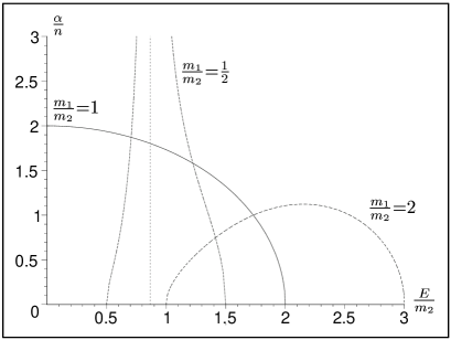
FIG. 1.: Plot of $\alpha/n$ versus $E/m_{2}$ for $n^{\prime}=0~{}(n=j+1/2)$ states of three different mass combinations, where $m_{1}$ is the fermion mass and $m_{2}$ is the boson mass.

We can, of course, evaluate and plot $\alpha(E)$ for any $n^{\prime},j$ state and any values of $m_{1},m_{2}$, using the analytic formula (8.7). However, it is instructive to outline the general behaviour of $E(\alpha)$, without specifying particular cases.

First of all, we recall that normalizable bound-state solutions (for which $\beta>0$) occur only for $|m_{1}-m_{2}|<E<m_{1}+m_{2}$. There are two branches to the solution $E(\alpha)$, much like for the scalar Yukawa model (1.1) described in the introduction. The upper branch, $E_{+}(\alpha)$, begins with the Balmer form $E_{+}=m_{1}+m_{2}-{1\over 2}{{m_{1}m_{2}}\over{m_{1}+m_{2}}}{{\alpha^{2}}\over{n^{2}}}+O(\alpha^{4})$ at low $\alpha$, then decreases monotonically towards a limiting value $E_{c}$. There is also a lower ‘unphysical’ branch that starts off as $E_{-}=|m_{1}-m_{2}|+{1\over 2}{{m_{1}m_{2}}\over{|m_{1}-m_{2}|}}{{\alpha^{2}}\over{n^{2}}}+O(\alpha^{4})$ for $m_{1}\neq m_{2}$ but as $E_{-}=m\alpha/n+O(\alpha^{3})$ for $m_{1}=m_{2}=m$, and increases monotonically towards $E_{c}$. The lower branch is not of Balmer form at low $\alpha$.

The qualitative behaviour of $E(\alpha)$ is different for the fermion-like case $m_{1}<m_{2}$ and the scalar-like case $m_{1}>m_{2}$. This is evident from the one-body limits, described below. For the fermion-like case there are bound state solutions for all values of $\alpha$, no matter how large. Indeed, as $\alpha\to\infty$, the upper branch $E_{+}(\alpha)$ approaches the value $E_{c}=\sqrt{m_{2}^{2}-m_{1}^{2}}$ from above, while the lower branch $E_{-}(\alpha)$ approaches this value from below. Thus, $E=E_{c}=\sqrt{m_{2}^{2}-m_{1}^{2}}$ is a horizontal asymptote of $E(\alpha)$ for the fermion-like cases.

In contrast, for scalar-like ($m_{1}/m_{2}>1$) cases, there are bound state solutions only for finite $\alpha\leq\alpha_{c}$, beyond which $E$ ceases to be real. The qualitative shape of $\alpha(E)$, is that of a distorted upper half-circle ($\alpha_{c}$ being the apex), reminiscent of the scalar Yukawa result (1.1). The critical point, $E_{c}(\alpha_{c})$ is the end-point for both branches for the scalar-like case. The critical value of $\alpha$ varies with $m_{1}/m_{2}>0$. We find that $\alpha_{c}/n>1$ for all scalar-like cases. The value $\alpha_{c}/n=1$ corresponds to the one-body Klein-Gordon limit ($m_{1}/m_{2}\to\infty$) for which $E_{c}-m_{1}=0$. For $n^{\prime}=0$ states, $\alpha_{c}$ lies in the domain $1\leq\alpha_{c}/n\leq 2$, where $\alpha_{c}/n=1$ corresponds to the equal-mass limit, $m_{2}=m_{1}$ (cf. Eq. (8.8)). For $n^{\prime}>0$ states, $\alpha_{c}/n$ generally increases with increasing $n^{\prime}$, and becomes arbitrarily large in the equal mass limit ($m_{1}/m_{2}\to 1$). We shall now discuss the limiting cases of the physical, upper branch of $E(\alpha)$ in some detail.

One mass is large and the other is small

First, we consider the one-body limits of $E_{+}(\alpha)$, which follow from (8.7) by making the substitutions $E=m_{a}(\varepsilon+1)$, where $\varepsilon=c_{1}\frac{m_{b}}{m_{a}}+c_{2}\left(\frac{m_{b}}{m_{a}}\right)^{2}+....$, and solving for the coefficients $c_{i}$ . For $m_{1}/m_{2}<1$ we obtain the fermion-like or Dirac limit:

$$E_{+}\left(\frac{m_{1}}{m_{2}}<1\right)=m_{2}+m_{1}\left[\sqrt{1-\frac{\alpha^{2}}{(n^{\prime}+\sqrt{\alpha^{2}+\kappa^{2}})^{2}}}\right.\qquad\qquad\qquad\qquad\qquad{}$$ (8.9)

$$\left.~{}~{}~{}~{}+~{}\frac{m_{1}}{m_{2}}\frac{\alpha^{2}}{2(n^{\prime}+\sqrt{\alpha^{2}+\kappa^{2}})^{2}}\left(1-\frac{2\alpha^{2}}{\sqrt{\alpha^{2}+\kappa^{2}}(n^{\prime}+\sqrt{\alpha^{2}+\kappa^{2}})}\right)+O\left(\left(\frac{m_{1}}{m_{2}}\right)^{2}\right)\right]$$ (8.10)

The first term in the square brackets is just the Dirac one body energy spectrum for a Coulombic potential (scalar coupling), and the second one gives the first order correction in $m_{1}/m_{2}$.

For $m_{2}/m_{1}<1$ the expansion yields the scalar or Klein-Gordon limit:

$$E_{+}\left(\frac{m_{2}}{m_{1}}<1\right)=m_{1}+m_{2}\left[\sqrt{1-\frac{\alpha^{2}}{n^{2}}}+\frac{m_{2}}{m_{1}}\frac{\alpha^{2}}{2n^{2}}+O\left(\left(\frac{m_{2}}{m_{1}}\right)^{2}\right)\right]$$ (8.11)

The first term in square brackets coincides with the Klein-Gordon one body energy spectrum in a Coulombic potential (scalar coupling), while the second gives the first order correction to it, in powers of $m_{2}/m_{1}$.

Expansion of $E$ in powers of the coupling constant

Next, we consider the expansion of $E_{+}(\alpha)$ in powers of $\alpha$. The result is

$$E_{+}(\alpha)=m_{1}+m_{2}-\frac{1}{2}m_{r}\frac{\alpha^{2}}{n^{2}}-\frac{1}{8}m_{r}\alpha^{4}\left[\left(1+\frac{m_{1}m_{2}}{(m_{1}+m_{2})^{2}}\right)\frac{1}{n^{4}}-4\frac{m_{2}^{2}}{(m_{1}+m_{2})^{2}}\frac{1}{n^{3}(j+\frac{1}{2})}\right]+O(\alpha^{6}),$$ (8.12)

where $\displaystyle n=n^{\prime}+j+\frac{1}{2}$ and $\displaystyle m_{r}=\frac{m_{1}m_{2}}{m_{1}+m_{2}}$. We obtain the expected non-relativistic Balmer result at O($\alpha^{2}$). The O($\alpha^{4}$) correction is not symmetric in $m_{1}$ and $m_{2}$ due to the different, fermionic and bosonic, nature of the particles. The one body limits of (8.12) have the required Dirac and Klein-Gordon forms, as can be seen from the expressions

$$E_{+}\left(\frac{m_{1}}{m_{2}}<1\right)=m_{2}+m_{1}\left[1-\frac{\alpha^{2}}{2n^{2}}-\frac{1}{8}\alpha^{4}\left(\frac{1}{n^{4}}-\frac{4}{n^{3}(j+\frac{1}{2})}\right)\right.\qquad\qquad{}$$ (8.13)

$$\left.+~{}\frac{m_{1}}{m_{2}}\left(\frac{\alpha^{2}}{2n^{2}}-\frac{3\alpha^{4}}{2n^{3}(j+\frac{1}{2})}\right)+O\left(\left(\frac{m_{1}}{m_{2}}\right)^{2}\!,~{}\alpha^{6}\right)\right],$$ (8.14)

$$E_{+}\left(\frac{m_{2}}{m_{1}}<1\right)=m_{1}+m_{2}\left[1-\frac{\alpha^{2}}{2n^{2}}-\frac{\alpha^{4}}{8n^{4}}+\frac{m_{2}}{m_{1}}\frac{\alpha^{2}}{2n^{2}}+O\left(\left(\frac{m_{2}}{m_{1}}\right)^{2}\!,\alpha^{6}\right)\right].$$ (8.15)

Note that (8.13) and (8.15) are the same as the expansions of Eqs. (8.9), (8.11) in powers of $\alpha$, as they ought to be.

IX Concluding remarks

We have studied two-particle systems in a model QFT, in which fermions of mass $m_{1}$ interact with bosons of mass $m_{2}$. The interaction is mediated by a real, scalar field of mass $\mu$ (the ‘chion’ field). The field equations were used to recast the Hamiltonian of the theory into a form in which the chion propagator appears directly in the interaction term. For the case where there is no decay, emission or absorption of real (physical) chions (i.e. only ’virtual’ chions), we obtain exact two-particle eigenstates of the Hamiltonian, using an unconventional ‘empty’ vacuum state, which is annihilated by both the positive and negative frequency parts of the particle-field operators.

The resulting relativistic two-particle wave equation, for the stationary states of the system, reduces to a pair of Dirac-like radial equations for the various $J^{P}$ states. These equations are shown to have the radial Schrödinger equation for the relative motion of the two particles as the non-relativistic limit, and the Dirac and Klein-Gordon equations (with scalar coupling) as the one-body limits. Analytic solutions for the two-body bound state eigenenergies (rest masses) are obtained for the massless chion exchange ($\mu=0$) case. The shape of the $E(\alpha)$, or $\alpha(E)$, curves, where $\alpha$ is the dimensionless coupling constant, is discussed for various mass combinations, $m_{1}/m_{2}$, and various $nJ^{P}$ states.

In the case of massive chion exchange ($\mu\neq 0$), the eigenvalues and eigenfunctions must be obtained numerically, which can be done easily by standard methods. We do not present such solutions in this paper. Also, we do not discuss the scattering-state solutions of the equations, though these can be worked out readily.

Lastly, we mention that $\cal N$-body eigenstates, where ${\cal N}\geq 3$, and the corresponding relativistic $\cal N$-body equations, can be worked out readily for the present model, as was shown for the purely scalar model in [3], and for QED in [15]. Such equations are much more complicated, since they possess all the complexity of relativistic many-body equations. We do not discuss the ${\cal N}\geq 3$ systems in this paper.

REFERENCES

• [1] G. C. Wick, Phys. Rev. 96, 1124 (1954).
• [2] R. E. Cutkosky, Phys. Rev. 96, 1135 (1954).
• [3] J. W. Darewych, Can. J. Phys. 76, 523 (1998).
• [4] M. Barham and J. Darewych, J. Phys. A 31, 3481 (1998).
• [5] E. Berezin, C. Itzykson and J. Zinn-Justin, Phys. Rev. D 1, 2349 (1970).
• [6] I. T. Todorov, in Properties of the Fundamental Interactions, A. Zichichi, ed. Editrice Compositori, Bologna, 1973 Part C, pp. 953-979.
• [7] V. I. Savrin and A. Yu. Troole, Theor. Math. Phys. 106, 333 (1996).
• [8] V. Tretyak and V. Shpytko, J. Phys. A 33, 5719 (2000).
• [9] B. Ding and J. Darewych, J Phys. G 26, 907 (2000).
• [10] T. Nieuwenhuis and J. A. Tjon, Phys. Rev. Lett. 77, 814 (1996).
• [11] J. D. Jackson, Classical Electrodynamics (John Wiley, New York, 1975).
• [12] A. O. Barut, Electrodynamics and Classical Theory of Fields and Particles (Dover, New York, 1980).
• [13] H. Feshbach and F. Villars, Rev. Mod. Phys. 30, 24 (1958).
• [14] e.g. J. D. Bjorken and S. D. Drell, Relativistic Quantum Fields, (McGraw-Hill, New York, 1965), p. 59.
• [15] J. W. Darewych, in Causality and Locality in Modern Physics, G. Hunter et al. (eds.), Kluwer, Dordrecht, 1998, pp. 333-244.