Space-time versus particle-hole symmetry in quantum Enskog equations

Abstract

The non-local scattering-in and -out integrals of the Enskog equation have reversed displacements of colliding particles reflecting that the -in and -out processes are conjugated by the space and time inversions. Generalisations of the Enskog equation to Fermi liquid systems are hindered by a request of the particle-hole symmetry which contradicts the reversed displacements. We resolve this problem with the help of the optical theorem. It is found that space-time and particle-hole symmetry can only be fulfilled simultaneously for the Bruckner-type of internal Pauli-blocking while the Feynman-Galitskii form allows only for particle-hole symmetry but not for space-time symmetry due to a stimulated emission of Bosons.

]

I Introduction

The formulation of kinetic theory of dense interacting Fermi gases beyond the Boltzmann equation (BE) is an ongoing task. For classical hard-sphere gas the main theoretical focus was on the statistical correlations resulting in the Enskog equation [1, 2, 3, 4, 5, 6, 7]. In contrast to the BE, the collision integral of the Enskog equation is non-local what takes into account that when two hard spheres collide, their centres are displaced by the sum of their radii. The particle scattered out of its free trajectory faces its collision partner in front, while the particle scattered in the new free trajectory leaves its partner behind. This is expressed by the opposite signs of non-local corrections in the scattering-out and -in integrals.

Various generalisations of the Enskog equation towards quantum systems [8, 9, 10, 11, 12, 13, 14] have been developed mostly in the last two decades. They offer numerous gradient corrections to the scattering integral which describe how the non-local character of collisions contributes to smooth perturbations. With a typical number of gradient corrections counted in tens, a comparison of the original Enskog equation with its generalisations was not possible.

The connection became more clear after Laloe, Nacher and Tastevin [13] recognized that some of obtained gradient corrections can be recast into effective fields and renormalizations of the mass of particles, i.e., these gradient corrections are linked to the Landau concept of quasiparticles. They also show that when the quasiparticle contributions are separated, all remaining gradient contributions are proportional to various derivatives of the scattering phase shift. These derivatives have natural link to the Wigner collision delay [15] which also describes the non-locality of collisions, although in the time not in the space.

A kinetic equation which combines the non-locality in time and space has been derived as the quasi-classical asymptotics of non-equilibrium Green’s functions [16, 17]. In [16] a backward resummation of the gradient expansion was introduced by which one obtains the scattering integral in a form reminding the Enskog equation: the gradient corrections are expressed as shifts of arguments in the initial (final) condition so that one can see how long the collision lasts and how far from each other are particles at the beginning (end) of a collision. Of course, the hard-sphere gas is a special case to which the theory applies. It turns out that the scattering-in is identical to the Enskog equation while the displacement of the scattering-out does not have the expected opposite sign. A careful inspection shows that this sign problem appears also within all earlier approaches [8, 9, 10, 11, 12, 13, 14].

The sign puzzle has two serious consequences for the applicability of the non-local kinetic equation. First, the Enskog equation corresponds to classical trajectories, therefore it can be numerically studied either with the Monte-Carlo simulation or by the so called molecular dynamics. The kinetic equations derived from the quantum statistics cannot be studied with these methods. Second, the Enskog equation yields the hydrodynamic Chapman-Enskog expansion in a straight and relatively simple manner [2] what allows one to identify the thermodynamic properties of the system. The symmetry between the scattering-in and -out is a very important prerequisite in separation of cancelling and conserving quantities. Without this symmetry, one can also derive conservation laws [12], however, an extensive application of physically non-transparent identities is necessary.

In this paper we show how the natural symmetry of the Enskog equation can be obtained within the quantum mechanical approach to the kinetic equation. In the next section we introduce the problem of symmetry in a naive manner using ad hoc kinetic equations for the Fermi liquid. In Section III we show that the non-local corrections for the Fermi liquid are linked to in-medium effects and provide an identity which allows one to achieve the Enskog form of non-local corrections. Section IV includes conclusions.

II Classical versus quantum collision

The problem with sign in the scattering-out follows from a difference between the classical and quantum approaches to collisions. One has to recognize that a realistic collision has a finite duration $\Delta_{t}$ and to compare these two approaches in the time picture.

A Pseudo-classical approach

The simplest model system on which one can illustrate both approaches is a homogeneous gas of particles which form short-living molecules, i.e., the system with a dominant resonant scattering [15]. Its kinetic equation reads

$${\partial f_{k}(t)\over\partial t}=\int PF_{k+p}(t)-\int Pf_{k}(t)f_{p}(t).$$ (1)

The last term is the scattering-out which describes that with the probability $P$ two particles form a molecule and thus a particles leaves the state of momentum $k$. The first term on the right hand side corresponds to the decay of the molecule into two particles, one of them achieves momentum $k$. The dependence of the distribution of molecules $F$ is also covered by the balance equation,

$${\partial F_{K}(t)\over\partial t}=\int Pf_{K-p}(t)f_{p}(t)-{F_{K}(t)\over\Delta_{t}}.$$ (2)

The last term describes the decay of molecules with lifetime $\Delta_{t}$, the first term on the right hand side their formation.

The balance equation (2) for molecules is solved by

$$F_{K}(t) = \int\limits^{\infty}_{0}d\tau{\rm e}^{-{\tau\over\Delta_{t}}}\int Pf_{K-p}(t-\tau)f_{p}(t-\tau)$$ (3)

$$\approx \int Pf_{K-p}(t-\Delta_{t})f_{p}(t-\Delta_{t}).$$ (4)

The second line is the gradient approximation which is sufficient for our discussion since all quantum approaches to the non-local kinetic equation are restricted to it. Using (4) in (1) one gets a kinetic equation,

$${\partial f_{k}(t)\over\partial t}=\int Pf_{k-q}(t\!-\!\Delta t)f_{p+q}(t\!-\!\Delta_{t})-\int Pf_{k}(t)f_{p}(t).$$ (5)

The scattering-in has a retarded initial condition reflecting that the molecule lives from $t-\Delta_{t}$ to $t$. The initial condition of the scattering-out is associated with time instant $t$, the corresponding molecule thus lives from $t$ to $t+\Delta_{t}$.

In dense Fermi systems, the final states of collisions might be occupied and the collision is then prohibited. Let us modify kinetic equation (5) by ad hoc Pauli blocking factors as introduced by Nordheim, Uehling and Uhlenbeck [18, 19]

$${\partial f_{k}(t)\over\partial t} = \int Pf_{k-q}(t-\Delta_{t})f_{p+q}(t-\Delta_{t})$$ (7)

$$\times\left(1-f_{k}(t)\right)\left(1-f_{p}(t)\right)$$

$$- \int Pf_{k}(t)f_{p}(t)$$ (9)

$$\times\left(1-f_{k-q}(t+\Delta_{t})\right)\left(1-f_{p+q}(t+\Delta_{t})\right).$$

The time arguments of the blocking factors, $1-f$, correspond to ends of time intervals during which the collision happens because the blocking is attributed to the final states.

B Quantum approach

One can see that the scattering-out of (9), obtained within pseudo-classical assumptions, requires the blocking factor at future time $t+\Delta_{t}$. The quantum approach, however, does not allow to look into future and treats the same process differently.

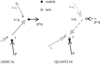
FIG. 1.: Scattering-out for classical and quantum concept of collisions.

In the quantum statistics, the scattering-out is described as a collision of two holes, see figure 1. In our simple model, two holes form a hole-molecule which also lives for $\Delta_{t}$. When this hole-molecule decays into two holes, these holes annihilate particles of corresponding momenta. Accordingly, the scattering-out is described by the hole-hole interaction during the time interval from $t-\Delta_{t}$ to $t$. An ad hoc kinetic equation corresponding to the quantum picture thus reads

$${\partial f_{k}(t)\over\partial t} = \int Pf_{k-q}(t-\Delta_{t})f_{p+q}(t-\Delta_{t})$$ (11)

$$\times\left(1-f_{k}(t)\right)\left(1-f_{p}(t)\right)$$

$$- \int Pf_{k}(t)f_{p}(t)$$ (13)

$$\times\left(1-f_{k-q}(t-\Delta_{t})\right)\left(1-f_{p+q}(t-\Delta_{t})\right).$$

Note that (13) differs from its pseudo-classical counterpart (9) by the sign of the non-local correction. This is the time-modification of the sign problem found for the quantum generalisations of the Enskog equation.

The above ad hoc implementations, Eq.’s (9) and (13), of the non-local corrections reveal a paradox: The space-time symmetry and the particle-hole symmetry lead to contradictory results. Indeed, equations (9) and (13) are different and for a general scattering rate $P$ they correspond to different thermodynamic properties of the system.

III In-medium effects

To resolve the paradox of symmetries, one has to take into account that the scattering rate $P$ itself is a function of the occupation, $P[f]$. This dependence represents an internal Pauli blocking of states during collisions, which is called in-medium effect in nuclear physics. In a heuristic manner one can indicate what kind of internal Pauli blocking is consistent with the Uehling-Uhlenbeck blocking of final states.

Since the scattering process lasts over the time interval from $t-\Delta_{t}$ to $t$, the mean value of $P$ equals its value at the centre time $P=P(t-{1\over 2}\Delta_{t})$, see [16, 17]. Comparing equations (9) and (13) we find that the two symmetries are consistent if

$$\int P\left(t-{1\over 2}\Delta_{t}\right)f_{k}(t)f_{p}(t)$$ (15)

$$~{}~{}~{}~{}~{}\times\left(1-f_{k-q}(t-\Delta_{t})\right)\left(1-f_{p+q}(t-\Delta_{t})\right)$$

$$= \int P\left(t+{1\over 2}\Delta_{t}\right)f_{k}(t)f_{p}(t)$$ (17)

$$~{}~{}~{}~{}~{}\times\left(1-f_{k-q}(t+\Delta_{t})\right)\left(1-f_{p+q}(t+\Delta_{t})\right).$$

Within the gradient approximation this condition reads

$$\int Pf_{k}f_{p}(1-f_{k-q})(1-f_{k-q})$$ (18)

$$\times\left({d\ln P\over dt}+2{d\over dt}\ln[(1-f_{k-q})(1-f_{p+q})]\right)=0.$$ (19)

¿From this equation we see that the space-time and particle-hole symmetries are consistent when the time dependence of in-medium effect is given by the Pauli blocking of the Bruckner type, $P[(1-f)(1-f)]$. According to this type of the Pauli blocking, the internal states of the short-living molecule exist only in the unoccupied phase space.

A Causality

The retarded scattering-out integral of Enskog type (9) is peculiar from the point of view of the causality. Since the scattering-out process ends at time $t+\Delta_{t}$, the scattered particles have to have available final state at this time. In other words, to determine whether the collision is allowed by the Pauli exclusion principle, one has to look into future. In such a way, the Pauli blocking seems to bring an anti-casual step.

In general, the causality of the perturbative expansion reflects the tendency of a many-body system to reach its equilibrium state. The anti-causal descriptions of the whole system is thus impossible because of the dissipative processes. Accordingly, we will take the causal expansion and the subsequent the particle-hole symmetry represented by (13) as well justified starting point.

The Enskog-type kinetic equation with the space-time symmetry of the scattering integral applies only under restrictive assumptions. The first assumption is that individual binary collisions are treated as if they were isolated from the rest of the system. The dynamics of the binary collision is then reversible and the causal and anti-causal expansions on the space-time scale of a single collision are equivalent. This assumption is met in all approaches to the kinetic equation except for the studies of the so called collisional broadening. The second assumption is that the internal Pauli blocking of collisions is of the Bruckner type. This point is discussed bellow.

All methods of the quantum statistics enforce the causality using backward propagation of holes instead of the forward propagation of particles into future. To link the space-time and particle-hole symmetries, we will use the optical theorem which allows us to reformulate the causal internal propagation during the collision into the anti-causal one.

In the algebraic notation of the double-time Green functions[20, 21, 22], the causality is reflected by the order of operators, ‘retarded–correlation–advanced’. The time cuts of the retarded and advanced operators restrict all time integrals to the past. The anti-causal expansion is then characterised by the reversed order, ‘advanced–correlation–retarded’. Without introducing unnecessary details, we can link the causal and anti-causal expansions using the identity for the scattering T-matrix,

$$T^{R}{\cal A}T^{A}=T^{A}{\cal A}T^{R}.$$ (20)

This identity represents two forms of the optical theorem, ${\rm Im}T=T^{R}{\cal A}T^{A}$ and ${\rm Im}T=T^{A}{\cal A}T^{R}$. Their derivations are enclosed in Appendix A.

The retarded/advanced T-matrix, $T^{R,A}$, describes an individual binary process [23]. The two-particle spectral function $\cal A$ includes the internal Pauli blocking. In this paper we discuss two particular approximations of the internal Pauli blocking, the Bruckner approximation,

$${\cal A}_{B}(t_{1},t_{2},k,p)\approx(1-f_{k})(1-f_{p}){\rm e}^{-i(\epsilon_{k}+\epsilon_{p})(t_{1}-t_{2})},$$ (21)

and the Galitskii-Feynman approximation,

$${\cal A}_{GF}(t_{1},t_{2},k,p)\approx(1-f_{k}-f_{p}){\rm e}^{-i(\epsilon_{k}+\epsilon_{p})(t_{1}-t_{2})}.$$ (22)

For both approximations we will derive kinetic equations with the space-time symmetry of the non-local scattering integral. We will see that the kinetic equation obtained within the Bruckner approximation has the pseudo-classical form (9), therefore it can be treated with numerical tools based on classical concept of trajectories. In contrast, the kinetic equation within the Galitskii-Feynman approximation includes a non-trivial term due to the stimulated emission of Bosons which essentially complicates its numerical treatment.

B Collision integral from Green functions

Let us first remind how the non-local scattering integrals relate to more general relations of the quantum statistics. We demonstrate it on the method of non-equilibrium Green’s functions. The scattering-in and -out integrals result from anti-commutators, $\{.,.\}$, of the Kadanoff and Baym (KB) equation [24, 25, 26]

$$\{G^{>},\Sigma^{<}\}\!-\!\{G^{<},\Sigma^{>}\} = \left\{G^{>},G^{>}\circ T^{R}(G^{<}G^{<})T^{A}\right\}$$ (23)

$$- \left\{G^{<},G^{<}\circ T^{R}(G^{>}G^{>})T^{A}\right\}.$$ (24)

Here, $G^{<}$ and $G^{>}$ are particle and hole correlation functions, the $\circ$ denotes that $G^{>,<}$ closes one loop of the two-particle function on its right hand side. The T-matrices and pairs of single-particle correlation functions, $(GG)$, obey standard two-particle operator products.

With respect to our treatment, it is sufficient to know that the particle correlation functions are proportional to the quasiparticle distribution, $G^{<}(t_{1},t_{2},k)\approx f_{k}{\rm e}^{-i\epsilon_{k}(t_{1}-t_{2})}$, therefore they represent the initial states of collisions. Similarly, the hole correlation functions are proportional to the hole distribution, $G^{>}(t_{1},t_{2},k)\approx(1-f_{k}){\rm e}^{-i\epsilon_{k}(t_{1}-t_{2})}$, therefore they describe the final states including their Pauli blocking.

According to initial and final states, the first and second terms of the right hand side of (LABEL:e7) can be interpreted as the scattering-in and -out integrals, respectively. Note that both scattering integrals are causal having order ‘retarded–correlation–advanced’ of the two-particle functions. In the same time, the scattering-in and -out integrals are linked via the particle-hole symmetry. One can see that upon the interchange of particles and holes, $>\longleftrightarrow<$, the first term changes to the second one and vice versa. Equation (LABEL:e7) is thus a precursor of (13).

Using the (extended) quasiparticle and quasi-classical approximations keeping gradients in the scattering integral of the KB equation, one obtains a non-local kinetic equation [16],

$${\partial f_{1}\over\partial t} + {\partial\epsilon_{1}\over\partial k}{\partial f_{1}\over\partial r}-{\partial\epsilon_{1}\over\partial r}{\partial f_{1}\over\partial k}$$ (26)

$$= \int P^{-}\ f_{3}^{-}f_{4}^{-}\bigl{(}1-f_{1}\bigr{)}\bigl{(}1-f_{2}^{-}\bigr{)}$$ (27)

$$- \int P^{-}\ \bigl{(}1-f_{3}^{-}\bigr{)}\bigl{(}1-f_{4}^{-}\bigr{)}f_{1}f_{2}^{-}.$$ (28)

Algebraic operations needed to arrive at (28) are rather extensive due to numerous gradient contributions to the scattering integrals. These gradient contributions are expressed via shifts of arguments as

$$f_{1} \equiv f(k,r,t)$$ (29)

$$f_{2}^{-} \equiv f(p,r\!-\!\Delta_{2},t)$$ (30)

$$f_{3}^{-} \equiv f(k\!-\!q\!-\!\Delta_{K},r\!-\!\Delta_{3},t\!-\!\Delta_{t})$$ (31)

$$f_{4}^{-} \equiv f(p\!+\!q\!-\!\Delta_{K},r\!-\!\Delta_{4},t\!-\!\Delta_{t}).$$ (32)

The differential cross section is proportional to the square of the amplitude of the T-matrix

$$P^{-}={dp\over(2\pi)^{3}}{dq\over(2\pi)^{3}}2\pi\delta\left(\epsilon_{1}+\epsilon_{2}^{-}-\epsilon_{3}^{-}-\epsilon_{4}^{-}-2\Delta_{E}\right)$$ (33)

$$\left|T\!\left(\!\epsilon_{1}\!+\!\epsilon_{2}^{-}\!-\!\Delta_{E},k-{\Delta_{K}\over 2},p-{\Delta_{K}\over 2},q,r-\Delta_{r},t-{\Delta_{t}\over 2}\right)\right|^{2}\!.$$ (34)

(35)

Arguments of quasiparticle energies, $\epsilon$’s, are identical with (32). All non-local corrections are given by derivatives of the scattering phase shift $\phi={\rm Im\ ln}T^{R}(\Omega,k,p,q,t,r)$ [16],

$$\Delta_{t} = {\partial\phi\over\partial\Omega},\ \ \ \Delta_{E}=-{1\over 2}{\partial\phi\over\partial t},\ \ \ \Delta_{K}={1\over 2}{\partial\phi\over\partial r},\ \ \ \Delta_{3}=-{\partial\phi\over\partial k},$$ (36)

$$\Delta_{2} = {\partial\phi\over\partial p}-{\partial\phi\over\partial q}-{\partial\phi\over\partial k},\ \ \ \ \ \ \ \ \ \ \Delta_{4}=-{\partial\phi\over\partial k}-{\partial\phi\over\partial q}.$$ (37)

A detail understanding of these numerous corrections to the scattering integral of the Boltzmann equation is not essential for our discussion. It is important to realize that the collision is of finite duration $\Delta_{t}$. During this time particles can gain momentum and energy, $\Delta_{K,E}$ due to the medium effect on the collision. Three displacements $\Delta_{2,3,4}$ correspond to initial and final positions of two colliding particles/holes.

The quasiparticle kinetic equation (28) covers three ingredients of the kinetic theory. First, the scattering integral includes medium effect on the scattering rate. Second, the scattering integrals are non-local in space and time. Third, the quasiparticle energy represents the momentum dependent mean field. With respect to included non-local corrections, it is important that the quasiparticle energy is defined from the pole of the propagator, not from the variation of the energy density. This difference has been discussed in [27]. The scattering-out of (28) is the particle-hole mirror of the scattering-in, accordingly it is not the space-time mirror found in the Enskog equation.

C Anti-causal collision integral

Our aim is to rearrange (28) so that it will include the scattering-out as the space-time mirror of the scattering-in, briefly, it will be the symmetry assumed by Enskog. It is advantageous to make this step already on the level of Green’s functions. Accordingly, we rearrange (LABEL:e7) so that its scattering-out part is written in terms of the anti-causal expansion.

Further progress depends on the approximation of the T-matrix. Let us first approximate the T-matrix by Bruckner’s reaction matrix for which the two-particle spectral function is ${\cal A}_{B}=(G^{>}G^{>})$. Formula (21) is the quasiparticle approximation of $(G^{>}G^{>})$. Using identity (20) in the second term of (LABEL:e7) one finds

$$\{G^{>},\Sigma^{<}\}\!-\!\{G^{<},\Sigma^{>}\} = \left\{G^{>},G^{>}\circ T^{R}(G^{<}G^{<})T^{A}\right\}$$ (38)

$$- \left\{G^{<},G^{<}\circ T^{A}(G^{>}G^{>})T^{R}\right\}.$$ (39)

Expression (LABEL:e9) has the desired explicit space-time symmetry in contrary to explicit particle-hole symmetry of (LABEL:e7). To see it in detail, we use (LABEL:e9) in the KB equation and employ the same steps as above (quasi-classical and quasiparticle approximations) to arrive at

$${\partial f_{1}\over\partial t} + {\partial\epsilon_{1}\over\partial k}{\partial f_{1}\over\partial r}-{\partial\epsilon_{1}\over\partial r}{\partial f_{1}\over\partial k}$$ (41)

$$= \int P^{-}\ f_{3}^{-}f_{4}^{-}\bigl{(}1-f_{1}\bigr{)}\bigl{(}1-f_{2}^{-}\bigr{)}$$ (42)

$$- \int P^{+}\ \bigl{(}1-f_{3}^{+}\bigr{)}\bigl{(}1-f_{4}^{+}\bigr{)}f_{1}f_{2}^{+}.$$ (43)

The shifts in the scattering-out have opposite signs,

$$f_{2}^{+} \equiv f(p,r\!+\!\Delta_{2},t)$$ (44)

$$f_{3}^{+} \equiv f(k\!-\!q\!+\!\Delta_{K},r\!+\!\Delta_{3},t\!+\!\Delta_{t})$$ (45)

$$f_{4}^{+} \equiv f(p\!+\!q\!+\!\Delta_{K},r\!+\!\Delta_{4},t\!+\!\Delta_{t}),$$ (46)

and similarly other ingredients denoted by superscript $+$.

It can be indicated why the change of the causal picture into the anti-causal one results in the flipped signs of all non-local corrections. First, one can use a formal argument. Writing the T-matrices as products of the amplitude and the phase, $T^{R}=|T|{\rm e}^{i\phi}$ and $T^{A}=|T|{\rm e}^{-i\phi}$, one can see that the interchange of retarded and advanced T-matrices merely flips the sign of the phase shift $\phi$. As all $\Delta$’s depend linearly on $\phi$, the gradient contributions of the anti-causal scattering-out have signs reversed with respect to the causal scattering-in. Second, there is a physical reason for the formal argument above. The amplitude of T-matrix represents a filter which selects a probability of individual channels. The factor of phase shift, ${\rm e}^{i\phi}$, is a unitary transformation which applies to individual components of the wave function in a manner which parallels the evolution operator. Products like ${\rm e}^{i\phi}\ldots{\rm e}^{-i\phi}$ correspond to transformation from one place to another, while ${\rm e}^{-i\phi}\ldots{\rm e}^{i\phi}$ to the backward one.

For the system of classical hard spheres, kinetic equation (43) reduces to the Enskog equation in the second order virial approximation. This limit includes three simplifications. First, the Pauli blocking factors vanish in the classical limit, $1-f\to 1$. Second, the quasiparticle energy reduces to the kinetic energy of free particles, $\epsilon_{1}\to{k^{2}\over 2m}$. For this limit it is important that the quasiparticle energy is defined from the pole of the propagator. Landau’s definition of $\epsilon$ based on the variation of the energy density yields a non-trivial quasiparticle energy even for the classical gas of hard spheres. Third, from the hard-sphere scattering phase shift, $\phi\to\pi-|q|D$, where $D$ is a diameter of colliding particles, one finds expected values of $\Delta$’s. The collision delay is zero, $\Delta_{t}\to 0$, there is no energy/momentum gain, $\Delta_{E,K}\to 0$, during collision none of particles move in space, $\Delta_{3}=0$ and $\Delta_{4}=\Delta_{2}$. The displacement of particles at the instant of collision is $\Delta_{2,4}=D$.

To summarise this chapter, we have shown that the space-time and the particle-hole symmetric forms of the non-local Boltzmann equation are equivalent if the scattering rate includes the in-medium effect on the level of the Bruckner reaction matrix.

D Comments on the Galitskii-Feynman T-matrix

The Bruckner approximation of the scattering rate has been quite common in earlier microscopic studies of the heavy ion reactions. Recently, most studies prefers the Galitskii-Feynman approximation [25, 26] for which the Pauli blocking of the internal states is controlled by the two-particle spectral function, ${\cal A}_{GF}=(G^{>}G^{>})-(G^{<}G^{<})$. Formula (22) is the quasiparticle approximation of ${\cal A}_{GF}$.

As mentioned, the Galitskii-Feynman approximation includes processes which go beyond the scope of naive kinetic equations. While terms $\propto(G^{>}G^{>})$ exclude correlation in the occupied phase space, terms $\propto(G^{<}G^{<})$ describe stimulated correlation by already existing pairs. These processes lead to the superconducting phase transition at low temperatures, therefore the system cannot be treated as a sum of single-particle excitations on the Fermi liquid ground state. Kinetic equations (9) and (13) are based on the idea of the simple Fermi liquid and do not include the stimulated processes.

Even with the stimulated processes included, the kinetic equation can be rearranged into the space-time symmetric form. Again, we make the rearrangement on the level of the Green functions. Scattering integrals (LABEL:e7) can be written so that their final states are consistent with the Galitskii-Feynman spectral function,

$$\{G^{>},\Sigma^{<}\}\!-\!\{G^{<},\Sigma^{>}\} =\left\{G^{>},G^{>}\circ T^{R}(G^{<}G^{<})T^{A}\right\}$$ (48)

$$-\left\{G^{<},G^{<}\circ T^{R}(G^{<}G^{<})T^{A}\right\}$$

$$-\bigl{\{}G^{<},G^{<}\circ T^{R}((G^{>}G^{>})-(G^{<}G^{<}))T^{A}\bigr{\}}.$$ (49)

The last term includes the Galitskii-Feynman two-particle spectral function and can be converted into the anti-causal picture. The causal/anti-causal forms of the resulting kinetic equation reads,

$${\partial f_{1}\over\partial t} + {\partial\epsilon_{1}\over\partial k}{\partial f_{1}\over\partial r}-{\partial\epsilon_{1}\over\partial r}{\partial f_{1}\over\partial k}$$ (51)

$$= \int P^{-}\ f_{3}^{-}f_{4}^{-}\bigl{(}1-f_{1}-f_{2}^{-}\bigr{)}$$ (52)

$$- \int P^{\mp}\ \bigl{(}1-f_{3}^{\mp}-f_{4}^{\mp}\bigr{)}f_{1}f_{2}^{\mp}.$$ (53)

The particle-hole symmetric form (with superscripts $-$) can be recast into (13) by a subtraction of stimulated processes, $\propto f_{3}^{-}f_{4}^{-}f_{1}f_{2}^{-}$ on both sides. In contrast, the space-time symmetric form (with superscripts $+$) cannot be recast to intuitive form (9) due to gradient contributions of stimulated processes, $\propto f_{3}^{+}f_{4}^{+}f_{1}f_{2}^{+}$. It is a pity, since the space-time symmetry is obligatory for numerical treatments based on the Monte-Carlo simulations. Equation (53) is not suited for the Monte-Carlo treatment because its scattering integrals can change their sign loosing their probabilistic interpretation. The Galitskii-Feynman type of kinetic equation (53) thus provides a more precise description of the system, but on cost of serious increase of difficulties of its numerical treatment. Because of these numerical problems, we discuss an implementation of symmetries only for the Bruckner approximation.

E Implementation of the symmetry in simulations

Equivalency of both forms of kinetic equation, (28) and (43), offers an important simplification of the numerical treatment. Expanding the scattering-out to the linear terms, one finds that amplitudes of anti-causal and causal corrections equal while signs are opposite. Since both forms are equivalent, the sum of gradient corrections to the scattering-out vanishes.

For highly inhomogeneous and/or fast evolving systems, like the nuclear matter in a heavy ion reaction, the Monte-Carlo simulation procedure spends a majority of the CPU time searching when and where a collision should be generated. Due to cancellation of gradient corrections to the scattering-out integral, this part of the simulation procedure remains the same as in the local approximation. All non-local corrections are included only after the collision event is selected. This scheme has been used in [28].

IV Conclusions

We have shown that the space-time symmetry of the non-local scattering integral becomes non-trivial if the Pauli exclusion principle has to be accounted for. Within the pseudo-classical form of the Pauli blocking represented by the hole distributions as introduced by Nordheim, Uehling and Uhlenbeck, the space-time symmetry and the particle-hole symmetry are consistent only if the scattering cross section includes in-medium effects of Bruckner type. Due their classical form, these non-local corrections are easily implemented into the Monte-Carlo simulations.

The more sophisticated approximation of Galitskii and Feynman includes the stimulated creation of the colliding pair. This process escapes the pseudo-classical interpretation of the scattering process what makes its implementation within the traditional Monte-Carlo simulation schemes impossible.

A Optical theorem

Identity (20) represents two alternative expressions of the anti-hermitian part of the T-matrix,

$$M={\rm Im}T=i(T^{R}-T^{A}).$$ (A1)

We derive this identity know as the optical theorem from the ladder approximation, which is the approximation used in the scattering integrals of the discussed kinetic equation.

The ladder approximation in the differential form reads,

$$T_{R,A}^{-1}=V-{\cal G}^{R,A}.$$ (A2)

Here, ${\cal G}^{R,A}$ are the two-particle propagators given by the time cut of the spectral function ${\cal A}=i({\cal G}^{R}-{\cal G}^{A})$. ¿From (A2) follows

$$i\left(T_{R}^{-1}-T_{A}^{-1}\right)=-{\cal A}.$$ (A3)

Multiplying (A1) by $T_{R}^{-1}$ one finds

$$T_{R}^{-1}M=i-iT_{R}^{-1}T_{A}.$$ (A4)

Finally, we express $T_{R}^{-1}$ from (A3),

$$T_{R}^{-1}=T_{A}^{-1}+i{\cal A},$$ (A5)

so that (A4) turns into the familiar optical theorem

$$M=T^{R}{\cal A}T^{A}.$$ (A6)

To obtain a less familiar anti-causal form of the optical theorem, we multiply (A1) by $T_{R}^{-1}$ from the right hand side,

$$MT_{R}^{-1}=i-iT_{A}T_{R}^{-1}.$$ (A7)

Now we substitute (A5) into (A7) what yields

$$M=T^{A}{\cal A}T^{R}.$$ (A8)

Comparing (A6) with (A8) one obtains identity (20).

REFERENCES

- [1] D. Enskog, in Kinetic theory, edited by S. Brush (Pergamon Press, New York, 1972), Vol. 3, orig.: K. Svenska Vet. Akad. Handl. 63(4) (1921).
- [2] S. Chapman and T. G. Cowling, The Mathematical Theory of Non-uniform Gases (Cambrigde University Press, Cambridge, 1990), third edition Chap. 16.
- [3] E. Cohen, Fundamental Problems in Statistical Mechanics (Nort-Holland, Amsterdam, 1962).
- [4] J. Weinstock, Phys. Rev. A 140, 460 (1965).
- [5] K. Kawasaki and I. Oppenheim, Phys. Rev. A 139, 1763 (1965).
- [6] J. R. Dorfman and E. G. Cohen, J. Math. Phys. 8, 282 (1967).
- [7] H. van Beijeren and M. H. Ernst, J. Stat. Phys. 21, 125 (1979).
- [8] K. Bärwinkel, Z. Naturforsch. a 24, 38 (1969).
- [9] F. Laloe, J. Phys. (Paris) 50, 1851 (1989).
- [10] D. Loos, J. Stat. Phys. 59, 691 (1990).
- [11] R. Snider, J. Stat. Phys. 61, 443 (1990).
- [12] M. de Haan, Physica A 164, 373 (1990); 165 224 (1990); 170 571 (1991).
- [13] P. J. Nacher, G. Tastevin and F. Laloe, Ann. Phys. (Leipzig) 48, 149 (1991); J. Phys. (Paris) I 1, 181 (1991).
- [14] T. Bornath, D. Kremp, W. D. Kraeft, and M. Schlanges, Phys. Rev. E 54, 3274 (1996).
- [15] P. Danielewicz and S. Pratt, Phys. Rev. C 53, 249 (1996).
- [16] V. Špička, P. Lipavský and K. Morawetz, Phys. Lett. A 240, 160 (1998).
- [17] P. Lipavský, K. Morawetz, and V. Špička, Annales de Physique 26,1 (2001), K. Morawetz, Habilitation University Rostock 1998.
- [18] L. W. Nordheim, Proc. Roy. Soc. (A) 119, 689 (1928).
- [19] E. A. Uehling and G. E. Uhlenbeck, Phys. Rev. 43, 552 (1933).
- [20] L. V. Keldysh, Zh. exper. teor. Fiz. 47, 1515 (1964).
- [21] D. C. Langreth and J. W. Wilkins, Phys. Rev. B 6, 3189 (1972).
- [22] L. Banyai and K. E. Sayed, Ann. Phys. 233, 165 (1994).
- [23] M. L. Goldberger and K. M. Watson, Collision Theory (Wiley, New York, 1964).
- [24] L. P. Kadanoff and G. Baym, Quantum Statistical Mechanics (Benjamin, New York, 1962).
- [25] P. Danielewicz, Ann. Phys. (NY) 152, 239 (1984).
- [26] W. Botermans and R. Malfliet, Phys.Rep. 198, 115 (1990).
- [27] P. Lipavský, V. Špička and K. Morawetz, Phys. Rev. E 59, R1291 (1999).
- [28] K. Morawetz et al., Phys. Rev. Lett. 82, 3767 (1999).