Ultra-relativistic heavy-ion collisions are complicated processes and their understanding requires a microscopic modelling of all stages: the formation, evolution and hadronisation of a strongly coupled plasma. If the energy density produced in the interaction volume is large enough, then the relevant degrees of freedom are quarks and gluons. The terrestrial recreation of this quark gluon plasma (QGP) will aid in understanding phenomena such as the big bang and compact stars.

Construction of the Relativistic Heavy Ion Collider at the Brookhaven National Laboratory is complete and the initial energy density: $\varepsilon\sim 10-100$ GeV/fm³, expected to be produced in the collisions at this facility is certainly sufficient for QGP formation. Experimentally there are two parameters that control the conditions produced: the beam/target properties and the impact parameter. Varying these parameters changes the nature of the debris measured in the detectors. Signals of QGP formation and information about its detailed properties are buried in that debris [1]. Predicting the signals and properties requires a microscopic understanding of the collisions, including their non-equilibrium aspects.

In the space-time evolution of a relativistic heavy ion collision the initial state is a system far from equilibrium. This system then evolves to form an equilibrated QGP, and the investigation of that evolution and the signals that characterise the process are an important contemporary aspect of QGP research.

The formation of a QGP is commonly described by two distinct mechanisms: the perturbative parton picture [2] and the string picture [3]. In the parton picture the colliding nuclei are visualised as clouds of partons and the plasma properties are generated by rapid, multiple, short-range parton-parton interactions. In the string picture the nuclei are imagined to pass through one another and stretch a flux tube between them as they separate, which decays via a nonperturbative particle-antiparticle production process. These approaches are complimentary and both have merits and limitations. Once the particles are produced the subsequent analysis proceeds using Monte-Carlo event generators [4, 5, 6].

Herein we employ the nonperturbative flux tube picture [7]. A flux tube is characterised by a linearly rising, confining quark-antiquark potential: $V_{q{\bar{q}}}(r)=\sigma\,r$. The string tension can be estimated in lattice simulations using static quark sources, which yields $\sigma\sim 4\Lambda_{\rm QCD}^{2}\sim 1\,$GeV$/$fm. This string tension can be viewed as a strong background field that destabilises the vacuum and the instability is corrected through particle-antiparticle production via a process akin to the Schwinger mechanism [8]. Figure 1 is an artist’s impression of this process.

Assuming a constant, uniform, Abelian field, $E$, one is able to derive an expression for the rate of particle production via this nonperturbative mechanism

$$S(p_{\perp})=\frac{dN}{dtdVd^{2}p_{\perp}}=|eE|\ln\bigg{[}1+\exp\bigg{(}-\frac{2\pi(m^{2}+p_{\perp}^{2})}{|eE|}\bigg{)}\bigg{]}.$$ (1)

where $m$ is the mass and $e$ the charge of the particles produced. It is plain from this equation that the production rate is enhanced with increasing electric field and suppressed for a large mass and/or transverse momentum.

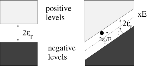
Figure 1: Left: For $E=0$ the vacuum is characterised by a completely filled negative-energy Dirac sea and an unoccupied positive-energy continuum, separated by a gap: $2\,\varepsilon_{\rm T}=2\,(m^{2}+p_{\perp}^{2})^{1/2}$. Right: Introducing a constant external field: $\vec{E}=\hat{e}_{x}E$, which is produced by a potential: $A^{0}=-E\vec{x}$, tilts the energy levels. In this case a particle in the negative-energy sea will tunnel through the gap with a probability $\sim\exp(-\pi\varepsilon_{T}^{2}/eE)$. Succeeding, it will be accelerated by the field in the $-x$-direction, while the hole it leaves behind will be accelerated in the opposite direction. The energy-level distortion is increased with increasing $E$ and hence so is the tunneling probability. $eE$ can be related to the flux-tube string-tension.

The production of charged particles leads naturally to an internal current. That current produces an electric field that increasingly screens and finally completely neutralises the background field so that particle creation stops. However, the current persists and the field associated with that internal current restarts the production process but now the field produced acts to retard and finally eliminate the current. …This is the back-reaction phenomenon and the natural consequences are time dependent fields and currents [9]. One observable and necessary consequence is plasma oscillations. Their properties, such as frequency and amplitude, depend on the initial strength of the background field and the frequency of interactions between the partons. It is clear that very frequent collisions will rapidly damp plasma oscillations and equilibrate the system.

The process we have described can be characterised by four distinct time-scales:

1. the quantum time, $\tau_{qu}$, which is set by the Compton wavelength of the particles produced and identifies the time-domain over which they can be localised/identified as “particles;”

2. the tunneling time, $\tau_{tu}$, which is inversely proportional to the flux tube field strength and describes the time between successive tunnelling events;

3. the plasma oscillation period, $\tau_{pl}$, which is also inversely proportional to field strength in the flux tube but is affected by other mechanisms as well;

4. and the collision period, $\tau_{coll}$, which is the mean time between two partonic collision events.

Each of the time-scales is important and the behaviour of the plasma depends on their relation to each other [10, 11]; e.g., non-Markovian (time-nonlocality) effects are dramatic if $\tau_{qu}\sim\tau_{tu}$. Herein we focus on the interplay of the larger time scales and consider a system for which $\tau_{pl}\sim\tau_{coll}$.

Particle creation is a natural outcome when solving QED in the presence of a strong external field and a formulation of this problem in terms of a kinetic equation is useful since, e.g., transport properties are easy to explore. The precise connection between this quantum kinetic equation and the mean field approximation in non-equilibrium quantum field theory [12] is not trivial and the derivation yields a kinetic equation that, importantly, is non-Markovian in character [13, 14, 15, 16].

The single particle distribution function is defined as the vacuum expectation value, in a time-dependent basis, of creation and annihilation operators for single particle states at time $t$ with three-momentum $\vec{p}$: $a^{\dagger}_{\vec{p}}(t)$, $a_{\vec{p}}(t)$; i.e.,

$$f(\vec{p},t):=\langle 0|a^{\dagger}_{\vec{p}}(t)\,a_{\vec{p}}(t)|0\rangle\,.$$ (2)

The evolution of this distribution function is described by the following quantum Vlasov equation:

$$\frac{df_{\pm}({\vec{P}},t)}{dt}=\frac{\partial f_{\pm}({\vec{P}},t)}{\partial t}+eE(t)\frac{\partial f_{\pm}({\vec{P}},t)}{\partial P_{\parallel}(t)}$$

$$= \frac{1}{2}{\cal W}_{\pm}(t)\int_{-\infty}^{t}dt^{\prime}{\cal W}_{\pm}(t^{\prime})\times[1\pm 2f_{\pm}({\vec{P}},t^{\prime})]\cos[x(t^{\prime},t)]+C_{\pm}({\vec{P}},t)\,,$$

where the lower [upper] sign corresponds to fermion [boson] pair creation, $C$ is a collision term and ${\cal W}_{\pm}$ are the transition amplitudes. The momentum is defined as ${\vec{P}}=(p_{1},p_{2},P_{\parallel}(t))$, with the longitudinal [kinetic] momentum $P_{\parallel}(t)=p_{3}-eA(t)$.

We approximate the collision-induced background field by an external, time-dependent, spatially homogeneous vector potential: $A_{\mu}$, in Coulomb gauge: $A_{0}=0$, taken to define the $z$-axis: ${\vec{A}}=(0,0,A(t))$. The corresponding electric field, also along the $z$-axis, is

$$E(t)=-{\dot{A}}(t)=-\frac{dA(t)}{dt}\,.$$ (4)

For fermions [13, 15] and bosons [11, 15] the transition amplitudes are

$${\cal W}_{-}(t)=\frac{eE(t)\varepsilon_{\perp}}{\omega^{2}(t)}\,,\;\;{\cal W}_{+}(t)=\frac{eE(t)P_{\parallel}(t)}{\omega^{2}(t)}\,,$$ (5)

where the transverse energy $\varepsilon_{\perp}=\sqrt{m^{2}+\vec{p}_{\perp}^{\,2}}$, ${\vec{p}}_{\perp}=(p_{1},p_{2})$, and $\omega(t)=\sqrt{\varepsilon_{\perp}^{2}+P_{\parallel}^{2}(t)}$ is the total energy. In Eq. (S0.Ex1),

$$x(t^{\prime},t)=2[\Theta(t)-\Theta(t^{\prime})]\,,\;\;\Theta(t)=\int^{t}_{-\infty}dt^{\prime}\omega(t^{\prime})\,,$$ (6)

is the dynamical phase difference.

The time dependence of the electric field is obtained by solving the Maxwell equation

$$-{\ddot{A}}^{\pm}(t)={\dot{E}}^{\pm}(t)=-j^{ex}(t)-j_{cond}(t)-j_{pol}(t)$$ (7)

where the three components of the current are: the external current generated, obviously, by the external field; the conduction current

$$j_{cond}(t)=g_{\pm}e\int\!\frac{d^{3}p}{(2\pi)^{3}}\,\frac{P_{\parallel}(t)}{\omega({\vec{P}},t)}f_{\pm}({\vec{P}},t)\,,$$ (8)

associated with the collective motion of the charged particles; and the polarisation current

$$j_{pol}(t)=g_{\pm}e\int\!\!\frac{d^{3}P}{(2\pi)^{3}}\frac{P_{\parallel}(t)}{\omega({\vec{P}},t)}\left[\frac{S({\vec{P}},t)}{{\cal W}_{\pm}({\vec{P}},t)}-\frac{e\,\dot{E}^{\pm}(t)\,P_{\parallel}(t)}{8\,\omega^{4}(\vec{P},t)}\right]\bigg{(}\frac{\epsilon_{\perp}}{P_{\parallel}(t)}\bigg{)}^{g_{\pm}-1}\!\!\!,$$ (9)

which is proportional to the production rate. Here $g_{-}=2$, $g_{+}=1$ and all fields and charges are understood to be fully renormalised, which has a particular impact on the polarisation current [17].

We mimic a relativistic heavy ion collision by using an impulse profile for the external field

$$E_{ex}=-\frac{A_{0}}{b}{\rm sech}^{2}(t/b)\,,$$ (10)

which is our two-parameter model input: the width $b$ and the amplitude $A_{0}$ are chosen so that the initial conditions are comparable to typical/anticipated experimental values. This is the seed in a solution of the coupled system of Eqs. (S0.Ex1) and (7)–(9), and in Fig. 2 we illustrate the result for the electric field in the absence of collisions.

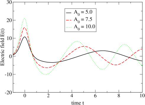
Figure 2: Time evolution of the fermion’s electric field obtained with three different initial field strengths. The amplitude and frequency of the plasma oscillations increases with an increase in the strength of the external impulse field, Eq. (10). The reference time-scale is the lifetime $b$ of the impulse current. (The field and time are given in arbitrary units, and $b=0.5$.)

The qualitative features are obvious and easy to understand. The external impulse (the collision) is evident: the portion of the curve roughly symmetric about $t=0$, where the field assumes its maximum value $A_{0}/b$. It produces charged particles and accelerates them, producing a positive current and an associated field that continues to oppose the external field until the net field vanishes. At that time particle production ceases and the current reaches a maximum value. However, the external field is dying away: it’s lifetime is $t\sim 0.5$, so that the part of the electric field due to the particles’ own motion quickly finds itself too strong. The excess of field strength begins to produce particles. It accelerates these in the opposite direction to the particles generating the existing current whilst simultaneously decelerating the particles in that current. That continues until the particle current vanishes, at which point the net field has acquired its largest negative value. Particle production continues and with that a negative net current appears and grows. … Now a pattern akin to that of an undamped harmonic oscillator has appeared. In the absence of other effects, such as collisions, it continues in a steady state with the magnitude and period of the plasma oscillations determined by the two model parameters that characterise the collision.

The quantum kinetic equation, Eq. (S0.Ex1), describes a system far from equilibrium and therefore any realistic collision term $C$ valid shortly after the impact must be expected to have a very complex form. However, as Fig. 2 illustrates, the evolution at not-so-much later times is determined by the properties of the particles produced and not by the violent nonequilibrium effects of the collision. This observation suggests that the parton plasma can be treated as a quasi-equilibrium system and that the effects of collisions can be represented via a relaxation time approximation [17, 18, 19, 20, 21]:

$$C({\vec{p}},t)=\frac{1}{\tau(t)}[f_{-}^{eq}({\vec{p}},t)-f({\vec{p}},t)]\,,$$ (11)

with $\tau(t)$ an in general time-dependent “relaxation time” (although we use a constant value $\tau(t)=\tau_{r}$ in the calculations reported herein) where

$$f_{-}^{eq}({\vec{p}},T(t))=\left[\exp\left(\frac{p_{\nu}u^{\nu}(t)}{T(t)}\right)+1\right]^{-1}$$ (12)

is the quasi-equilibrium distribution function for fermions. Here $T(t)$ is a local-temperature and $u^{\nu}(t)$, $u^{2}=1$, is a hydrodynamical velocity [20]. (With our geometry, $u^{\nu}(t)=(1,0,0,v(t))/[1-v^{2}(t)]^{1/2}$.)

Our definition of quasi-equilibrium is to require that at each $t$ the energy and momentum density in the evolving plasma are the same as those in an equilibrated plasma; i.e., we require that

$$\epsilon_{f}(t)=\epsilon^{eq}(t)\,,\;\vec{p}_{f}(t)=\vec{p}^{\,eq}(t)$$ (13)

where, as one would expect,

$$\epsilon^{eq}(t)=\int\frac{d^{3}p}{(2\pi)^{3}}\,\omega({\vec{p}},t)\,f_{-}^{eq}({\vec{p}},t)\,,\;\vec{p}^{\,eq}(t)=\int\frac{d^{3}p}{(2\pi)^{3}}\,\vec{p}(t)\,f_{-}^{eq}({\vec{p}},t)\,,$$ (14)

and

$$\epsilon_{f}(t) = \int\frac{d^{3}p}{(2\pi)^{3}}\,\omega({\vec{p}},t)\left[f_{-}({\vec{p}},t)-z_{f_{-}}({\vec{p}},t)\right]\,,$$ (15)

$$\vec{p}_{f}(t) = \int\frac{d^{3}p}{(2\pi)^{3}}\,\vec{p}(t)\left[f_{-}({\vec{p}},t)-z_{f_{-}}({\vec{p}},t)\right]\,,$$ (16)

where

$$z_{f_{-}}({\vec{p}},t)=\bigg{(}\frac{e\varepsilon_{\perp}}{4\omega^{3}}\bigg{)}^{2}\bigg{[}E(t)^{2}-\frac{e^{-2t/\tau_{r}}}{\tau_{r}}\int\limits_{-\infty}^{t}dt^{\prime}E(t^{\prime})^{2}e^{2t^{\prime}/\tau_{r}}\bigg{]}$$ (17)

is a regularising counterterm. Adding Eqs. (13) to the system of coupled equations embeds implicit equations for the temperature profile, $T(t)$, and collective velocity, $v(t)$.

Solving the complete set of coupled equations is a straightforward but time consuming exercise. For the present illustration we employ the minor simplification of assuming that the equilibrium energy density is that of a two-flavour, massless, free-quark gas; i.e.,

$$\epsilon^{eq}(T(t))=\frac{7\pi^{2}}{10}T^{4}(t)$$ (18)

and then proceed.

The solution obtained for the electric field using the impulse profile, Eq. (10), is depicted Fig. 3. Here the behaviour is analogous to that of a damped oscillator: the frequency and amplitude of the plasma oscillations diminishes with increasing collision frequency, $1/\tau_{r}$ (friction).

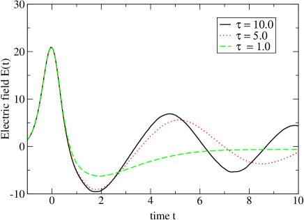
Figure 3: Time evolution of the electric field for three different relaxation times. As one would anticipate, collisions damp the plasma oscillations: their frequency and amplitude decreases with decreasing relaxation time. Solution obtained using the impulse profile, Eq. (10), with $A_{0}=10$, $b=0.5$. The field and the time are given in arbitrary units.

In the examples presented hitherto we have employed a constant fermion mass. However, in QCD the dressed-quark mass is momentum-dependent [22, 23] and that momentum-dependence is significant when $m_{0}\mathrel{\hbox to0.0pt{\lower 4.0pt\hbox{\hskip 0.0pt$\sim$}\hss}\raise 1.0pt\hbox{$<$}}\Lambda_{\rm QCD}$, where $m_{0}$ is the current-quark mass. That can be illustrated using a simple, instantaneous Dyson-Schwinger equation model of QCD, introduced in Ref. [24], which yields the following pair of coupled equations for the scalar functions in the dressed-quark propagator: $S(p)=1/[i\gamma\cdot p\,A(\vec{p}^{\,2})+B(\vec{p}^{\,2})]$,

$$B({\vec{p}},t) = m_{0}+\eta\frac{B({\vec{p}},t)}{\sqrt{{\vec{p}}^{2}\,A^{2}({\vec{p}},t)+B^{2}({\vec{p}},t)}}\,(1-2f_{-}(\vec{p},t))\,,$$ (19)

$$A({\vec{p}},t) = \frac{2B({\vec{p}},t)}{m_{0}+B({\vec{p}},t)}\,,$$ (20)

where $\eta$ is the model’s mass scale. In this preliminary, illustrative calculation we discard the distribution function in Eq. (19).

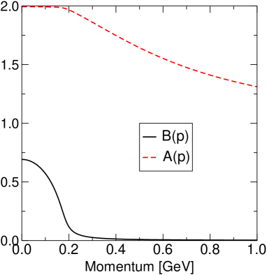
Figure 4: The scalar functions characterising a dressed-$u$-quark propagator, as function of momentum, obtained using the simple DSE model introduced in Ref. [24], see Eqs. (19), (20). We plot the functions as obtained at $T=T_{c}=0.17\,$GeV, which is the critical temperature for deconfinement in the model [25].

The solution obtained using a current-quark mass $m_{0}=5\,$MeV and with $\eta=1.33\,$GeV is depicted in Fig. 4. This value of the mass-scale parameter can be compared with the potential energy in a QCD string at the confinement distance, $V_{q\bar{q}}(r=1\,\mbox{fm})=\sigma r\simeq(2\Lambda_{\rm QCD})^{2}(1/\Lambda_{\rm QCD})=4\Lambda_{\rm QCD}\sim 1.0\,$GeV. The dressed-quark mass function is $m(\vec{p}^{\,2},T)=B(\vec{p}^{\,2},T)/A(\vec{p}^{\,2},T)$, and $m(0,T)$ provides a practical estimate of the $T$-dependent constituent-quark mass [26]: in this example $m(0,T_{c})\approx 0.35\,$GeV.

In our flux tube model for particle production we produce fermions with different momenta and following this discussion it is clear that the effective mass of the particles produced must be different for each momentum. That will affect the production and evolution of the plasma. To illustrate that we have repeated the last calculation using $m(p)$ wherever the particle mass appears in the system of coupled equations for the single particle distribution function. The effect on the electric field is depicted in Fig. 5, wherein it is evident that the plasma oscillation frequency is increased when the momentum-dependent mass is used because many of the particles produced are now lighter than the reference mass and hence respond more quickly to changes in the electric field.

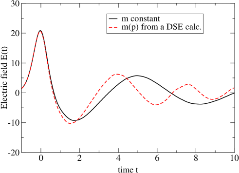
Figure 5: Electric field as function of time for $A_{0}=10.0$, $\tau=5.0$, $b=0.5$. We compare the results obtained using particles produced with a constant mass, $m=1$, with those obtained when the mass is momentum-dependent. For illustrative simplicity, we use the profile in Fig. 4 but normalised such that, $m(0)=m$. The mass-scale is arbitrary.

We have sketched a quantum Vlasov equation approach to the study of particle creation in strong fields. Using a simple model to mimic a relativistic heavy ion collision, we solved for the single particle distribution function and the associated particle currents and electric fields. Plasma oscillations are a necessary feature of all such studies. We illustrated that the oscillation frequency depends on: the initial energy density reached in the collision, it increases with increasing energy density; and the particle-particle collision probability, it decreases as this probability increases; and that it is sensitive to the necessary momentum-dependence of dressed-particle mass functions. The response in each case is easy to understand intuitively and that is a strength of the Vlasov equation approach.

Acknowledgments. A.V.P. is grateful for financial support provided by the Deutsche Forschungsgemeinschaft under project no. 436 RUS $17/102/00$. This work was supported by the US Department of Energy, Nuclear Physics Division, under contract no. W-31-109-ENG-38; the US National Science Foundation under grant no. INT-9603385; and benefited from the resources of the National Energy Research Scientific Computing Center.

References

- [1] S.A. Bass, M. Gyulassy, H. Stöcker and W. Greiner, J. Phys. G G 25 (1999) R1; S. Scherer et al., Prog. Part. Nucl. Phys. 42 (1999) 279; U. Heinz and M. Jacob, “Evidence for a new state of matter: An assessment of the results from the CERN lead beam programme,” nucl-th/0002042.
- [2] L.V. Gribov and M.G. Ryskin, Phys. Rept. 189 (1990) 29; T.S. Biro, C. Gong, B. Müller and A. Trayanov, Int. J. Mod. Phys. C 5 (1994) 113; L. McLerran and R. Venugopalan, Phys.Rev. D 49 (1994) 2233; ibid 3352.
- [3] B. Andersson, G. Gustafson, G. Ingelman and T. Sjöstrand, Phys. Rept. 97 (1983) 33.
- [4] X. Wang and M. Gyulassy, Phys. Rev. D 44 (1991) 3501.
- [5] K. Geiger, Phys. Rept. 258 (1995) 237.
- [6] B. Andersson, G. Gustafson and B. Nilsson-Almquist, Nucl. Phys. B 281 (1987) 289; K. Werner, Phys. Rept. 232 (1993) 87; S.A. Bass et al., Prog. Part. Nucl. Phys. 41 (1998) 225.
- [7] A. Casher, H. Neuberger and S. Nussinov, Phys. Rev. D 20 (1979) 179.
- [8] J. Schwinger, Phys. Rev. 82 664 (1951) 664; W. Greiner, B. Müller, and J. Rafelski, Quantum Electrodynamics of Strong Fields (Springer-Verlag, Berlin, 1985).
- [9] Y. Kluger, J.M. Eisenberg, B. Svetitsky, F. Cooper and E. Mottola, Phys. Rev. Lett. 67 (1991) 2427; K. Kajantie and T. Matsui, Phys. Lett. B 164 (1985) 373; A. Bialas, W. Czyż, A. Dyrek and W. Florkowski, Nucl. Phys. B 296 (1988) 611. M.A. Lampert and B. Svetitsky, Phys. Rev. D 61 (2000) 034011.
- [10] C.D. Roberts and S.M. Schmidt, Prog. Part. Nucl. Phys. 45 (2000) S1.
- [11] Y. Kluger, E. Mottola, and J.M. Eisenberg, Phys. Rev. D 58 (1998) 125015.
- [12] F. Cooper and E. Mottola, Phys. Rev. D 36 (1987) 3114; ibid D 40 (1989) 456; M. Herrmann and J. Knoll, Phys. Lett. B 234 (1990) 437; D. Boyanovsky, H.J. de Vega, R. Holman, D.S. Lee and A. Singh, Phys. Rev. D 51 (1995) 4419; W. Dittrich and H. Gies, Springer Tracts Mod. Phys. 166 (2000) 1.
- [13] J. Rau and B. Müller, Phys. Rept. 272 (1996) 1.
- [14] S.M. Schmidt D. Blaschke, G. Röpke, S.A. Smolyansky, A.V. Prozorkevich and V.D. Toneev, Int. J. Mod. Phys. E 7 (1998) 709.
- [15] S.A. Smolyansky, G. Röpke, S.M. Schmidt, D. Blaschke, V.D. Toneev and A.V. Prozorkevich, hep-ph/9712377; S.M. Schmidt, A.V. Prozorkevich, and S.A. Smolyansky, Creation of boson and fermion pairs in strong fields, Proceedings ’V. Workshop on Nonequilibrium Physics at Short Time Scales’, April 27-30, 1998, hep-ph/9809233.
- [16] S.M. Schmidt, D. Blaschke, G. Röpke, A.V. Prozorkevich, S.A. Smolyansky and V.D. Toneev, Phys. Rev. D 59 (1999) 094005.
- [17] J.C.R. Bloch, V.A. Mizerny, A.V. Prozorkevich, C.D. Roberts, S.M. Schmidt, S.A. Smolyansky, D.V. Vinnik, Phys. Rev. D 60 (1999) 116011.
- [18] J.C.R. Bloch, C.D. Roberts and S.M. Schmidt, Phys. Rev. D 61 (2000) 117502.
- [19] J.M. Eisenberg, Found. Phys. 27 (1997) 1213.
- [20] N.K. Glendenning and T. Matsui, Phys. Lett. B 141 (1984) 419; M. Gyulassy and T. Matsui, Phys. Rev. D 29 (1984) 419; K. Kajantie, R. Raitio and P.V. Ruuskanen, Nucl. Phys. B 222 (1983) 152; G. Baym, B.L. Friman, J.P. Blaizot, M. Soyeur and W. Czyż, Nucl. Phys. A 407 (1983) 541.
- [21] G.C. Nayak, A. Dumitru, L. McLerran and W. Greiner, “Equilibration of the gluon-minijet plasma at RHIC and LHC,” hep-ph/0001202.
- [22] C.D. Roberts and A.G. Williams, Prog. Part. Nucl. Phys. 33 (1994) 477.
- [23] J. I. Skullerud and A. G. Williams, hep-lat/0007028.
- [24] C.D. Roberts and S.M. Schmidt, “Temperature, chemical potential and the -meson,” in Proc. of the International Workshop XXVIII on Gross Properties of Nuclei and Nuclear Excitations, edited by M. Buballa, W. Nörenberg, B.-J. Schaefer and J. Wambach (GSI mbH, Darmstadt, 2000), pp. 185-191.
- [25] D. Blaschke, C.D. Roberts and S.M. Schmidt, Phys. Lett. B 425 (1998) 232.
- [26] P. Maris and C.D. Roberts, Phys. Rev. C 56 (1997) 3369.