Toy Model for Pion Production in Nucleon-Nucleon Collisions

Abstract

We develop a toy model of pion production in nucleon-nucleon collisions that reproduces some of the features of the chiral Lagrangian calculations. We calculate the production amplitude and examine some common approximations.

NT@UW–00–24

RBRC–142

KRL MAP–273

I Introduction

Interest in studies of pion production in nucleon-nucleon collisions at energies near threshold has been re-vitalized by the appearance of excellent high quality data [1]. The fact that low- and medium-energy strong interactions are controlled by chiral symmetry led to an early hope that chiral effective theories could be used to analyze these processes and achieve a fundamental understanding of the production process. Indeed, there are now tree level calculations [2, 3, 4, 5, 6, 7] and even loop calculations [8, 9, 10] available in the literature [11]. The early excitement was quickly abated by the realization that proper evaluation involves surmounting several severe difficulties, which are caused by the high momentum transfer nature of this threshold process. The initial relative momentum between the two nucleons must be at least $p_{i}=\sqrt{m_{\pi}M_{N}}$. This means that the chiral expansion is in terms of powers of $\sqrt{m_{\pi}/M_{N}}$ instead of $m_{\pi}/M_{N}$ [2, 12],which complicates carrying out the expansion and verifying its convergence. However, issues of convergence are not the focus of the present work. Instead, we address some technical questions which arise during the evaluation of the relevant matrix elements.

It is worthwhile to discuss some general features of the pion production process before describing our specific technical issues. Pion production occurs when the mutual interactions between two nucleons cause a real pion to be emitted. The leading term is one in which the initial and final state two-nucleon ($NN$) scattering allow a pion to be emitted by a single nucleon emission. The next tree level contribution occurs when a virtual pion of four-momentum $q$ produced by one nucleon is knocked on to its mass shell by an interaction with the second nucleon. This is the so-called re-scattering diagram. This process typically occurs accompanied by low-momentum-transfer initial and/or final state interactions. The evaluation of these diagrams, including the case when the pion exchanged between the two nucleons may be on shell, is our focus. Our strategy will be to introduce a toy model, which is simple enough to allow the exact evaluation of certain amplitudes. Then we may assess various approximations by comparing the resulting amplitudes to the exact results.

In general, one could obtain the necessary transition matrix elements by evaluating the relevant Feynman diagrams. However, the initial and final state interactions are accurately treated using an appropriate $NN$ potential within a three-dimensional Schrödinger equation formulation. Thus one needs to obtain a three-dimensional formulation from the more general Feynman procedure. This has been done in an ad hoc manner in Refs. [2, 3, 6, 7, 8]: one guesses the energy dependence of the virtual pion-nucleon ($\pi N$) interaction, and uses a Klein-Gordon propagator for the pion propagator. However, there is a general method to derive a three-dimensional theory which is equivalent to the Feynman diagram approach, namely the method of considering all the time-ordered diagrams —the use of time-ordered perturbation theory (TOPT). In this formulation, one finds only $NN$, $\pi NN$ and $\pi\pi NN$ propagators in the tree-level re-scattering diagrams. The Feynman Klein-Gordon pion propagator does not appear explicitly. Thus our first focus is the appropriate propagator. In particular, we will compare different prescriptions used in the literature with the exact result derived in the toy model.

Another issue to be addressed is that of the proper choice of the energy variable $q_{0}$ of the exchanged pion. The value of $q_{0}$ is critical because the chiral $\pi N$ interaction includes seagull vertices involving $\partial_{0}\pi$, such as the isovector Weinberg-Tomozawa interaction $N^{\dagger}\tau N\cdot(\pi\times\partial_{0}\pi)$ and the isoscalar $N^{\dagger}N(\partial_{0}\pi)^{2}$. In case of the isoscalar re-scattering, which is most relevant for threshold $\pi^{0}$ production, this seagull term is $\propto q_{0}m_{\pi}$. Its actual size is crucial: for on-shell $\pi N$ scattering at threshold ($q_{0}=m_{\pi}$) there is an almost complete cancelation of different, individually large terms leading to a very small $\pi N$ isoscalar scattering length [13]. If one moves away from the threshold or the on-shell $\pi N$ kinematics, however, this cancelation gets less and less effective. Thus the numerical value of the isoscalar re-scattering term is very sensitive to the details of the individual terms. Note that, because of the Weinberg-Tomozawa term, the proper choice for $q_{0}$ is also relevant for the isovector re-scattering that contributes to charged pion production.

If one simply evaluates the re-scattering diagram at threshold, neglecting initial- and final-state interactions, it is clear that $q_{0}=m_{\pi}/2$. Keeping this value fixed also when including the distortions leads to an amplitude that is opposite in sign to the on-shell scattering amplitude, and interferes destructively with the single-nucleon emission term [2, 3]. This choice for $q_{0}$ in combination with the use of the Klein–Gordon propagator for the pion will be called fixed kinematics approximation in what follows. Refs. [2, 3] found that the computed cross sections fell well below the data, unless many other even less-well constrained terms are included [6]. However, once the nucleons are no longer on shell, there are other prescriptions in the literature for choosing $q_{0}$. In a Feynman diagram this is the difference between the $0$th component of the nucleon four-momentum before and after pion emission. Thus one might find it natural to set $q_{0}$ equal to this difference in energies. Using this energy difference prescription in the distorted wave Born approximation (DWBA) calculation of pion production leads to a re-scattering diagram which also has a sign opposite to that of the single nucleon term, but which is about three times larger in magnitude[4]. As a result, one can reproduce the magnitude of the total cross section using only the re-scattering diagram. This energy prescription will be called $(E-E^{\prime})$ approximation below.

In addition, having the toy model at hand, we also want to study the importance of terms that go beyond the DWBA, namely the so-called stretched boxes (c.f. Fig.1, diagrams F3 and F4). These necessarily occur in the three-dimensional framework and represent diagrams where there is no two nucleon cut.

Note that the questions under investigation affect not only chiral perturbation theory calculations, but also more phenomenological approaches. For example, Ref. [14] used the $(E-E^{\prime})$ prescription for the pion re-scattering when investigating the influence of nucleon resonances on the production process. In the so-called Jülich model [15] the full TOPT propagator was used, but with its energy fixed to the production threshold. Thus, a clarification of these formal issues is necessary before one can draw conclusions about the physics of the process. This paper is meant to be a step in that direction.

It is important to realize that one can not resolve the ambiguity in the choice of $q_{0}$ or the proper $\pi NN$ propagator (in what follows this quantity will sometimes in a somewhat sloppy way be called “pion propagator”) by appealing to data. These are questions about the theory which arise due to the manner the DWBA procedure was implemented [2, 3, 4, 8]. Furthermore, the slow convergence of the momentum expansion requires one to resolve these difficulties before evaluating loop diagrams.

One needs to construct an ab initio theory of pion production. Doing this for the realistic case requires that one considers several important features including i) the spin and isospin of the two-nucleon system; ii) the Goldstone boson nature of the pion as an odd parity system degenerate with the vacuum; and iii) a realistic $NN$ potential. However, none of these features affects directly the questions which we want to examine. Therefore it is appropriate to construct a toy model which is simple enough to evaluate so that exact answers can be obtained. Then we can consider the various choices for $q_{0}$ and for the “pion propagators” as testable approximations. In the section II we formulate our toy model, and examine the various approximations for final- and initial-state interactions in sections III and IV, respectively. Our conclusions are summarized in section V.

II The Toy Model

The first step is to construct the necessary solvable model. Therefore:

i) We consider the production of a scalar “pion” field which has a Yukawa coupling with the nucleons. (We shall leave out the quotes around pion in the following text.)

ii) We include two nucleon fields, or, alternatively, treat nucleons as distinguishable. As a consequence, we need only include pion emission from one nucleon, but not the symmetric term where the pion is emitted from the other nucleon. We do not have to worry about several spin-isospin channels, and respective projections. The simplicity of the model is retained by allowing the pion to couple to only one nucleon field. As a result, the effects of pion exchange between two nucleons does not enter.

iii) A focus of the paper is the pion re-scattering by one nucleon. This pion re-scattering is described by a $\pi N$ seagull vertex which is inspired by the chiral $\pi N$ interaction Lagrangian.

iv) In order to mock up the nuclear interactions we include the exchange of a scalar sigma field, which also couples to nucleons via Yukawa coupling. Since the magnitude of this coupling has nothing to do with the way to treat the pion energy, we consider the case of small coupling, and therefore need to only consider one sigma exchange.

v) Because $p_{i}/M_{N}=\sqrt{m_{\pi}/M_{N}}<1$, it is typical to treat this problem using a non-relativistic expansion. In the following we will examine only the leading terms in this expansion. In particular, contributions from anti-nucleons are not considered.

Therefore, we consider the following toy model defined by the Lagrangian:

$${\cal L}=\sum_{i=1,2}N_{i}^{\dagger}(i\partial_{0}+\frac{\nabla^{2}}{2M_{N}})N_{i}+\frac{1}{2}\left[(\partial_{\mu}\pi)^{2}-m_{\pi}^{2}\pi^{2}+(\partial_{\mu}\sigma)^{2}-m_{\sigma}^{2}\sigma^{2}\right]$$ (1)

$$+\frac{g_{\pi}}{f_{\pi}}N_{2}^{\dagger}N_{2}\pi+g_{\sigma}\sum_{i=1,2}N_{i}^{\dagger}N_{i}\sigma+\frac{c}{f_{\pi}^{2}}\sum_{i=1,2}N_{i}^{\dagger}N_{i}(\partial_{0}\pi)^{2}$$ (2)

Here $M_{N}$ is chosen as the physical nucleon mass of 939 MeV and similarly $m_{\pi}$ is taken as 139 MeV. The mass of the $\sigma$ meson and the cutoff $\Lambda$ on the momentum integrals are taken as parameters in the theory, to be specified below.

It is important to immediately display some of the non-realistic features of this toy model. For simplicity, we did not enforce chiral symmetry, which would have required a derivative coupling of the pion to nucleon spin, instead of the simpler Yukawa coupling. We are concerned with near-threshold kinematics so that a scalar particle is produced in an $S$ wave, as is the final $NN$ pair. Angular momentum conservation requires that the initial $NN$ pair also be in an $S$ wave. In the real world, however, pions are pseudoscalar and thus the production of $S$-wave pions calls for a $P$ wave in the initial state. Furthermore, the toy model includes no strong short-range repulsive $NN$ interactions which keep the nucleons apart. Thus the nucleons have stronger overlap for our toy model than in a more realistic treatment. However, to a given order in the coupling constants we can obtain exact amplitudes for this model, and are therefore able to study the various treatments of $q_{0}$ and the $\pi NN$ propagator to determine which, if any, reproduce the exact model answers.

In a DWBA calculation of threshold pion production, the tree-level re-scattering diagram is influenced substantially by the contributions from the initial and final state interactions. In this toy model calculation we will therefore for simplicity concentrate on the DWBA terms where we have only initial or final state $NN$ interactions. We will in this paper ignore the re-scattering diagram with DWBA contributions in both initial and final $NN$ interactions since this is a two–loop integration term. Again for simplicity we will, as discussed, simulate the $NN$ interactions with a single $\sigma$ exchange between the nucleons which occurs before or after the pion re-scattering process —the initial-state interaction and the final-state interaction, respectively. We will discuss these two cases separately below. In addition there are graphs in which a $\sigma$ is exchanged in between the emission and re-scattering of the virtual pion. We ignore these here, as they are not relevant for the issue at hand. All of our diagrams are evaluated at order $\frac{g_{\pi}}{f_{\pi}}g_{\sigma}^{2}\frac{c}{f_{\pi}^{2}}$. In the following we do not display these factors, as well as other constants which are common to all of the amplitudes.

III Final–State Interaction

The exchange of a $\sigma$ meson in the final state is given by the Feynman graph F0 in Fig. 1. We consider threshold kinematics in the center-of-mass frame, and use the following notation. $E$($E^{\prime}$) represents the energy of a nucleon in the initial (final) state, with $E_{tot}=2E=2E^{\prime}+m_{\pi}=m_{\pi}$ (at threshold: $E^{\prime}=0$). In addition, $\omega_{q}=\sqrt{m_{\pi}^{2}+\vec{q}\,{}^{2}}$ and $\omega_{\sigma}=\sqrt{m_{\sigma}^{2}+\vec{k}{}^{2}}$ denote the $\pi$ and $\sigma$ meson on–shell energies, and $E"=\vec{k}{}^{2}/2M_{N}$ the energy of an intermediate nucleon. Here $\vec{k}=\vec{p}+\vec{q}$, where $\vec{p}$ is the initial nucleon three-momentum. We choose the pion momentum $q$ to be the integration variable, so that the diagram shown in Fig. 1 (F0) corresponds to the following four–dimensional integral:

$$\int\frac{d^{4}q}{(2\pi)^{4}}q_{0} \left\{\frac{1}{(E+q_{0}-m_{\pi}-E"+i\epsilon)(E"+q_{0}-E-i\epsilon)}\right.$$ (3)

$$\times \frac{1}{(q_{0}-\omega_{q}+i\epsilon)(q_{0}+\omega_{q}-i\epsilon)}$$ (4)

$$\times \left.\frac{1}{(q_{0}-E+E^{\prime}+\omega_{\sigma}-i\epsilon)(q_{0}-E+E^{\prime}-\omega_{\sigma}+i\epsilon)}\right\}\ .$$ (5)

FIG. 1.: The diagrams that occur when the sigma exchange appears as final-state interaction. The analog diagrams I1–I4 with the sigma exchange in the initial state are considered as well. For the first two diagrams the two possible time orderings for the sigma exchange lead to identical expressions.

All DWBA calculations are made using a formalism in which matrix elements are given as three-dimensional integrals. Thus the first step is to find the appropriate three-dimensional expression by performing the $q_{0}$ integration. Obviously, Eq. (5) contains three poles in the upper half plane as well as three in the lower half plane. One way to proceed would be to close the contour on one of the half planes and pick each of the three poles enclosed. However, it is more convenient to perform a partial decomposition, in which the poles of the pion propagator are isolated before the $q_{0}$ integration is carried out. It should be emphasized, however, that the final result does not depend on the method of its evaluation. It should not come as a surprise that the final result of the $q_{0}$ integration agrees exactly to the one of TOPT, as the equivalence between the Feynman prescription and TOPT is well known. This is illustrated in Fig. 1, and the resulting amplitude is given by

$$\int\frac{d^{3}q}{(2\pi)^{3}}\frac{\omega_{q}}{4\omega_{q}\omega_{\sigma}} \left\{\frac{2}{(E_{tot}-E^{\prime}-m_{\pi}-E"-\omega_{\sigma})(E_{tot}-m_{\pi}-2E")(E_{tot}-E-E"-\omega_{q})}\right.$$ (6)

$$- \frac{2}{(E_{tot}-E^{\prime}-m_{\pi}-E"-\omega_{\sigma})(E_{tot}-m_{\pi}-2E")(E_{tot}-E-E"-m_{\pi}-\omega_{q})}$$ (7)

$$+ \frac{1}{(E_{tot}-E^{\prime}-m_{\pi}-E"-\omega_{\sigma})(E_{tot}-E^{\prime}-E-\omega_{\sigma}-\omega_{q})(E_{tot}-E-E"-\omega_{q})}$$ (8)

$$- \left.\frac{1}{(E_{tot}-E^{\prime}-m_{\pi}-E"-\omega_{\sigma})(E_{tot}-E-E^{\prime}-m_{\pi}-\omega_{q}-\omega_{\sigma})(E_{tot}-E-E"-m_{\pi}-\omega_{q})}\right\}\ ,$$ (9)

in which the successive four terms can be immediately matched to the diagrams F1-F4. In particular, the last two terms are those of the stretched box diagrams which have not yet been considered in any calculation for pion production. We will examine their importance below. Note, that there is no freedom with respect to what is the appropriate choice for $q_{0}$ in the numerator of Eq. (5). The pole structure of Eq. (5) in combination with the way the partial decomposition was performed forces $q_{0}$ = $\omega_{q}$ in Eq. (LABEL:eq:TOPT), which is an exact equation.

To compare Eq. (LABEL:eq:TOPT) to expressions used in the literature it is useful to combine the first two lines to obtain the final state interaction contribution to the DWBA amplitude:

$$\int\frac{d^{3}q}{(2\pi)^{3}}V_{\sigma}\left(\frac{1}{E_{tot}-m_{\pi}-2E"}\right)\frac{m_{\pi}}{2}G_{\pi}^{TOPT}\ ,$$ (11)

where the sigma potential is

$$V_{\sigma}(k^{2})=\frac{1}{\omega_{\sigma}(E_{tot}-E^{\prime}-m_{\pi}-E"-\omega_{\sigma})},$$ (12)

and the TOPT $\pi NN$ propagator —the exact propagator— is given by

$$G_{\pi}^{TOPT}=\frac{1}{\left(\frac{m_{\pi}}{2}\right)^{2}-\left(\omega_{q}+\frac{\vec{k}^{2}}{2M_{N}}\right)^{2}}\ .$$ (13)

Apart from the $\vec{k}^{2}$ term in the TOPT $\pi NN$ propagator, Eq. (11) agrees with what is known as fixed kinematics approximation [2, 3]. As was explained above, this approximation is defined by the use of $m_{\pi}/2$ for the pion energy in both in the $\pi N$ seagull vertex and in the pionic Klein-Gordon propagator. In the realistic case (when appropriate nucleon wave functions are used for the distortions) the significance of the $\vec{k}^{2}/2M_{N}$ term in the pion propagator of Eq. (11) can be estimated by noting that $\vec{k}^{2}/2M_{N}$ is of the order of the the off-shellness of the intermediate nucleons. Since the final state is at rest we can estimate $\vec{k}^{2}={\cal O}(m_{\pi}^{2})$ [12]. It then follows in the absence of initial-state interactions that the loop three-momentum is $|\vec{q}|\sim p_{i}$. We can expand Eq. (13) in powers of $m_{\pi}/M_{N}$, and get

$$G_{\pi}^{TOPT}=G_{\pi}^{KG}\left\{1-{\cal{O}}\left(\left(\frac{m_{\pi}}{M_{N}}\right)^{\frac{3}{2}}\right)\right\}\ .$$ (14)

Here the Klein-Gordon propagator in the fixed kinematics approximation is defined by

$$G_{\pi}^{KG}=\frac{1}{\left(\frac{m_{\pi}}{2}\right)^{2}-\omega_{q}^{2}}\ .$$ (15)

The right-hand side of Eq. (14) is already expressed in terms of the expansion parameter of the underlying effective field theory, $\sqrt{\frac{m_{\pi}}{M_{N}}}$ [2, 12]. Thus —at the level of accuracy accessible today— we expect this Klein-Gordon propagator to be a good approximation for those diagrams where the $NN$ interaction appears in the final state. Such considerations are not necessarily germane here, however, as we have not enforced the chiral symmetry on which power counting is based. The physical scales appearing in the final state of this model are set by the parameters $\Lambda$ and $m_{\sigma}$, which we take to vary over a large range.

Let us now discuss the numerical significance of the individual terms above. Our toy model allows us to answer the following three questions:

• What is the relative importance of the stretched boxes (F3 and F4 in Fig. 1) compared to the “DWBA–contributions” (F1 and F2)?

• How good an approximation is the propagator $G^{KG}_{\pi}$ of Eq. (15) compared to the exact propagator $G^{TOPT}_{\pi}$ of Eq. (13)?

• What is the effect of different treatments of the pion energy “$q_{0}$” at the $\pi N$ seagull vertex (fixed kinematics compared to the $(E-E^{\prime})$ prescription)?

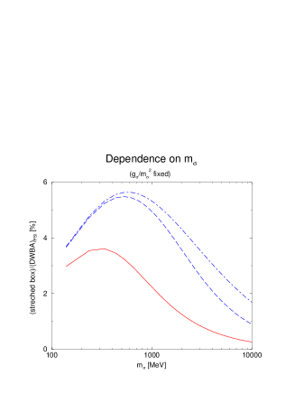
FIG. 2.: Importance of the stretched boxes for different choices of the cutoff as a function of the mass of the $\sigma$ meson. The ratios of the stretched boxes with respect to the DWBA piece, Eq. (11), are shown for $\Lambda=3m_{\pi}$ (solid line), $10m_{\pi}$ (dashed line) and $\infty$ (dot–dashed line).

The answer to the first question is obviously a function of the $\sigma$ mass, since the DWBA contributions should lead to results that are proportional to $(p_{i}/m_{\sigma})^{2}$, whereas the stretched boxes lead to $(p_{i}/m_{\sigma})^{4}$. In Fig. 2 we show the ratio of the stretched box contributions to the DWBA part as a function of the mass of the sigma meson. The three curves correspond to three different values of the cutoff for the radial integration. As expected, the curves all fall as $1/m_{\sigma}^{2}$ for large $m_{\sigma}$. The strength of the stretched boxes never exceeds 6%. This justifies a DWBA treatment of the final state in this pion production process.

The answer to the second question is presented in the left panel of Fig. 3 as a function of the cutoff in the momentum integration. We evaluated the DWBA piece, Eq. (11), with the exact propagator (13) and with the approximate propagator (15). The mass of the sigma was chosen to be $m_{\sigma}=550$ MeV. The solid curve shows the result using the approximate pion propagator in units of the exact result. Thus, the deviation of this approximation from the exact result never exceeds 25%.

FIG. 3.: Effects of the different approximations to the “production operator” for different cutoffs. The left (right) panel shows the result for a sigma exchange in the final (initial) state in units of the exact answer of Eq. (11) (Eq. (21)). Using the “fixed kinematics approximation” pion propagator leads to the solid curve. The dashed curve is the result when using the $(E-E^{\prime})$ approximation.

The third question goes to the choice of energy variable “$q_{0}$” at the $\pi N$ seagull vertex reported in the literature [4]. To simulate this choice we replace “$q_{0}$” = $m_{\pi}/2$ in the numerator of Eq.(11) with

$$``q_{0}"=E-E",$$ (16)

together with the approximate pion Klein-Gordon propagator. This was defined as the $(E-E^{\prime})$ prescription above. In many reactions Eq. (16) is an appropriate replacement, because the nucleons remain almost on the mass shell in the intermediate states. However, as soon as large intermediate momenta are accessible, this treatment might be questionable. In Fig. 3 the dashed curve shows the results of using the $(E-E^{\prime})$ prescription, again in units of the exact result. Within our toy model, the result shows that this approximation is not reasonable for calculations of threshold pion production. Note that this amplitude is very sensitive to the sigma mass, which acts as a regulator. If the sigma mass is taken to be larger, then the result changes even more dramatically with the cutoff. A change in sign happens at the point where the cutoff is big enough for the effect of the $\vec{k}^{2}/2M$ to overcome that of $m_{\pi}/2$ (the larger the intermediate momentum, the larger $E"$).

The net result of the toy model for the final-state interaction case is that using $``q_{0}"=m_{\pi}/2$ in both the virtual $\pi N$ seagull scattering vertex (numerator) and in the approximate pion Klein-Gordon propagator is very reasonable.

IV Initial–State Interaction

We now consider the case when the sigma exchange occurs before the re-scattering process. A reduction to the three-dimensional integral (or starting with the TOPT expression) gives the following four terms:

$$M_{I}=\int\frac{d^{3}q}{(2\pi)^{3}}\frac{\omega_{q}}{4\omega_{q}\omega_{\sigma}} \left\{\frac{2}{(E_{tot}-E^{\prime}-\bar{E}"-\omega_{q})(E_{tot}-2\bar{E}")(E_{tot}-E-\bar{E}"-\omega_{\sigma})}\right.$$ (20)

$$-\frac{2}{(E_{tot}-E^{\prime}-\bar{E}"-\omega_{q}-m_{\pi})(E_{tot}-2\bar{E}")(E_{tot}-E-\bar{E}"-\omega_{\sigma})}$$

$$+\frac{1}{(E_{tot}-E^{\prime}-\bar{E}"-\omega_{q})(E_{tot}-E-E^{\prime}-\omega_{q}-\omega_{\sigma})(E_{tot}-E-\bar{E}"-\omega_{\sigma})}$$

$$\left.-\frac{1}{(E_{tot}-E^{\prime}-\bar{E}"-\omega_{q}-m_{\pi})(E_{tot}-E-E^{\prime}-\omega_{q}-\omega_{\sigma}-m_{\pi})(E_{tot}-E-\bar{E}"-\omega_{\sigma})}\right\},$$

where again $\omega_{q}=\sqrt{m_{\pi}^{2}+\vec{q}\;^{2}}\;,\omega_{\sigma}=\sqrt{m_{\sigma}^{2}+(\vec{q}+\vec{p})^{2}}$, and $E^{\prime}=0$, but the energy of an intermediate nucleon is $\bar{E}"=\vec{q}\;^{2}/2M_{N}$.

As before, the first two terms in Eq. (20) correspond to box diagrams and the last two to stretched boxes, cf. Fig. 1. In case of the initial-state interaction the stretched boxes still turn out to be smaller than the boxes, but less so: $\simeq 30\%$. Note that this is also of the size expected in the real world where the expansion parameter of the EFT is $\sqrt{\frac{m_{\pi}}{M_{N}}}\simeq 0.4$ [2, 12]. We therefore concentrate on those terms containing the $NN$ propagator, $G_{NN}=(E_{tot}-2\bar{E}")^{-1}$, only and obtain

$$\int\frac{d^{3}q}{(2\pi)^{3}}\frac{m_{\pi}}{2}\;G_{\pi NN}^{TOPT}\left(\frac{1}{E_{tot}-2\bar{E}"}\right)V_{\sigma},$$ (21)

where

$$V_{\sigma}(\vec{q}\;^{2},\vec{k}\;^{2})=\frac{1}{\omega_{\sigma}(m_{\pi}/2-\bar{E}"-\omega_{\sigma})},$$ (22)

and in the initial-state interaction case the TOPT $\pi NN$ propagator reads

$$G_{\pi NN}^{TOPT}=\frac{1}{\left(\frac{m_{\pi}}{2}\right)^{2}-\left(\omega_{q}+\bar{E}"-\frac{m_{\pi}}{2}\right)^{2}}\ .$$ (23)

This looks like a DWBA expression using the $m_{\pi}/2$ prescription. Due to the large initial momentum, the unitarity cut of $G_{NN}$ turns out to be an essential feature.

Similar to the section on final-state interaction, we investigate the fixed kinematics approximation and the $E-E^{\prime}$ approximation using the free pionic Klein-Gordon propagator, Eq. (15). This means especially that in the $G_{\pi NN}^{TOPT}$ of Eq.(23) we set $\bar{E}"$ = $m_{\pi}/2$, which implies on-shell intermediate nucleons: $\vec{q}\,^{2}=m_{\pi}M_{N}$. In the $E-E^{\prime}$ approximation we further replace $``q_{0}"=m_{\pi}/2$ by $E-\bar{E}"$. In the right panel of Fig. 3 we demonstrate the inadequacy of both approximations, compared to the exact result given by Eq. (21).

Due to the large initial momentum the imaginary part of these diagrams turns out to be of the order of the real part. (Since we work at the kinematical threshold of pion production the imaginary part from $G_{\pi NN}$ is zero). Since all the approximations where constructed such that they agree once the intermediate two-nucleon state goes on-shell, all the individual results agree for the imaginary part.

The question becomes why do both approximations show such a large deviation from the exact result of Eq. (21). The cause can be traced back to the appearance of a $\pi NN$ cut in the exact propagator: from Eq. (23) we see that the propagator $G_{\pi NN}^{TOPT}$ diverges as $|\vec{q}|^{-2}$ when $\vec{q}$ approaches 0. On the other hand for small $\vec{q}$ the free pionic Klein-Gordon propagator $G_{\pi}^{KG}$ goes to a constant. It is the very different nature of the infrared behaviors of the propagators, $G_{\pi}^{KG}$ and $G_{\pi NN}^{TOPT}$, that leads to the large deviation of (the real part of) the amplitude from the result of Eq. (21).

Having identified the $\pi NN$ cut as an important feature of the production reaction, a natural question that arises is how to set up a counting scheme capable of covering this. Note that contrary to the more conventional contributions, where the scale of typical momenta is set by the initial momentum $p_{i}=\sqrt{M_{N}m_{\pi}}$, the $\pi NN$ cut pronounces momenta of the order of the external pion momentum. It can not be a part of a toy-model investigation to completely resolve this matter —after all our model interaction is not consistent with the requirements of chiral symmetry. However, we will use the last part of this section to suggest a possible method to address the issue.

To this end we will rewrite Eq. (20) such that we isolate both the $NN$ and the $\pi NN$ singularities. For this purpose we are guided by the unitarity transformation method of Ref. [16, 17]. This method is one way to isolate the different singularities of a particular diagram. In this case the scattering amplitude can be written as (where for clarity we suppress $\int d^{3}q$ as well as some over all factors) [18]:

$$M_{I} = M_{NN}+M_{\pi NN}+\cdots,$$ (24)

$$M_{NN} = \frac{1}{m_{\pi}-2\bar{E}"}\left(\frac{m_{\pi}/2}{\bar{E}"^{2}-\omega_{q}^{2}}\right)V_{\sigma},$$ (25)

$$M_{\pi NN} = -\frac{1}{m_{\pi}-\bar{E}"-\omega_{q}}\left(\frac{m_{\pi}/2}{\bar{E}"^{2}-\omega_{q}^{2}}\right)V_{\sigma},$$ (26)

where the ellipsis denote the stretched box TOPT diagram contributions. We see that the above amplitude has two physical singularities due to the $NN$ and $\pi NN$ scattering states. We find numerically that $M_{\pi NN}$ is about 5 times larger than $M_{NN}$ when evaluated with a cutoff of $\Lambda$ = 10$m_{\pi}$. This large effect of the $\pi NN$ cut in the toy model is also responsible for the stronger effect of initial-state stretched boxes, as the latter also contains the $\pi NN$ cut (see fourth line of Eq. (20)). These two points highlight the numerical significance of the three-particle cut.

Note that this is not a unique separation of the two branch cuts. To make closer contact with previous work [16, 17] we can rewrite Eq. (24) in a form closer to the $(E-E^{\prime})$ prescription:

$$M_{I} = M^{\prime}_{NN}+M^{\prime}_{\pi NN}+\cdots,$$ (27)

$$M^{\prime}_{NN} = \frac{1}{m_{\pi}-2\bar{E}"}\left(\frac{\bar{E}"}{\bar{E}"^{2}-\omega_{q}^{2}}\right)V_{\sigma},$$ (28)

$$M^{\prime}_{\pi NN} = -\frac{1}{m_{\pi}-\bar{E}"-\omega_{q}}\left(\frac{(\bar{E}"+\omega_{q})/2}{\bar{E}"^{2}-\omega_{q}^{2}}\right)V_{\sigma}.$$ (29)

Clearly $M_{NN}+M_{\pi NN}$ = $M_{NN}^{\prime}+M_{\pi NN}^{\prime}$, although some shift of strength is then achieved between $NN$ and $\pi NN$ contributions: in this case we find the contribution from $M_{\pi NN}^{\prime}$ larger in magnitude than $M_{NN}^{\prime}$ by a factor 2, using the same cutoff $\Lambda$ = 10$m_{\pi}$. It remains to be seen which splitting is the most appropriate in the realistic case.

The most significant finding for the case of the initial-state interaction is therefore that in the toy model the three-body $\pi NN$ branch cut of $G_{\pi NN}$ is very important. The importance of this cut has been advocated before, for example in Ref.[19]. Here the static propagator, which was defined as being part of the fixed kinematics approximation as well as of the $(E-E^{\prime})$ approximation, leads to erroneous results for the real part of the amplitude.

However, it is important to remark that we expect the importance of this branch cut to be much smaller in the real world. Indeed, as we have seen, close to threshold this type of contribution comes from three-momenta near 0. In the real world, chiral symmetry suppresses such contributions. The pion coupling in leading order in chiral perturbation theory, for example, goes through the pion three-momentum. In our toy, chiral symmetry does not play a role, the pion coupling is a simple Yukawa coupling, and both initial and final $NN$ states are in relative $S$ waves, which enhances the influence of the $\pi NN$ cut. The power counting developed in Refs. [2, 12] does take into account chiral symmetry —thus the correct factors of momenta— and suggests a suppression of these branch effects, as long as the momentum of the emitted pion is ${\cal O}(m_{\pi})$ (or less). Clearly, it is important to further study the power counting —in particular in conjunction with the unitary transformation method— in the realistic case.

V Summary and Conclusion

We have investigated various approximations for pion production by defining a toy model which allows the computation of exact model transition-matrix elements. Because it lacks chiral symmetry, this model has the unrealistic features that both the initial and final state $NN$ wave functions are $S$ states. The influence of $NN$ correlations that suppress the short-distance wave functions are absent from the toy model. Furthermore, diagrams with both initial- and final-state interactions could also be important in more realistic calculations. We have performed some test calculations using the Reid $NN$ potential, which indicate that $NN$ correlations do modify some of the toy model findings at a quantitative level. However, the toy model allows the compilation of exact results at a given order in the couplings, and thus some qualitative insight.

The findings of this paper can be summarized as follows:

• The stretched box contributions are numerically small compared with boxes.

• For the final-state interaction, only the fixed kinematics approximation (for both propagator and vertex) turns out to be appropriate.

• If a loop with the initial-state interaction is included, the contribution of the $\pi NN$ cut is very important and has to be taken into account properly, which is not done in the common approximations.

The first two findings are in accord with the expectation from the existing power counting for pion production in the effective field theory [2, 12]. Indeed, according to this power counting stretched boxes involving pions are sub-leading and those involving heavier mesons are absorbed in higher-order local operators. Moreover, due to infrared enhancements that lead to the (quasi) bound state in the $NN$ interaction, the effect of the final-state interaction in realistic calculations should be by far dominant close to threshold.

The third finding is perhaps surprising. However, chiral symmetry is expected to be crucial in suppressing this contribution in the real world, because the $\pi NN$ cut emphasizes small momenta. Clearly, the importance of the three-body nature of the intermediate state needs to be further examined in realistic calculations.

Acknowledgments: We would like to thank Harry Lee for hosting the INT/Argonne Workshop on Pion Production, where this work originated. For hospitality, FM and UvK thank the Nuclear Theory Group and the Institute for Nuclear Theory at the University of Washington, and TS thanks the Nuclear Theory Group at the University of South Carolina. CH would like to thank the Alexander von Humboldt Foundation for financial support. We thank the U.S. Department of Energy [grant DE-FG03-97ER41014 (GAM and UvK)] and the NSF [grants PHY-9900756 (FM) and PHY 94-20740 (UvK)] for partial support. UvK would also like to thank RIKEN, Brookhaven National Laboratory and the U.S. Department of Energy [grant DE-AC02-98CH10886] for providing the facilities essential for the completion of this work.

REFERENCES

- [1] H.O. Meyer et al., Phys. Rev. Lett. 65, 2846 (1990); Nucl. Phys. A539, 663 (1992).
- [2] T.D. Cohen, J.L. Friar, G.A. Miller, and U. van Kolck, Phys. Rev. C 53, 2661 (1996).
- [3] B.Y. Park et al., Phys. Rev. C 53, 1519 (1996).
- [4] T. Sato, T.-S.H. Lee, F. Myhrer, and K. Kubodera, Phys. Rev. C 56, 1246 (1997).
- [5] C. Hanhart et al., Phys. Lett. B424, 8 (1998).
- [6] U. van Kolck, G.A. Miller, and D.O. Riska, Phys. Lett. B388 679 (1996).
- [7] C.A. da Rocha, G.A. Miller, and U. van Kolck, Phys. Rev. C 61, 034613 (2000).
- [8] E. Gedalin, A. Moalem, and L. Razdolskaya, Phys. Rev. C 60, 31 (1999).
- [9] V. Dmitrasinovic, K. Kubodera, F. Myhrer, and T. Sato, Phys. Lett. B465, 43 (1999).
- [10] T.-S. Park, S. Ando, and D.-P. Min, nucl-th/0003004.
- [11] For an overview of recent developments, see C. Hanhart, STORI 99, Bloomington, Sept. 1999, U.W. preprint NT-UW-99-60, nucl-th/9911023.
- [12] C. Hanhart, G.A. Miller, and U. van Kolck, Phys. Rev. Lett. 85, 2905 (2000).
- [13] V. Bernard, N. Kaiser, and U.-G. Meißner, Nucl. Phys. B457, 147 (1995).
- [14] M.T. Peña, D.O. Riska, and A. Stadler, Phys. Rev. C 60 045201 (1999).
- [15] C. Hanhart et al., Phys. Lett. B358, 21 (1995).
- [16] N. Fukuda, K. Sawada, and M. Taketani, Prog. Theor. Phys. 12, 156 (1954); S. Okubo, Prog. Theor. Phys. 12, 603 (1954).
- [17] M. Kobayashi, T. Sato, and H. Ohtsubo, Prog. Theor. Phys. 98, 927 (1997).
- [18] Note, in the non-relativistic treatment the individual terms employ poles at . However, since this kinematic regime is beyond the applicability of the non-relativistic treatment anyhow and the cutoff is chosen to be well below this scale, we do not need to worry about these in the context of this presentation.
- [19] B. Blankleider, AIP Conf. Proc. 221, Particle and Fields Series 41, “Particle Production near Threshold”, eds. H. Nann and E.J. Stephenson, (1991) p.150; see also later publications found in A.N. Kvinikhidze and B. Blankleider, Phys. Rev. C 59, 1263 (1999).