Field Redefinitions at Finite Density

Abstract

The apparent dependence of nuclear matter observables on off-shell properties of the two-nucleon potential is re-examined in the context of effective field theory (EFT). Finite density (thermodynamic) observables are invariant under field redefinitions, which extends the well-known theorem about the invariance of S-matrix elements. Simple examples demonstrate how field redefinitions can shift contributions between purely off-shell two-body interactions and many-body forces, leaving both scattering and finite-density observables unchanged. If only the transformed two-body potentials are kept, however, the nuclear matter binding curves will depend on the off-shell part (generating “Coester bands”). The correspondence between field redefinitions and unitary transformations, which have traditionally been used to generate “phase-equivalent” nucleon-nucleon potentials, is also demonstrated.

I Introduction

Over thirty years ago, it was observed that “phase-equivalent” nucleon-nucleon potentials gave different predictions when used to calculate the energy per particle of nuclear matter [1, 2, 3, 4]. Phase equivalent means that the potentials predict identical two-nucleon observables (phase shifts and binding energies); families of such potentials can be constructed via unitary transformations [5]. The finite-density discrepancies were attributed to the differing off-shell behavior of the nucleon-nucleon (NN) amplitude or T-matrix, and were related semi-quantitatively to the distortion of the two-body relative wave function in the medium (the “wound integral”) [1]. It was proposed that comparisons of nuclear matter calculations could help to determine the correct off-shell dependence [4, 6].

From the modern perspective of effective field theory (EFT), these results demand a different interpretation, since off-shell effects are not observable. Phase-equivalent EFT potentials should give the same result for all observables (up to expected truncation errors) if consistent power counting is used; differences imply that something is missing. In this paper, we show how this issue is resolved by considering field redefinitions at finite density in an effective field theory.

There is an extensive literature, primarily from the sixties and seventies, on the role of off-shell physics in nuclear phenomena (see, e.g., Ref. [6] and references therein). This includes not only few-body systems (e.g., the triton) and nuclear matter, but interactions of two-body systems with external probes, such as nucleon-nucleon bremstrahlung and the electromagnetic form factors of the deuteron. The implicit premise, which persists today, is that there is a true underlying potential governing the nucleon-nucleon force, so that its off-shell properties can be determined. Indeed, the nuclear many-body problem has traditionally been posed as finding approximate solutions to the many-particle Schrödinger equation, given a fundamental two-body interaction that reproduces two-nucleon observables.

An alternative approach to nuclear phenomena is that of effective field theory. The EFT approach exploits the separation of scales in physical systems [7, 8, 9, 10, 11, 12, 13]. Only low-energy (or long-range) degrees of freedom are included explicitly, with the rest parametrized in terms of the most general local (contact) interactions. Using renormalization, the influence of high-energy states on low-energy observables is captured in a small number of constants. Thus, the EFT describes universal low-energy physics independent of detailed assumptions about the high-energy dynamics. The application of EFT methods to many-body problems promises a consistent organization of many-body corrections, with reliable error estimates, and insight into the analytic structure of observables. EFT provides a model independent description of finite density observables in terms of parameters that can be fixed from scattering in the vacuum.

A fundamental theorem of quantum field theory states that physical observables (or more precisely, S-matrix elements) are independent of the choice of interpolating fields that appear in a Lagrangian [14, 15]. Equivalently, observables are invariant under a change of field variables in a field theory Lagrangian (or Hamiltonian). This “equivalence theorem” holds for renormalized field theories, although there are subtleties with some regularizations [16]. In an EFT, one exploits the invariance under field redefinitions to eliminate redundant terms in the effective Lagrangian and to choose the most convenient or efficient form for practical calculations [17, 18, 19, 20, 21, 22]. Since off-shell Green’s functions and the corresponding off-shell amplitudes do change under field redefinitions, one must conclude that off-shell properties are unobservable.

Several recent works have emphasized from a field theory point of view the impossibility of observing off-shell effects. In Refs. [23, 24], model calculations are used to illustrate how apparent determinations of the two-nucleon off-shell T-matrix in nucleon-nucleon bremstrahlung are illusory, since field redefinitions shift contributions between off-shell contributions and contact interactions (see Sec. III). Similarly, it was shown in Ref. [25] that Compton scattering on a pion cannot be used to extract information on the off-shell behavior of the pion form factor. The authors of Refs. [26, 27] emphasized the nonuniqueness of chiral Lagrangians for three-nucleon forces and pion production. Field redefinitions lead to different off-shell forms that yield the same observables within a consistent power counting. In Ref. [28], an interaction proportional to the equation of motion is shown to have no observable consequence for the deuteron electromagnetic form factor, even though it contributes to the off-shell T-matrix.

In systems with more than two nucleons, one can trade off-shell, two-body interactions for many-body forces. This explains how two-body interactions related by unitary transformations can predict different binding energies for the triton [29] if many-body forces are not consistently included. These issues are discussed from the viewpoint of unitary transformations in Refs. [30] and [31]. An EFT analysis of the triton with short-range forces was performed by Bedaque and collaborators. They showed that a three-body counterterm is needed in the triton for consistency [32]. Varying this counterterm generates a one-parameter family of observables, which explains the Phillips line.

Here we consider fermion systems in the thermodynamic limit. We extend the equivalence theorem to finite density observables, or thermodynamic observables in general, and show the consequence of field redefinitions. Since the thermodynamic observables are conveniently expressed in a functional integral formalism, we adapt the discussion in Ref. [21], which provides a particularly transparent (if not entirely rigorous) account of the equivalence theorem for S-matrix elements and how it can be applied in EFT’s, based on functional integrals. We show how field redefinitions applied to an EFT Lagrangian with only on-shell vertices generate new off-shell vertices, which by themselves change predictions for an infinite system. However, many-body vertices are also induced, and if included consistently, will precisely cancel the off-shell parts. In the end, all calculations agree, with no off-shell ambiguities.

In section II, we review the argument in Ref. [21], extend it to thermodynamic observables, and show how field redefinitions can reduce an effective Lagrangian to a canonical form. In section III, we illustrate the effects of field redefinitions with a simple example applied to the dilute Fermi gas of Ref. [33]. The connection to traditional treatments is elucidated in section IV. Finally, we summarize in Section V.

II Field Redefinitions

The equivalence theorem is typically stated as the invariance of the S-matrix for asymptotic scattering states under a change of field variables. Intuitive diagrammatic proofs, as in Refs. [34, 35], are based on the reduction formula for calculating S-matrix elements from on-shell Green’s functions. The proofs show that field redefinitions change only the wave function renormalization, which is divided out in the reduction formula. The extension to observables in the thermodynamic limit, such as the energy density of an infinite system of fermions at zero temperature, is not obvious since there are no asymptotic single-particle states. Here we make that extension for nonrelativistic systems and discuss the consequences for effective field theories. The generalization to covariant effective field theories is straightforward.

A rigorous proof of the equivalence theorem must include a careful discussion of renormalized Green’s functions and amplitudes, and the impact of different regulators. Such a proof, based on the renormalized quantum action principles, is given in Ref. [16] and extended to a heavy-fermion expansion (in the context of heavy quark effective field theory) in Ref. [19]. The new issues in considering thermodynamic observables, however, do not change the subtle technical issues in the proof, so we build instead on a less rigorous but more intuitive path integral discussion of the equivalence theorem [21] to illustrate the broad concepts and consequences. The path-integral formalism is convenient, since one can generate Green’s functions and subsequently S-matrix elements, as well as thermodynamic observables, in the same framework.

We will only consider heavy (nonrelativistic) boson or fermion fields explicitly; the generalization to include long-range bosonic fields (e.g., such as the pion) is straightforward. The procedure that leads from an underlying relativistic theory to an effective Lagrangian ${\cal L}$ in a heavy-particle formulation is outlined in Ref. [12]. We work in the rest frame, so there are no non-trivial four-velocities associated with the field variables. In general, ${\cal L}$ contains all terms consistent with the usual space-time symmetries as well as any symmetries of the underlying theory. These include, in general, higher-order time derivatives, which can be eliminated as described below. The path integral form of the generating functional is written schematically as:

$$Z[\xi^{\dagger},\xi]=\int\!{\cal D}(\psi^{\dagger},\psi)\,e^{i\int{\cal L}[\psi,\psi^{\dagger}]+\xi^{\dagger}\psi+\psi^{\dagger}\xi}\ ,$$ (1)

where $\psi$ and $\psi^{\dagger}$ are Grassmann variables for fermions, $\xi^{\dagger}$ and $\xi$ are external Grassmann sources. By taking functional derivatives of $Z$ with respect to the sources, we generate the $n$-body Green’s functions and then S-matrix elements via a reduction formula.

Here we follow the discussion of the equivalence theorem in Ref. [21]. The basic observation is that if we change field variables in the functional integral, predictions for given external sources should be unchanged. Consider a transformation of $\psi$ of the form:

$$\psi(x)\longrightarrow\psi(x)+\eta T[\psi,\psi^{\dagger}]\ ,$$ (2)

where $T[\psi,\psi^{\dagger}]$ is a local polynomial in $\psi(x)$, $\psi^{\dagger}(x)$, and their derivatives, and $\eta$ is an arbitrary counting parameter (to be used below). The transformation given by Eq. (2) is local and respects the symmetries of ${\cal L}$. There are no space-time dependent external parameters, i.e. the $x$-dependence of $T[\psi,\psi^{\dagger}]$ comes from the fields alone. Specific examples of such transformations are given in Eqs. (21) and (74).

Within the path integral, three types of change result from Eq. (2):

1. the Lagrangian changes: ${\cal L}\rightarrow{\cal L}^{\prime}$;

2. there is a Jacobian from the transformation;

3. there are additional terms coupled to the external sources $\xi$ and $\xi^{\dagger}$.

The statement of the equivalence theorem is that changes 2 and 3 by themselves do not affect observables, so that one is free to change variables in the Lagrangian alone. By introducing ghost fields, the Jacobian from 2 can be exponentiated. As detailed in Ref. [21], new terms involving ghosts either decouple or contribute pure power divergences in ghost loops. The latter are either zero in dimensional regularization or can be absorbed without physical consequence into couplings in ${\cal L}$. Therefore the Jacobian has no observable effect. The extra terms in 3 do change the Green’s functions but not the S-matrix. The proof is analogous to the usual diagrammatic proof [21].

To extend the discussion to finite density and/or temperature, we consider a Euclidean path integral formulation of the partition function $Z$ and thermodynamic potential $\Omega$:

$$Z\equiv\exp(-\beta\Omega)\equiv{\rm Tr}\{\exp[-\beta(\widehat{H}-\mu\widehat{N})]\}\ ,$$ (3)

where $\beta$ is the inverse temperature, $\mu$ is the chemical potential, $\widehat{H}$ is the Hamiltonian, and $\widehat{N}$ is the number operator (e.g., the baryon number for nuclear systems). The hat indicates second quantized operators that act in Fock space. We direct the reader to Ref. [37] for details on the derivation and interpretation of nonrelativistic path integrals at finite temperature and chemical potential. The connection between $\widehat{H}$ and ${\cal L}$ is complicated, but we do not need to actually derive the connection, since we assume a general form for ${\cal L}$. However, we need to be more explicit with $\widehat{N}$, which is not in general equal to the spatial integral of $\psi^{\dagger}\psi$. Instead, the appropriate operator should be derived using Noether’s theorem applied to ${\cal L}$.

The integrations in the path integral corresponding to Eq. (3) will be over complex variables satisfying periodic boundary conditions in imaginary time for bosons and over Grassmann variables satisfying antiperiodic boundary conditions for fermions. If there is no chemical potential, the extension of the equivalence theorem to finite temperature is immediate, because the finite temperature boundary conditions are trivially preserved by field redefinitions of the form in Eq. (2) and the remainder of the argument is unchanged. Thus the thermodynamic quantities derived from the partition function (e.g., free energies and specific heats) will be invariant under field redefinitions for all $\beta$. Since there are no external sources, we are free to introduce linearly coupled sources to construct a perturbative expansion after the field redefinitions.

A nonzero chemical potential will be multiplied by new terms after the field redefinition. The conserved current is associated with a global $U(1)$ symmetry transformation

$$\psi(x)\longrightarrow e^{-i\phi}\psi(x)\quad\mbox{ and }\quad{\psi^{\dagger}}(x)\longrightarrow e^{i\phi}{\psi^{\dagger}}(x)\ ,$$ (4)

under which ${\cal L}$ is invariant. We can conveniently identify the Noether current by promoting $\phi$ to a function of $x$ and considering infinitesimal transformations with [36]

$${\cal L}\longrightarrow\widetilde{\cal L}[\psi,\psi^{\dagger};\phi(x)]\ .$$ (5)

Then the charge density $\widehat{\rho}$ is given by

$$\widehat{\rho}\equiv\frac{\delta}{\delta(\partial_{t}\phi)}\widetilde{\cal L}[\psi,\psi^{\dagger};\phi(x)]\equiv F[\psi,\psi^{\dagger}]\ .$$ (6)

The possibility of higher-order time derivatives or time derivatives in non-quadratic terms in $\widetilde{\cal L}$ means that, in general, $F[\psi,\psi^{\dagger}]\neq\psi^{\dagger}\psi$.

Under the transformation Eq. (2),

$${\cal L}[\psi,\psi^{\dagger}]\longrightarrow{\cal L}^{\prime}[\psi,\psi^{\dagger}] = {\cal L}[\psi+\eta T,\psi^{\dagger}+\eta T^{\dagger}]$$ (7)

$$= {\cal L}+\Bigl{(}\eta T\frac{\delta{\cal L}}{\delta\psi}+\mbox{H.c.}\Bigr{)}+\cdots\ ,$$ (8)

while

$$F[\psi,\psi^{\dagger}]\longrightarrow F^{\prime}[\psi,\psi^{\dagger}] = F[\psi+\eta T,\psi^{\dagger}+\eta T^{\dagger}]$$ (9)

$$= F+\Bigl{(}\eta T\frac{\delta F}{\delta\psi}+\mbox{H.c.}\Bigr{)}+\cdots\ ,$$ (10)

where we have written the first terms in the functional Taylor expansions of Eqs. (8, 10) and H.c. denotes the Hermitian conjugate. If $T$ contains no time derivatives (as in the examples in Sections III and IV), then using the fact that $\delta/\delta(\partial_{t}\phi)$ commutes with $\delta/\delta\psi$, we see order-by-order in $\eta$ that

$${\widehat{\rho}}\,^{\prime}\equiv\frac{\delta}{\delta(\partial_{t}\phi)}\widetilde{\cal L}^{\prime}[\psi,\psi^{\dagger};\phi(x)]=F^{\prime}[\psi,\psi^{\dagger}]\ .$$ (11)

So the term multiplying $\mu$ in the transformed path integral is the new charge density. If $T$ contains time derivatives, ${\widehat{\rho}}\,^{\prime}$ will contain additional terms proportional to the equations of motion, which give zero contribution [19, 21].

At zero temperature, we can work without an explicit chemical potential, but instead specify the density through boundary conditions in the noninteracting propagator (see Sect. III). Using the new charge density operator, we find the density is unchanged by the transformation. This is illustrated explicitly for a special case in the Appendix.

For an effective field theory, invariance under nonlinear field redefinitions has practical and philosophical implications. On the practical side, because the EFT already contains all terms consistent with the underlying symmetries (which are preserved by the field variable changes we consider), there is no penalty for making such transformations: they just change the coefficients of existing terms. Therefore, we can use this freedom to remove redundant terms and define a canonical form of the EFT Lagrangian. This can simplify the calculation or improve its convergence. One possibility is what Georgi calls “on-shell effective field theory,” which features only those vertices that are non-zero for on-shell kinematics (of free particles) [18]. This was the choice in Ref. [33], which treated dilute Fermi systems.

An effective Lagrangian is organized according to a hierarchy, which we label by $\eta$ [21]:

$${\cal L}=\sum_{n=0}^{\infty}\eta^{n}{\cal L}_{n}\ .$$ (12)

For example, we have $\eta\propto 1/\Lambda$ for a natural field theory as in Ref. [33]. Define ${\cal L}_{0}$ to be:

$${\cal L}_{0}=\psi^{\dagger}\biggl{[}i\partial_{t}+\frac{\overrightarrow{\nabla}^{2}\!}{2M}\biggr{]}\psi\ .$$ (13)

As a result of the transformation Eq. (2), ${\cal L}\rightarrow{\cal L}^{\prime}$, with

$${\cal L}^{\prime}={\cal L}_{0}+\biggl{(}\eta T[\psi,\psi^{\dagger}]\biggl{[}i\partial_{t}+\frac{\overrightarrow{\nabla}^{2}\!}{2M}\biggr{]}\psi+\mbox{H.c.}\biggr{)}+\sum_{n=1}^{\infty}\eta^{n}{\cal L}^{\prime}_{n}\ .$$ (14)

Thus, at leading order in $\eta$, we generate a term proportional to the free equation of motion. The corresponding interaction term will be proportional to the inverse free propagator, and thus will vanish on shell. So we can change off-shell Green’s functions (e.g., the two-nucleon off-shell T-matrix) by field transformations without changing observables. The consequence is that one can change the appearance of ${\cal L}$. One may find that better convergence of an EFT expansion is correlated with a particular off-shell dependence, but the idea of measuring the “correct” off-shell behavior has to be dismissed. These implications are extended to conventional approaches to nuclear phenomena by considering them as implementations, albeit incomplete, of the EFT approach. The discussion can be directly extended to a finite system with a single particle potential included in ${\cal L}_{0}$ (and in the noninteracting propagator).

We are also able to remove redundant terms, which was implicit in the choice of the “general” effective Lagrangian in Ref. [33]. Time derivatives other than the quadratic term can be systematically eliminated by field redefinitions of the form in Eq. (2) by exploiting the EFT hierarchy. In particular, the lower-order (in $\eta$) terms can be removed at the cost of changing the coefficients of higher-order terms in $\eta$. For example, suppose we have the Lagrangian

$${\cal L}=\psi^{\dagger}\biggl{[}i\partial_{t}+\frac{\overrightarrow{\nabla}^{2}\!}{2M}\biggr{]}\psi+\eta_{1}\psi^{\dagger}(i\partial_{t})^{2}\psi+\eta_{2}\bigg{(}\psi^{\dagger}\frac{\tensor{\nabla}^{2}}{2M}(i\partial_{t})\psi+\mbox{ H.c.}\bigg{)}+{\cal O}(\eta^{2})\ ,$$ (15)

where $\tensor{\nabla}=\overleftarrow{\nabla}-\overrightarrow{\nabla}$. The field redefinition

$$\psi \longrightarrow \psi-\frac{\eta_{1}}{2}(i\partial_{t}\psi)+\Bigl{(}\frac{\eta_{1}}{2}-4\eta_{2}\Bigr{)}\frac{\overrightarrow{\nabla}^{2}\!}{2M}\psi\ ,$$ (16)

$${\psi^{\dagger}} \longrightarrow {\psi^{\dagger}}+\frac{\eta_{1}}{2}(i\partial_{t}{\psi^{\dagger}})+\Bigl{(}\frac{\eta_{1}}{2}-4\eta_{2}\Bigr{)}\frac{\overrightarrow{\nabla}^{2}\!}{2M}{\psi^{\dagger}}\ ,$$ (17)

results in the new Lagrangian

$${\cal L}^{\prime}=\psi^{\dagger}\biggl{[}i\partial_{t}+\frac{\overrightarrow{\nabla}^{2}\!}{2M}\biggr{]}\psi+\Bigl{(}\eta_{1}-8\eta_{2}\Bigr{)}\psi^{\dagger}\Bigl{(}\frac{\overrightarrow{\nabla}^{2}\!}{2M}\Bigr{)}^{2}\psi+{\cal O}(\eta^{2})\ ,$$ (18)

with no time derivatives outside of ${\cal L}_{0}$ to order $\eta$. Once we remove terms up to some order in $\eta$, further transformations will not reintroduce them because they involve the next higher order.

Equation (14) shows that different choices of effective Lagrangians, related by field redefinitions, can differ by off-shell contributions. The equivalence theorem guarantees that these must ultimately be canceled in observables (or vanish individually). In a sense, that makes any explicit demonstration “trivial”. The realization of the equivalence theorem, however, is often counterintuitive. Approximations in a truncated theory have to be consistent with this realization. A common source of confusion arises in discussions that assume only two-body vertices are kept in many-body calculations. Therefore, we turn to some concrete examples.

III Perturbative Examples

A Transformation of the Lagrangian

In this section, we illustrate the connection between off-shell two-body terms and three-body terms using a simple field redefinition. In particular, the effect of an off-shell vertex generated by a field redefinition is exactly canceled by a three-body term generated by the same transformation. We demonstrate this cancellation explicitly for the process of $3\to 3$ scattering in the vacuum and for the energy density of a dilute Fermi system at finite density. For simplicity, we consider a natural EFT for heavy nonrelativistic fermions of mass $M$ that has spin independent $s$-wave interactions whose strength is correctly estimated by naive dimensional analysis. Such a theory is discussed in detail, e.g., in Refs. [33, 39].

For a natural theory all effective range parameters are of order $1/\Lambda$, where $\Lambda$ is the breakdown scale of the theory. For momenta $k\ll\Lambda$, all interactions appear short-ranged and can be modeled by contact terms. We consider a local Lagrangian for a nonrelativistic fermion field that is invariant under Galilean, parity, and time-reversal transformations:

$${\cal L} = \psi^{\dagger}\biggl{[}i\partial_{t}+\frac{\overrightarrow{\nabla}^{2}\!}{2M}\biggr{]}\psi-\frac{C_{0}}{2}(\psi^{\dagger}\psi)^{2}+\frac{C_{2}}{16}\Bigl{[}(\psi\psi)^{\dagger}(\psi\tensor{\nabla}^{2}\psi)+\mbox{ H.c.}\Bigr{]}+\ldots\,,$$ (19)

where $\tensor{\nabla}=\overleftarrow{\nabla}-\overrightarrow{\nabla}$ is the Galilean invariant derivative and H.c. denotes the Hermitian conjugate. Higher-order time derivatives are not included, since it is most convenient for our purposes to eliminate them in favor of gradients, as described in Sec. II. Naive dimensional analysis estimates $C_{2i}$ to be roughly $4\pi/(M\Lambda^{2i+1})$, which implies a perturbative expansion in $k/\Lambda$. $C_{0}$ and $C_{2}$ can be related to the $s$-wave scattering length $a$ and effective range $r_{e}$ via a matching calculation. This leads to the relations

$$C_{0}=\frac{4\pi a}{M}\quad\mbox{and}\quad C_{2}=C_{0}\frac{ar_{e}}{2}\,.$$ (20)

We stress that we choose this simple example to make the cancellation of off-shell effects in observables as transparent as possible. As follows from the general discussion in the previous section, analogous cancellations occur in more complicated theories that include long-range physics, relativistic effects, spin-dependent interactions, nonperturbative resummations and so on.

We generate a new Lagrangian ${\cal L}^{\prime}$ by performing the field transformation

$$\psi \to \psi+\frac{4\pi\alpha}{\Lambda^{3}}(\psi^{\dagger}\psi)\psi\,,\qquad\psi^{\dagger}\to\psi^{\dagger}+\frac{4\pi\alpha}{\Lambda^{3}}\psi^{\dagger}(\psi^{\dagger}\psi)\,,$$ (21)

on ${\cal L}$. The factor $1/\Lambda^{3}$ is introduced to keep the arbitrary parameter $\alpha$ dimensionless. The additional factor of $4\pi$ is introduced for convenience. With this choice, the induced terms have the size expected from naive dimensional analysis if $\alpha$ is of order unity. We obtain for ${\cal L}^{\prime}$:

$${\cal L}^{\prime} = {\cal L}-\frac{4\pi\alpha}{\Lambda^{3}}2C_{0}({\psi^{\dagger}}\psi)^{3}$$ (22)

$$+ \frac{4\pi\alpha}{\Lambda^{3}}\frac{C_{2}}{8}\left\{2({\psi^{\dagger}}\psi)(\psi\psi)^{\dagger}(\psi\tensor{\nabla}^{2}\psi)+({\psi^{\dagger}}\psi)^{2}\left[(\overrightarrow{\nabla}^{2}\!{\psi^{\dagger}})\psi+{\psi^{\dagger}}(\overrightarrow{\nabla}^{2}\!\psi)+2(\overrightarrow{\nabla}{\psi^{\dagger}})(\overrightarrow{\nabla}\psi)\right]+\mbox{ H.c.}\right\}$$ (23)

$$+ \frac{4\pi\alpha}{\Lambda^{3}}\left\{({\psi^{\dagger}}\psi){\psi^{\dagger}}({i\partial_{t}}\psi)-\frac{1}{2M}\left[{\psi^{\dagger}}(\overrightarrow{\nabla}\psi)\cdot{\psi^{\dagger}}(\overrightarrow{\nabla}\psi)+2(\overrightarrow{\nabla}{\psi^{\dagger}})\psi\cdot{\psi^{\dagger}}(\overrightarrow{\nabla}\psi)\right]+\mbox{ H.c.}\right\}$$ (24)

$$+ \mbox{ 4- and higher-body terms }+{\cal O}(\alpha^{2})\,,$$ (25)

where 4- and higher-body terms as well as terms of ${\cal O}(\alpha^{2})$ have been omitted.

The two-body vertices generated by the transformed Lagrangian ${\cal L}^{\prime}$ are shown in Fig. 1.

FIG. 1.: Two-body vertices generated by ${\cal L}^{\prime}$. The corresponding Feynman rules are given in Eq. (28).

The vertices (i) and (ii) were already present in the untransformed Lagrangian ${\cal L}$, while (iii) is a new energy-dependent off-shell vertex of ${\cal O}(\alpha)$, which vanishes identically if all lines are on-shell. However, ${\cal L}^{\prime}$ also contains two new three-body vertices of ${\cal O}(\alpha C_{0})$ and ${\cal O}(\alpha C_{2})$. These vertices are illustrated in Fig. 2. The spin projection of a particle with energy $\omega_{i}(\omega^{\prime}_{j})$ and momentum ${\bf p}_{i}({\bf p^{\prime}}_{j})$ is denoted by $s^{\vphantom{x}}_{i}(s^{\prime}_{j})$; we abbreviate $\delta_{s^{\vphantom{x}}_{i}s^{\prime}_{j}}\equiv\delta_{ij^{\prime}}$. Note that $\omega_{i}\not={\bf p}_{i}^{2}/(2M)$ unless the particle is on shell. The Feynman rules for all vertices are listed below.

FIG. 2.: Three-body vertices generated by ${\cal L}^{\prime}$. The corresponding Feynman rules are given in Eq. (32).

• Two-body vertices:

  (i) $$-iC_{0}\,S_{2}$$ (26)

  (ii) $$-i\frac{C_{2}}{8}\left\{({\bf p}_{1}-{\bf p}_{2})^{2}+({\bf p^{\prime}}_{1}-{\bf p^{\prime}}_{2})^{2}\right\}S_{2}$$ (27)

  (iii) $$i\frac{4\pi\alpha}{\Lambda^{3}}\left\{\omega_{1}+\omega_{2}+\omega^{\prime}_{1}+\omega^{\prime}_{2}-\frac{1}{2M}\left[{\bf p}_{1}^{2}+{\bf p}_{2}^{2}+{\bf p^{\prime}}_{1}^{2}+{\bf p^{\prime}}_{2}^{2}\right]\right\}S_{2}$$ (28)

• Three-body vertices:

  (iv) $$-i\frac{4\pi\alpha}{\Lambda^{3}}12C_{0}\,S_{3}$$ (29)

  (v) $$-i\frac{4\pi\alpha}{\Lambda^{3}}\frac{C_{2}}{2}\sum_{{\rm Perm}\{1^{\prime},2^{\prime},3^{\prime}\}}\delta_{11^{\prime}}\delta_{22^{\prime}}\delta_{33^{\prime}}\;\epsilon_{1^{\prime}2^{\prime}3^{\prime}}\left[({\bf p}_{1}-{\bf p}_{2})^{2}\right.$$ (30)

  $$\ \left.+({\bf p}_{1}-{\bf p}_{3})^{2}+({\bf p}_{1}-{\bf p^{\prime}}_{1})^{2}+({\bf p}_{2}-{\bf p}_{3})^{2}+({\bf p}_{2}-{\bf p^{\prime}}_{2})^{2}\right.$$ (31)

  $$\ \left.+({\bf p}_{3}-{\bf p^{\prime}}_{3})^{2}+({\bf p^{\prime}}_{1}-{\bf p^{\prime}}_{2})^{2}+({\bf p^{\prime}}_{1}-{\bf p^{\prime}}_{3})^{2}+({\bf p^{\prime}}_{2}-{\bf p^{\prime}}_{3})^{2}\right]$$ (32)

The sum in (v) runs over all permutations of $\{1^{\prime},2^{\prime},3^{\prime}\}$ and $\epsilon_{ijk}$ is the totally antisymmetric Levi-Civita tensor with $\epsilon_{1^{\prime}2^{\prime}3^{\prime}}=-\epsilon_{2^{\prime}1^{\prime}3^{\prime}}=1$. Note that vertex (v) can be rewritten in terms of the total momentum ${\bf P}={\bf p}_{1}+{\bf p}_{2}+{\bf p}_{3}$ as

(v) $$-i\frac{4\pi\alpha}{\Lambda^{3}}C_{2}\sum_{{\rm Perm}\{1^{\prime},2^{\prime},3^{\prime}\}}\delta_{11^{\prime}}\delta_{22^{\prime}}\delta_{33^{\prime}}\;\epsilon_{1^{\prime}2^{\prime}3^{\prime}}\left[3{\bf P}^{2}-{\bf p}_{1}\cdot{\bf p^{\prime}}_{1}-{\bf p}_{2}\cdot{\bf p^{\prime}}_{2}-{\bf p}_{3}\cdot{\bf p^{\prime}}_{3}\right]\ .$$ (33)

The spin functions $S_{2}$ and $S_{3}$ are given by

$$S_{2} = {\delta_{11^{\prime}}\delta_{22^{\prime}}-\delta_{12^{\prime}}\delta_{21^{\prime}}}\ ,$$ (34)

$$S_{3} = {\delta_{11^{\prime}}(\delta_{22^{\prime}}\delta_{33^{\prime}}-\delta_{23^{\prime}}\delta_{32^{\prime}})+\delta_{12^{\prime}}(\delta_{23^{\prime}}\delta_{31^{\prime}}-\delta_{21^{\prime}}\delta_{33^{\prime}})+\delta_{13^{\prime}}(\delta_{21^{\prime}}\delta_{32^{\prime}}-\delta_{22^{\prime}}\delta_{31^{\prime}})}\ ,$$ (35)

for spin-1/2 fermions and by $S_{2}=2$ and $S_{3}=6$ for spin-0 bosons. The propagator for a particle line with energy $\omega$ and momentum ${\bf q}$ is simply

$$iS_{0}(\omega,{\bf q})=\frac{i}{\omega-{\bf q}^{2}/(2M)+i\epsilon}\ .$$ (36)

As discussed in Sec. II, the Lagrangian ${\cal L}^{\prime}$ has to give the same results for observables as the original Lagrangian ${\cal L}$. For this to happen, certain combinations of diagrams involving vertices (iii), (iv), and (v) have to cancel. As $\alpha$, $C_{0}$, and $C_{2}$ are independent parameters, this has to occur at every order in $\alpha$, $C_{0}$, and $C_{2}$ independently. In the following two subsections, we illustrate this cancellation for $3\to 3$ scattering in the vacuum and for the energy density at finite density.

B Cancellations at Zero Density

As mentioned above, all diagrams within one order of $\alpha$ have to cancel identically. Furthermore, the power counting of the original, untransformed theory carries over. The simplest example is the tree-level $2\to 2$ diagram with vertex (iii) which vanishes identically when all external legs are on shell so that the cancellation at ${\cal O}(\alpha)$ is trivial. Similarly, it is straightforward to show that all diagrams at ${\cal O}(\alpha C_{0}^{k}C_{2}^{l})$ that are bubble chains including $k$ vertices of type (i) and $l$ vertices of type (ii) plus one vertex of type (iii) vanish as well. This is most easily seen in dimensional regularization, where all vertices are on shell.

In the following, we consider $3\to 3$ scattering, where cancellations between different diagrams occur. We concentrate on the case of spin-1/2 fermions. The case of spin-0 bosons is analogous but somewhat simpler, because the spin function is trivial. At ${\cal O}(\alpha C_{0})$, we have the three tree-diagrams shown in Fig. 3. The external lines are labeled as in Fig. 2.

FIG. 3.: Additional diagrams for $3\to 3$ scattering generated by ${\cal L}^{\prime}$ at ${\cal O}(\alpha C_{0})$. The external lines are labeled as in Fig. 2.

Using the Feynman rules from Eqs. (28)–(36), we find for diagram 3(a),

$${{\cal M}}_{\rm\ref{alphaC0}(a)} = i\frac{4\pi\alpha}{\Lambda^{3}}C_{0}\left(\delta_{11^{\prime}}\delta_{22^{\prime}}\delta_{33^{\prime}}-\delta_{11^{\prime}}\delta_{23^{\prime}}\delta_{32^{\prime}}-\delta_{12^{\prime}}\delta_{21^{\prime}}\delta_{33^{\prime}}+\delta_{13^{\prime}}\delta_{21^{\prime}}\delta_{32^{\prime}}\right)\,,$$ (37)

where the internal propagator was canceled against the corresponding dependence of the off-shell vertex. At this point, we have to take into account that the cyclic permutations of the incoming and outgoing lines in diagram 3(a) generate topologically distinct diagrams that have to be included as well. Consequently, diagram 3(a) really represents nine diagrams, which when taken together generate the full spin function $S_{3}$. After summing over the cyclic permutations of the incoming and outgoing lines, we obtain

$${\cal M}_{\rm\ref{alphaC0}(a)}=6i\frac{4\pi\alpha}{\Lambda^{3}}C_{0}S_{3}={\cal M}_{\rm\ref{alphaC0}(b)}\,.$$ (38)

Evaluating diagram 3(b) gives exactly the same result as diagram 3(a). Finally, diagram 3(c) is simply given by vertex (iv). Adding the contribution of all diagrams at ${\cal O}(\alpha C_{0})$ we find

$${\cal M}_{\rm\ref{alphaC0}(a)}+{\cal M}_{\rm\ref{alphaC0}(b)}+{\cal M}_{\rm\ref{alphaC0}(c)}=0\ ,$$ (39)

and to ${\cal O}(\alpha C_{0})$ the off-shell dependence introduced by vertex (iii) cancels identically. A similar cancellation occurs for the diagrams at ${\cal O}(\alpha C_{2})$ where the $C_{0}$ vertex in Fig. 3 is replaced by a $C_{2}$ vertex and vertex (iv) is replaced by vertex (v). The corresponding diagrams are shown in Fig. 4.

FIG. 4.: Additional diagrams for $3\to 3$ scattering generated by ${\cal L}^{\prime}$ at ${\cal O}(\alpha C_{2})$. The external lines are labeled as in Fig. 2.

Due to the momentum dependence of the vertices, the calculation is somewhat more tedious but straightforward. After summing over the cyclic permutations of the external lines, we find

$${\cal M}_{\rm\ref{alphaC2}(a)}+{\cal M}_{\rm\ref{alphaC2}(b)}=-{\cal M}_{\rm\ref{alphaC2}(c)}\,,$$ (40)

where ${\cal M}_{\rm\ref{alphaC2}(c)}$ is simply given by vertex (v) in Eq. (32). As a consequence, all diagrams at first order in $\alpha$ cancel identically and the S-matrix elements for $2\to 2$ and $3\to 3$ scattering are unchanged by the field redefinition Eq. (21).

C Cancellations at Finite Density

We now proceed to finite density and consider a dilute fermion system at zero temperature. We again concentrate on the case of spin-1/2 fermions. The extension to include higher spins or isospin is straightforward and would only change the spin degeneracy factor $g$. It is not necessary to explicitly introduce a chemical potential in this case. Note that the number operator changes with the transformation. The invariance of the density for a uniform system is illustrated in the Appendix.

The natural EFT at finite density is discussed in detail in Ref. [33]. Here, we only repeat the Feynman rules for the energy density:

1. Assign nonrelativistic four-momenta (frequency and three-momentum) to all lines and enforce four-momentum conservation at each vertex.

2. For each vertex, include the corresponding expression from Eqs. (28, 32). For spin-independent interactions, the two-body vertices have the structure $(\delta_{\lambda\gamma}\delta_{\beta\delta}+\delta_{\lambda\delta}\delta_{\beta\gamma})$, where $\lambda,\beta$ are the spin indices of the incoming lines and $\gamma,\delta$ are the spin indices of the outgoing lines. For each internal line include a factor $iG_{0}(\widetilde{k})_{\lambda\gamma}$, where $\widetilde{k}\equiv(k_{0},{\bf k})$ is the four-momentum assigned to the line, $\lambda$ and $\gamma$ are spin indices, and

   $$iG_{0}(\widetilde{k})_{\lambda\gamma}=i\delta_{\lambda\gamma}\left(\frac{\theta(k-k_{\rm F})}{k_{0}-{\bf k}^{2}/(2M)+i\epsilon}+\frac{\theta(k_{\rm F}-k)}{k_{0}-{\bf k}^{2}/(2M)-i\epsilon}\right)\ .$$ (41)

3. Perform the spin summations in the diagram. In every closed fermion loop, substitute a spin degeneracy factor $-g$ for each $\delta_{\lambda\lambda}$.

4. Integrate over all independent momenta with a factor $\int\!d^{4}k/(2\pi)^{4}$ where $d^{4}k\equiv dk_{0}\,d^{3}k$. If the spatial integrals are divergent, they are defined in $D$ spatial dimensions and renormalized using minimal subtraction as discussed in Ref. [33]. For lines originating and ending at the same vertex (so called tadpoles), multiply by $\exp(ik_{0}\eta)$ and take the limit $\eta\to 0^{+}$ after the contour integrals have been carried out. This procedure automatically takes into account that such lines must be hole lines.

5. Multiply by a symmetry factor $i/(S\prod_{l=2}^{l_{\rm max}}(l!)^{m})$ where $S$ is the number of vertex permutations that transform the diagram into itself, and $m$ is the number of equivalent $l$-tuples of lines. Equivalent lines are lines that begin and end at the same vertices with the same direction of arrows.

FIG. 5.: Finite Density: contribution to the energy density at ${\cal O}(\alpha)$.

When an off-shell vertex cancels a propagator, a new tadpole can be generated or a tadpole loop can be shrunk to a point. We need an additional rule to deal with this situation.

1. New tadpoles require a convergence factor as described in rule 4. Tadpole loops shrunk to a point are zero.

At ${\cal O}(\alpha)$ there is only one diagram, which is shown in Fig. 5. Using the Feynman rules from above and the previous section, we find

$${\cal E}_{5} = g(g-1)\frac{i}{1\cdot 2}\lim_{\eta,\eta^{\prime}\to 0^{+}}\int\frac{d^{4}\widetilde{k}}{(2\pi)^{4}}\int\frac{d^{4}\widetilde{q}}{(2\pi)^{4}}e^{i\eta k_{0}}e^{i\eta^{\prime}\!q_{0}}iG_{0}(\widetilde{k})iG_{0}(\widetilde{q})$$ (43)

$$\times i\frac{4\pi\alpha}{\Lambda^{3}}\left\{2k_{0}+2q_{0}-\frac{1}{2M}\left(2{\bf k}^{2}+2{\bf q}^{2}\right)\right\}\,.$$

After performing the contour integrals, $q_{0}$ and $k_{0}$ pick up the poles from the corresponding propagators, and we find ${\cal E}_{5}=0$. Thus the diagram at ${\cal O}(\alpha)$ vanishes identically, as in the vacuum.

We now proceed to ${\cal O}(\alpha C_{0})$, where we have the three diagrams shown in Fig. 6.

FIG. 6.: Finite Density: contributions to the energy density at ${\cal O}(\alpha C_{0})$.

Using the Feynman rules, we obtain for diagram 6(a)

$${\cal E}_{\rm\ref{fdalphaC0}(a)} = 2g(g-1)\frac{i}{1\cdot 2^{2}}C_{0}\frac{4\pi\alpha}{\Lambda^{3}}\int\frac{d^{4}\widetilde{p}}{(2\pi)^{4}}\int\frac{d^{4}\widetilde{k}}{(2\pi)^{4}}\int\frac{d^{4}\widetilde{q}}{(2\pi)^{4}}G_{0}(\widetilde{p})G_{0}(\widetilde{k})G_{0}(\widetilde{p}-\widetilde{q})G_{0}(\widetilde{k}+\widetilde{q})$$ (45)

$$\times\left\{2k_{0}+2p_{0}-\frac{1}{2M}\left({\bf p}^{2}+{\bf k}^{2}+({\bf k}+{\bf q})^{2}+({\bf p}-{\bf q})^{2}\right)\right\}$$

$$= 2g(g-1)i\frac{4\pi\alpha}{\Lambda^{3}}C_{0}\left[\int\!\!\frac{d^{4}\widetilde{k}}{(2\pi)^{4}}G_{0}(\widetilde{k})\right]^{3}=2g(g-1)\frac{4\pi\alpha}{\Lambda^{3}}C_{0}\frac{k_{\rm F}^{9}}{216\pi^{6}}\,,$$ (46)

where the off-shell vertex was canceled against the propagators with appropriate momenta. Interestingly, the diagram 6(b) does not vanish separately even at $T=0$, as one would naively expect. The reason is that the off-shell vertex cancels one of the propagators in the middle loop with two propagators. Consequently, the product $\theta(p-k_{\rm F})\theta(k_{\rm F}-p)$ corresponding to a particle-hole pair with equal momentum, which usually makes such diagrams vanish at $T=0$, does not arise. In particular, we have

$${\cal E}_{\rm\ref{fdalphaC0}(b)} = -g(g-1)^{2}\frac{i}{1\cdot 1}C_{0}\frac{4\pi\alpha}{\Lambda^{3}}\lim_{\eta,\eta^{\prime}\to 0^{+}}\int\frac{d^{4}\widetilde{k}}{(2\pi)^{4}}\int\frac{d^{4}\widetilde{q}}{(2\pi)^{4}}\int\frac{d^{4}\widetilde{p}}{(2\pi)^{4}}e^{i\eta k_{0}}e^{i\eta^{\prime}q_{0}}G_{0}(\widetilde{k})G_{0}(\widetilde{q})\left(G_{0}(\widetilde{p})\right)^{2}$$ (48)

$$\times\left\{2k_{0}+2p_{0}-\frac{1}{2M}\left(2{\bf p}^{2}+2{\bf k}^{2}\right)\right\}$$

$$= -2g(g-1)^{2}\frac{4\pi\alpha}{\Lambda^{3}}C_{0}\frac{k_{\rm F}^{9}}{216\pi^{6}}\,.$$ (49)

Finally, we obtain for diagram 6(c)

$${\cal E}_{\rm\ref{fdalphaC0}(c)} = -g(g-1)(g-2)\frac{i}{1\cdot 3!}(-i)12C_{0}\frac{4\pi\alpha}{\Lambda^{3}}\left[\int\!\!\frac{d^{4}\widetilde{k}}{(2\pi)^{4}}iG_{0}(\widetilde{k})\right]^{3}$$ (50)

$$= 2g(g-1)(g-2)\frac{4\pi\alpha}{\Lambda^{3}}C_{0}\frac{k_{\rm F}^{9}}{216\pi^{6}}\,.$$ (51)

Adding all contributions to the energy density at ${\cal O}(\alpha C_{0})$, the sum of ${\cal E}_{\rm\ref{fdalphaC0}(a)}$ and ${\cal E}_{\rm\ref{fdalphaC0}(b)}$ builds up exactly the same spin degeneracy factor as occurs in ${\cal E}_{\rm\ref{fdalphaC0}(c)}$, and we have

$${\cal E}_{\rm\ref{fdalphaC0}(a)}+{\cal E}_{\rm\ref{fdalphaC0}(b)}+{\cal E}_{\rm\ref{fdalphaC0}(c)}=0\,.$$ (52)

FIG. 7.: Finite Density: contributions to the energy density at ${\cal O}(\alpha C_{2})$.

The corresponding diagrams at ${\cal O}(\alpha C_{2})$ are shown in Fig. 7. After their evaluation, we find

$${\cal E}_{\rm\ref{fdalphaC2}(a)} = g(g-1)\frac{4\pi\alpha}{\Lambda^{3}}C_{2}\frac{k_{\rm F}^{11}}{180\pi^{6}}\,,$$ (53)

$${\cal E}_{\rm\ref{fdalphaC2}(b)} = -\frac{1}{2}g(g-1)^{2}\frac{4\pi\alpha}{\Lambda^{3}}C_{2}\frac{k_{\rm F}^{11}}{180\pi^{6}}\,,$$ (54)

$${\cal E}_{\rm\ref{fdalphaC2}(c)} = \frac{1}{2}g(g-1)(g-3)\frac{4\pi\alpha}{\Lambda^{3}}C_{2}\frac{k_{\rm F}^{11}}{180\pi^{6}}\,,$$ (55)

where the sum of ${\cal E}_{\rm\ref{fdalphaC2}(a)}$ and ${\cal E}_{\rm\ref{fdalphaC2}(b)}$ again builds up the same spin degeneracy factor as in ${\cal E}_{\rm\ref{fdalphaC2}(c)}$ and the net contribution of all diagrams at ${\cal O}(\alpha C_{2})$ is zero. In contrast to the contribution at ${\cal O}(\alpha C_{0})$, the induced three-body term with derivatives generates a factor of $g-3$ instead of $g-2$ and does not vanish separately for spin-1/2 fermions. In conclusion, the contribution of all first order diagrams in $\alpha$ vanishes exactly, and the field transformation Eq. (21) does not change the energy density.

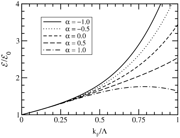
FIG. 8.: Energy density for a dilute Fermi system with spin degeneracy $g=4$ through ${\cal O}(k_{\rm F}^{9})$ as a function of $k_{\rm F}/\Lambda$, normalized to the energy density ${\cal E}_{0}$ for a free Fermi gas. The induced three-body contribution Eq. (51) is omitted for $\alpha\neq 0$. When it is included, all curves coincide with the $\alpha=0$ curve.

These cancellations manifest the invariance of finite density observables under field redefinitions. It is evident that one must include all induced terms. However, in past investigations with unitarily equivalent two-body potentials, possible induced three-body contributions were not considered. (As demonstrated in the next section, unitary transformations of the Hamiltonian have the same effect as field redefinitions.) Fig. 8 illustrates the consequence of omitting these terms for a dilute Fermi gas with spin degeneracy $g=4$. The energy density of the gas through ${\cal O}(k_{\rm F}^{9})$ (see [33] for details) is plotted for different values of $\alpha$, with the contributions ${\cal E}_{6(a)}$ and ${\cal E}_{6(b)}$ with two-body vertices included but the contribution ${\cal E}_{6(c)}$ with a three-body vertex not included. The result is a band of energies, analogous to the “Coester band” found for nuclear matter saturation curves [1]. The normalization of the transformation was chosen so that $\alpha=1$ is natural-sized; a manifestation is that the “correction” for $k_{\rm F}=\Lambda$ is order unity for $\alpha=1$. The spread of the Coester line curves in the medium is a measure of the natural size of three-body contributions.

In summary, we have used a simple field redefinition to illustrate how two-body off-shell vertices are induced but canceled exactly by new many-body vertices. Although we have worked to leading order in the EFT perturbation theory (that is, to leading order in a momentum expansion), the cancellation is guaranteed order-by-order. Next we show how unitary transformations on NN potentials exhibit the same behavior.

IV Unitary Transformations and Field Redefinitions

Infinitely many potentials that predict the same scattering phase shifts and energy spectrum can be constructed using unitary transformations [5]. If

$$H\Psi=(H_{0}+V)\Psi=E\Psi$$ (56)

and $\exp(iS)$ is a unitary operator of finite range:

$$e^{iS}\Psi=\widetilde{\Psi}\stackrel{{\scriptstyle\mathstrut r\rightarrow\infty}}{{\longrightarrow}}\Psi\ ,$$ (57)

then the transformed Hamiltonian

$$\widetilde{H}=e^{iS}He^{-iS}\equiv H_{0}+\widetilde{V}$$ (58)

has the same energy spectrum and phase shifts at all energies as $H$. The potentials $V$ and $\widetilde{V}$ are said to be phase-shift equivalent. Various practical methods to construct families of such potentials are described in the literature [1, 2, 3, 4, 5].

Here we demonstrate that these short-range unitary transformations have the same qualitative behavior as the simple field redefinitions in the last section: off-shell contributions are generated at the same time as compensating many-body contributions. This is only evident upon embedding the problem in a many-body framework from the beginning. The interplay between off-shell behavior and many-body forces in the context of unitary transformations has been studied in the literature [30, 31]. In particular, Ref. [30] proves a general theorem that guarantees the existence of three-body potentials that, when combined with unitarily equivalent two-body potentials, yield identical three-body observables.

We adapt the discussion of unitary transformations in Ref. [31], which addresses the key points (although we will use the notation of Ref. [40]). By writing the Hamiltonian and unitary operator in second-quantized form, the transformation becomes a canonical transformation of the creation and destruction operators. We consider spin-0 boson operators for simplicity; generalizing to spin-1/2 fermions is direct but would obscure the main points. We focus on a special case that highlights the relationship to local field redefinitions.

A Hamiltonian with kinetic energy and a two-body potential $V$ is written in terms of second-quantized field operators as [40]

$$\widehat{H}=\int\!d^{3}x\,\widehat{\psi}^{\dagger}({\bf x})\frac{-\overrightarrow{\nabla}^{2}\!}{2M}\widehat{\psi}({\bf x})+\frac{1}{2}\int\!\!\int\!d^{3}x\,d^{3}x^{\prime}\,\widehat{\psi}^{\dagger}({\bf x})\widehat{\psi}^{\dagger}({\bf x}^{\prime})V({\bf x},{\bf x}^{\prime})\widehat{\psi}({\bf x}^{\prime})\widehat{\psi}({\bf x})\ .$$ (59)

Amghar and Desplanques [31] consider unitary transformations of the form

$$\widehat{H}\longrightarrow e^{i{\widehat{S}}}\widehat{H}e^{-i{\widehat{S}}}=\widehat{H}+i[\widehat{S},\widehat{H}]+\cdots$$ (60)

with

$$\widehat{S}\equiv\int\!\!\int\!d^{3}x\,d^{3}x^{\prime}\,\widehat{\psi}^{\dagger}({\bf x})\widehat{\psi}^{\dagger}({\bf x}^{\prime})U({\bf x}-{\bf x}^{\prime})\widehat{\psi}({\bf x}^{\prime})\widehat{\psi}({\bf x})$$ (61)

and $U$ Hermitian. The simplest nontrivial form that maintains time-reversal invariance [31] is

$$U({\bf x})=\{{\bf p},{\bf x}f(x)\}=i\overleftarrow{\nabla}_{\!{\bf x}}\,{\bf x}f(x)+{\bf x}f(x)(-i)\overrightarrow{\nabla}_{\!{\bf x}}\,$$ (62)

where ${\bf p}$ is the momentum operator and the curly brackets denote an anti-commutator. They show that the transformation (60)–(62) generates two-body off-shell contributions but also many-body terms.

This transformation is nonlocal for a finite range $U$, which complicates the manipulations. If the nonlocality is of the order of the short-distance scale $\Lambda$, from an EFT perspective it is appropriate to replace $U({\bf x})$ with contact terms. That is, $U({\bf x})$ becomes proportional to a delta function with derivatives. The simplest choice is

$${\bf x}f(x)=\alpha\overrightarrow{\nabla}\delta^{3}({\bf x})\ .$$ (63)

where $\alpha$ is an arbitrary parameter. Since the interaction is singular, we can expect to generate divergent contributions, which we will regulate with dimensional regularization.

The transformation is most transparent in momentum space, with field expansions (in a box of volume $V$ with periodic boundary conditions) [40]:

$$\widehat{\psi}({\bf x})=\frac{1}{\sqrt{V}}\sum_{\bf k}e^{i{\bf k}\cdot{\bf x}}a^{\phantom{\dagger}}_{\bf k}\ ,\qquad\widehat{\psi}^{\dagger}({\bf x})=\frac{1}{\sqrt{V}}\sum_{\bf k}e^{-i{\bf k}\cdot{\bf x}}a^{\dagger}_{\bf k}\ ,$$ (64)

and boson commutation relations for the operators $a^{\phantom{\dagger}}_{\bf k}$ and $a^{\dagger}_{\bf k}$:

$$[a^{\phantom{\dagger}}_{\bf k},a^{\dagger}_{{\bf k}^{\prime}}]=\delta_{{\bf k}{\bf k}^{\prime}}\ ,\qquad[a^{\phantom{\dagger}}_{\bf k},a^{\phantom{\dagger}}_{{\bf k}^{\prime}}]=[a^{\dagger}_{\bf k},a^{\dagger}_{{\bf k}^{\prime}}]=0\ .$$ (65)

The Hamiltonian for a zero-range potential is

$$\widehat{H}=\sum_{{\bf k}}\frac{{\bf k}^{2}}{2M}\,a^{\dagger}_{\bf k}a^{\phantom{\dagger}}_{\bf k}+\frac{C_{0}}{2V}\sum_{{\bf k}_{1},{\bf k}_{2},{\bf k}_{3},{\bf k}_{4}}a^{\dagger}_{{\bf k}_{1}}a^{\dagger}_{{\bf k}_{2}}a^{\phantom{\dagger}}_{{\bf k}_{3}}a^{\phantom{\dagger}}_{{\bf k}_{4}}\delta^{\phantom{\dagger}}_{{\bf k}_{1}+{\bf k}_{2},{\bf k}_{3}+{\bf k}_{4}}\ ,$$ (66)

with $C_{0}$ given in Eq. (20). This Hamiltonian corresponds to the Lagrangian of Eq. (19) with the $C_{2}$ term omitted. In order to obtain the transformation operator $\widehat{S}$, we substitute Eqs. (62) and (63) into Eq. (61). After changing the integrations over $x$ and $x^{\prime}$ into integrations over $z_{\pm}=x\pm x^{\prime}$, the $z_{+}$ integration simply gives overall momentum conservation. The remaining integral can be carried out using a partial integration, and the transformation operator becomes

$$\widehat{S}=i\frac{\alpha}{4V}\sum_{{\bf k}_{1},{\bf k}_{2},{\bf k}_{3},{\bf k}_{4}}\Bigl{(}({\bf k}_{1}-{\bf k}_{2})^{2}-({\bf k}_{3}-{\bf k}_{4})^{2}\Bigr{)}\,a^{\dagger}_{{\bf k}_{1}}a^{\dagger}_{{\bf k}_{2}}a^{\phantom{\dagger}}_{{\bf k}_{3}}a^{\phantom{\dagger}}_{{\bf k}_{4}}\delta^{\phantom{\dagger}}_{{\bf k}_{1}+{\bf k}_{2},{\bf k}_{3}+{\bf k}_{4}}\ .$$ (67)

The transformed Hamiltonian is

$$\widehat{H}^{\prime} = \widehat{H}+i[\widehat{S},\widehat{H}]+{\cal O}(\alpha^{2})$$ (68)

$$= \widehat{H}+\frac{\alpha}{16MV}\sum_{{\bf k}_{1},{\bf k}_{2},{\bf k}_{3},{\bf k}_{4}}\Bigl{(}({\bf k}_{1}-{\bf k}_{2})^{2}-({\bf k}_{3}-{\bf k}_{4})^{2}\Bigr{)}^{2}\,a^{\dagger}_{{\bf k}_{1}}a^{\dagger}_{{\bf k}_{2}}a^{\phantom{\dagger}}_{{\bf k}_{3}}a^{\phantom{\dagger}}_{{\bf k}_{4}}\,\delta^{\phantom{\dagger}}_{{\bf k}_{1}+{\bf k}_{2},{\bf k}_{3}+{\bf k}_{4}}$$ (72)

$$-\frac{\alpha C_{0}}{2V^{2}}\sum_{{\bf k}_{1},{\bf k}_{2},{\bf k}_{3},{\bf k}_{4},{\bf k}_{5}}\Bigl{(}({\bf k}_{1}-{\bf k}_{2})^{2}-(2{\bf k}_{5}-{\bf k}_{3}-{\bf k}_{4})^{2}\Bigr{)}\,a^{\dagger}_{{\bf k}_{1}}a^{\dagger}_{{\bf k}_{2}}a^{\phantom{\dagger}}_{{\bf k}_{3}}a^{\phantom{\dagger}}_{{\bf k}_{4}}\,\delta^{\phantom{\dagger}}_{{\bf k}_{1}+{\bf k}_{2},{\bf k}_{3}+{\bf k}_{4}}$$

$$-\frac{\alpha C_{0}}{2V^{2}}\sum_{{\bf k}_{1},{\bf k}_{2},{\bf k}_{3},{\bf k}_{4},{\bf k}_{5},{\bf k}_{6}}\Bigl{(}({\bf k}_{1}-{\bf k}_{2})^{2}-({\bf k}_{4}-{\bf k}_{5}-{\bf k}_{6}+{\bf k}_{3})^{2}+({\bf k}_{4}-{\bf k}_{5})^{2}$$

$$\quad-({\bf k}_{1}-{\bf k}_{2}-{\bf k}_{3}+{\bf k}_{6})^{2}\Bigr{)}\,a^{\dagger}_{{\bf k}_{1}}a^{\dagger}_{{\bf k}_{2}}a^{\dagger}_{{\bf k}_{3}}a^{\phantom{\dagger}}_{{\bf k}_{4}}a^{\phantom{\dagger}}_{{\bf k}_{5}}a^{\phantom{\dagger}}_{{\bf k}_{6}}\,\delta^{\phantom{\dagger}}_{{\bf k}_{1}+{\bf k}_{2}+{\bf k}_{3},{\bf k}_{4}+{\bf k}_{5}+{\bf k}_{6}}+{\cal O}(\alpha^{2})$$

The two-body term generated from the commutator with the potential contains a divergent sum over the momentum ${\bf k}_{5}$. However, this is a pure power divergence, which is zero in dimensional regularization (with a cut-off regulator, it would simply renormalize the $C_{0}$ coefficient in the effective Lagrangian).

We observe that the momentum dependence of the first two-body term, which results from the commutator with the kinetic term, can be written

$$({\bf k}_{1}-{\bf k}_{2})^{2}-({\bf k}_{3}-{\bf k}_{4})^{2}=2({\bf k}_{1}^{2}+{\bf k}_{2}^{2}-{\bf k}_{3}^{2}-{\bf k}_{4}^{2})\ .$$ (73)

This factor vanishes for on-shell legs and so does not contribute to two-body scattering. The analysis proceeds in parallel with the analysis in the last section; we find the analog of Fig. 3 with the same result: the off-shell and three-body contributions cancel for $3\to 3$ scattering or in the medium.

We can identify a local field redefinition equivalent to this unitary transformation by directly transforming the field operator:

$$\widehat{\psi}({\bf x})\longrightarrow e^{i\widehat{S}}\widehat{\psi}({\bf x})e^{-i\widehat{S}}=\widehat{\psi}({\bf x})+i[\widehat{S},\widehat{\psi}({\bf x})]+{\cal O}(\alpha^{2})\ .$$ (74)

The commutator is conveniently evaluated by expanding in the momentum basis, Eq. (64), and using the commutation relations, Eq. (65). The end result can then be interpreted as a field redefinition in the effective Lagrangian:

$$\psi\longrightarrow\psi+\alpha\Bigl{[}(\overrightarrow{\nabla}^{2}\!\psi^{\dagger})\psi\psi+\psi^{\dagger}(\overrightarrow{\nabla}\psi)^{2}+(\overrightarrow{\nabla}\psi^{\dagger})\cdot\overrightarrow{\nabla}(\psi\psi)\Bigr{]}+{\cal O}(\alpha^{2})\ ,$$ (75)

with the corresponding redefinition of ${\psi^{\dagger}}$. This transformation generates a vertex equivalent to the term proportional to $\alpha/(MV)$ in Eq. (72) but also appears to generate a vertex with time-derivatives from the term,

$$\Delta{\cal L}=\alpha\Bigl{[}\psi^{\dagger}\psi^{\dagger}(\overrightarrow{\nabla}^{2}\!\psi)+(\overrightarrow{\nabla}\psi^{\dagger})^{2}\psi\Bigr{]}(i\partial_{t}\psi)+\mbox{H.c.}\ ,$$ (76)

which does not appear in the transformed Hamiltonian. However, the Feynman rule for this vertex is proportional to $\omega_{1}+\omega_{2}-\omega_{3}-\omega_{4}$, which vanishes identically by energy conservation.

In Ref. [41], EFT at finite density was explored by studying a perturbative matching example. In particular, a model potential

$$\langle{\bf k^{\prime}}|\hat{V}_{\rm true}|{\bf k}\rangle=\frac{4\pi}{M}\frac{\gamma m^{3}}{(k^{2}+m^{2})(k^{\prime}{}^{2}+m^{2})}\ .$$ (77)

was used to represent the underlying dynamics, where the mass $m$ corresponds to the range (and non-locality) of the potential; it plays the role of the underlying short-distance scale $\Lambda$. The dimensionless coupling $\gamma$ provides a perturbative expansion parameter. An EFT was introduced to reproduce observables in a double expansion: order-by-order in $\gamma$ as well as the EFT momentum expansion.

An effective $s$-wave potential in the form

$$\langle{\bf k^{\prime}}|\hat{V}_{\rm EFT}|{\bf k}\rangle=C_{0}+C_{2}\frac{\left(k^{2}+k^{\prime}{}^{2}\right)}{2}+C_{4}\frac{\left(k^{2}+k^{\prime}{}^{2}\right)^{2}}{4}+\widetilde{C}_{4}\frac{\left(k^{2}-k^{\prime}{}^{2}\right)^{2}}{4}+\ldots\ ,$$ (78)

was used. The EFT expansion of this potential was studied using both dimensional regularization and cut-off regularization. The term proportional to $\widetilde{C}_{4}$ does not contribute to on-shell two-body scattering in dimensional regularization, but is essential in the matching of the energy per particle in an infinite system. The value of $\widetilde{C}_{4}$ was determined by matching on-shell $3\to 3$ scattering in Ref. [41]. But it is tempting to conclude that this is merely equivalent to matching the T-matrices generated by Eqs. (77) and (78) off shell.

However, the unitary transformation discussed above shows that we can arbitrarily trade-off the value of $\widetilde{C}_{4}$ with the coefficient of a three-body contact term. This means that off-shell matrix elements of the potential (e.g., $\langle{\bf 0}|\hat{V}_{\rm EFT}|{\bf k}\rangle$) and subsequently the off-shell T-matrix can be changed continuously by varying $\alpha$, without changing any observables. One choice is to eliminate two-body off-shell vertices such as $\widetilde{C}_{4}$ entirely in favor of many-body vertices that do not vanish on shell. This is the form of many-body EFT used in Ref. [33], which corresponds to Georgi’s “on-shell effective field theory” [18]. In different situations, different choices may be more efficient [42].

V Summary

The attitude in the mid-seventies about off-shell physics is summarized in the review article by Srivastava and Sprung [6]:

“A knowledge of the off-energy-shell behavior of the nucleon-nucleon interaction is basic to nuclear physics. The on-energy-shell information, however complete (which it is not), is not adequate to permit unambiguous calculation of the properties of systems of more than two nucleons. Any reasonable agreement with nuclear binding energy and other properties obtained by using different potential models without knowing the correct off-energy-shell behavior of the interaction is probably fortuitous and therefore not very meaningful. The results obtained with different potentials only rarely agree with each other.”

In contrast, effective field theories are determined completely by on-energy-shell information, up to a well-defined truncation error. In writing down the most general Lagrangian consistent with the symmetries of the underlying theory, many-body forces arise naturally. Even though they are usually suppressed at low energies, they enter at some order in the EFT expansion. These many-body forces have to be determined from many-body data. The key point is, however, that no off-energy-shell information is needed or experimentally accessible.

In principle, one could consider the formal problem of particles interacting via a definite two-body potential, valid for all energies. From a physical point of view, such a description has to break down at a certain energy, when, for example, the substructure of the particles can be resolved. Furthermore, such a scenario cannot correspond to QCD where three-body forces are present at a fundamental level. The EFT approach is ideally suited to deal with such a situation, because at low energies all sensitivity to the high-energy dynamics can be captured in a few low-energy constants.

The variation in observables calculated using the two-body parts only when short-range unitary transformations are performed gives an indication of the natural size of three-body contributions. Given the correspondence of unitary transformations and field redefinitions (as shown in the previous section), this statement is a simple consequence of naive dimensional analysis in the EFT. In cases where naive dimensional analysis fails, further investigation is needed.

The modern consensus is that at least three-body forces are required as supplements to the best phenomenological NN interactions; discrepancies between calculated and experimental binding energies for the triton have made this conclusion unavoidable. But the emphasis on the importance of reproducing the “correct” off-shell physics still persists. For example, in a recent review of the state-of-the-art Bonn nucleon-nucleon potential, differences in the off-shell behavior of the Bonn potential compared to other contemporary NN potentials are stressed [43]. The hope of using many-nucleon systems to decide on the “correct” off-shell potential also persists [44, 45]. Again, the EFT viewpoint is that all theories with consistent power counting must agree up to truncation errors.

We have noted several consequences of the freedom to perform field redefinitions:

• An effective Lagrangian with energy-independent effective potentials can always be used, by eliminating time derivatives with field redefinitions. However, it is sometimes numerically convenient to trade momentum dependence for energy dependence [7], or to retain time dependence when incorporating relativistic corrections [42].

• The Lagrangian can be restricted to on-shell vertices only (cf. Georgi’s “on-shell effective field theory” [18]). One advantage of this choice is that the maximal number of energy diagrams vanish (at zero temperature).

• One can choose to trade off-shell contributions for many-body forces. If minimizing many-body forces is desirable, then one could argue that adjusting off-shell behavior to achieve this end is optimal. However, fine tuning is required to reduce many-body contributions below their “natural” size.

Finally, we note that different regularizations will also yield very different potentials, with different off-shell behavior, but observables will agree.

Number Operator

The field transformation, Eq. (21), changes the number operator of the theory, which is defined as the time component of the Noether current associated with the phase transformation $\psi\to\exp(-i\phi)\psi$. In the untransformed theory, the number operator is simply $\widehat{N}={\psi^{\dagger}}\psi$. The number density $n_{0}$ for the free Fermi gas at $T=0$ is given by the Feynman diagram shown in Fig. 9(a), where the cross indicates the insertion of the number operator.

FIG. 9.: Finite Density: diagrams for the number operator.

Evaluation of the Feynman diagram gives

$$n_{0}=-g\lim_{\eta\to 0^{+}}\int\frac{d^{4}\widetilde{p}}{(2\pi)^{4}}iG_{0}(\widetilde{p})e^{i\eta p_{0}}=g\frac{k_{\rm F}^{3}}{6\pi^{2}}\,.$$ (79)

This density $n_{0}$ remains unchanged by interactions and $n\equiv n_{0}$, which can be understood as follows. All contributions from interactions have the form shown in Fig. 9(b), where the blob represents the remainder of a given Feynman diagram. The crucial point is that there are always two different propagators with the same momentum connected to the insertion of $\widehat{N}$. As a consequence, there is no simple pole in the time component of the corresponding momentum, and the contour integral over the time component vanishes. This argument is valid as long as there are no off-shell terms in the vertices that cancel one of the propagators in question.

After the field transformation, Eq. (21), the number operator acquires an additional term of ${\cal O}(\alpha)$ and becomes

$$\widehat{N}_{\alpha}={\psi^{\dagger}}\psi+\frac{4\pi\alpha}{\Lambda^{3}}2\left({\psi^{\dagger}}\psi\right)^{2}\,.$$ (80)

The expectation value of the number operator and the density, however, remain unchanged. We show this explicitly for the lowest order in $\alpha$. At order $\alpha$, we have only the two new Feynman diagrams shown in Figs. 9(c) and 9(d). The cross indicates an insertion of the part of the number operator that is ${\cal O}(1)$, while the tetragram denotes the part of the number operator that is ${\cal O}(\alpha)$. The triangle denotes the induced off-shell vertex (iii) (cf. Eq. (28)). The diagram 9(c) does not vanish from the general argument above because the off-shell vertex cancels one of the propagators connected to the insertion of $\widehat{N}$. Evaluating the two diagrams, we find

$$n_{\ref{fdnumber}(c)} = -g(g-1)\frac{4\pi\alpha}{\Lambda^{3}}\frac{k_{\rm F}^{6}}{36\pi^{4}}=-n_{\ref{fdnumber}(d)}\ .$$ (81)

Thus the contributions cancel and the density is unchanged to ${\cal O}(\alpha)$. Higher order contributions in $\alpha$ cancel in a similar way.

REFERENCES

- [1] F. Coester, S. Cohen, B. Day, and C.M. Vincent, Phys. Rev. C 1 (1970) 769.
- [2] M.K. Srivastava, P.K. Banerjee, and D.W.L. Sprung, Phys. Lett. 31B (1970) 499.
- [3] M.I. Haftel and F. Tabakin, Phys. Rev. C 3 (1971) 921.
- [4] J.E. Monahan, C.M. Shakin, and R.M. Thaler, Phys. Rev. C 4 (1971) 43.
- [5] H. Ekstein, Phys. Rev. 117 (1960) 1590.
- [6] M.K. Srivastava and D.W.L. Sprung, Adv. Nucl. Phys. 8 (1975) 121.
- [7] G. P. Lepage, “What is Renormalization?”, in From Actions to Answers (TASI-89), edited by T. DeGrand and D. Toussaint (World Scientific, Singapore, 1989); [nucl-th/9706029].
- [8] D.B. Kaplan, [nucl-th/9506035].
- [9] H. Georgi, Ann. Rev. Nucl. Part. Sci. 43 (1993) 209.
- [10] Proceedings of the Joint Caltech/INT Workshop: Nuclear Physics with Effective Field Theory, ed. R. Seki, U. van Kolck, and M.J. Savage (World Scientific, 1998).
- [11] Proceedings of the INT Workshop: Nuclear Physics with Effective Field Theory II, ed. P.F. Bedaque, M.J. Savage, R. Seki, and U. van Kolck (World Scientific, 2000).
- [12] U. van Kolck, Prog. Part. Nucl. Phys. 43 (1999) 337.
-
[13]
S.R. Beane, P.F. Bedaque, W.C. Haxton, D.R. Phillips,
and M.J. Savage,
[nucl-th/0008064]. -
[14]
R. Haag, Phys. Rev. 112 (1958) 669;
J.S.R. Chisholm, Nucl. Phys. 26 (1961) 469;
S. Kamefuchi, L. O’Raifeartaigh, and A. Salam, Nucl. Phys. 28 (1961) 529. - [15] S. Coleman, J. Wess, and B. Zumino, Phys. Rev. 177 (1969) 2239.
- [16] M.C. Bergère and Y.-M.P. Lam, Phys. Rev. D 13 (1976) 3247.
- [17] H.D. Politzer, Nucl. Phys. B 172 (1980) 349.
- [18] H. Georgi, Nucl. Phys. B 361 (1991) 339.
- [19] W. Kilian and T. Ohl, Phys. Rev. D 50 (1994) 4649.
- [20] S. Scherer and H.W. Fearing, Phys. Rev. D 52 (1995) 6445.
- [21] C. Arzt, Phys. Lett. B 342 (1995) 189.
- [22] A.V. Manohar, in Ref. [10].
- [23] H.W. Fearing, Phys. Rev. Lett. 81 (1998) 758.
- [24] H.W. Fearing and S. Scherer, Phys. Rev. C 62 (2000) 034003.
- [25] S. Scherer and H.W. Fearing, Phys. Rev. C 51 (1995) 359.
- [26] J.L. Friar, D. Hüber, and U. van Kolck, Phys. Rev. C 59 (1999) 53.
- [27] T.D. Cohen, J.L. Friar, G.A. Miller, and U. van Kolck, Phys. Rev. C 53 (1996) 2661.
- [28] D. B. Kaplan, M. J. Savage, and M. B. Wise, Phys. Rev. C 59 (1999) 617.
- [29] I.R. Afnan and F.J.D. Serduke, Phys. Lett. 44B (1973) 143.
- [30] W.N. Polyzou and W. Glöckle, Few Body Syst. 9 (1990) 97.
- [31] A. Amghar and B. Desplanques, Nucl. Phys. A 585 (1995) 657.
- [32] P.F. Bedaque, H.-W. Hammer, and U. van Kolck, Nucl. Phys. A 676 (2000) 357; Nucl. Phys. A 646 (1999) 444; Phys. Rev. Lett 82 (1999) 463.
- [33] H.-W. Hammer and R.J. Furnstahl, Nucl. Phys. A678 (2000) 277, [nucl-th/0004043].
- [34] S. Coleman, Aspects of Symmetry (Cambridge Univ. Press, New York, 1988).
- [35] M. Bando, T. Kugo, K. Yamawaki, Phys. Rept. 164 (1988) 217.
- [36] J.F. Donoghue, E. Golowich, B.R. Holstein, Dynamics of the Standard Model (Campbridge Univ. Press, New York, 1992).
- [37] J. W. Negele and H. Orland, Quantum Many-Particle Systems (Addison-Wesley, New York, 1988).
- [38] P.F. Bedaque and H.W. Grießhammer, Nucl. Phys. A 675 (2000) 601.
- [39] D.B. Kaplan, in Ref. [10].
- [40] A. L. Fetter and J. D. Walecka, Quantum Theory of Many-Particle Systems (McGraw–Hill, New York, 1971).
- [41] R. J. Furnstahl, J. V. Steele, and N. Tirfessa, Nucl. Phys. A 671 (2000) 396.
- [42] J.-W. Chen, G. Rupak, and M.J. Savage, Nucl. Phys. A 653 (1999) 386.
- [43] R. Machleidt, [nucl-th/0006014].
- [44] A. Polls, H. Müther, R. Machleidt, and M. Hjorth-Jensen, Phys. Lett. B 432 (1998) 1.
- [45] P. Doleschall and I. Borbély, Phys. Rev. C 62 (2000) 054004.