CRITICAL PHENOMENA IN FINITE SYSTEMS

Abstract

We discuss the dynamics of finite systems within molecular dynamics models. Signatures of a critical behavior are analyzed and compared to experimental data both in nucleus-nucleus and metallic cluster collisions. We suggest the possibility to explore the instability region via tunneling. In this way we can obtain fragments at very low temperatures and densities. We call these fragments quantum drops.

1 Introduction

The dynamics of a fragmenting finite system can be well modeled by Classical Molecular Dynamics (CMD). Of course in such studies we are not interested in reproducing the data coming from nucleus-nucleus, cluster-cluster or fullerene-fullerene collisions, which are strongly influenced by quantum features, but simply in the possibility that a finite (un)charged system “remembers” of a liquid to gas phase transition which occurs in the infinite case limit [1]. Classical particles interacting through a short range repulsive interaction and a longer range attractive one have an Equation of State (EOS) which resembles a Van Der Waals (VDW) [1, 2]. It is also well known that the Nuclear EOS resembles a VDW as well [3], thus classical studies of the instability region are quite justified in order to understand the finite size plus Coulomb effects.

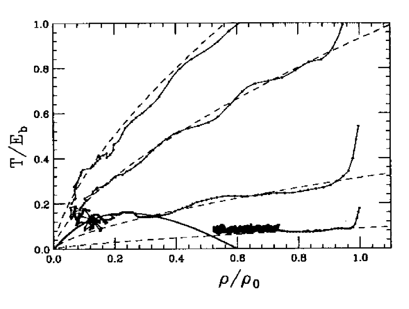
Figure 1: Time evolution of the biggest fragment in the density temperature plane.

Starting from a two body force, for instance of the Yukawa type, the EOS can be easily calculated within CMD using the virial theorem. This was done in ref.[1] and the resulting EOS spinodal line is plotted in Fig. 1 (full line) in the temperature $T$ density $\rho$ plane. These quantities have been normalized using typical values of the system. When dealing with phase transitions it is usual to normalize the various quantities by their values at the critical point of a second order phase transitions. Since later on, we will compare with some results on finite systems, where the values at the critical point (if it exist) are not known, we normalize by typical values in the ground state of the system such as density $\rho_{0}$, or the absolute value of the binding energy $E_{b}$. In such a way we can compare results coming from different systems such as nuclei or clusters [4].

Within CMD the time evolution of a finite and excited systems can be numerically calculated. In ref.[1] the time evolution of 100 particles was followed. The particles were initially given a Maxewell Boltzmann distribution at temperature $T$. The density and temperature estimated for the biggest fragment are plotted in Fig. 1 (full lines). Each dot is printed at regular time intervals of 1 fm/c. We have used a gs density for the finite system of $0.12{\rm fm}^{-3}$ ($0.15{\rm fm}^{-3}$ for the infinite case limit) and a B.E. of $-10$ MeV ($-16$ MeV in the infinite case) to normalize the curves. Without such normalizations the lowest curve ($T=2$ MeV) for instance will enter deeply inside the instability region which is not the case since this is a typical case of evaporation. “Critical” events occur for the initial $T=5$ MeV [1], which we see that enters into the instability region near the critical point for a second order phase transition. Note that the value of the excitation energy $E^{*}$ for this case is $E^{*}/E_{b}=0.71$, which coincides with the value of the $E^{*}/E_{b}$ obtained in the infinite case limit at the critical density and temperature. Some features in this figure are of interest. The first one is that the expansion is isentropic (dashed lines in Fig. 1) until the system enters the instability region; events at high $T$ do not enter the instability region, i.e. the system dissolves quickly because of the very large excitation energy. Already from these numerical experiments we understand that finite systems are quite different from the infinite limit case, in that there is no confining volume, thus $T$ and $\rho$ are time dependent quantities. Their values cannot be fixed from the outside but, to some extent the initial excitation energy and density can be fixed. The concept of temperature becomes questionable as well especially at high $E^{*}$. In fact the system expands rather quickly, and the very energetic particles leave the system without interacting with other particles. Thus fluctuations are small and decrease as we will show later with increasing $E^{*}$. Looking more carefully at Fig. 1, we notice that it is quite difficult to explore the instability region at small $T$. In fact in the case $T=2$ MeV the system is not able to enter the instability region. We need to give more excitation energy to it, but if we do so the $T$ when the system enters the instability region is larger. We can imagine to have a barrier in a collective space where the radial coordinate R and its conjugate momentum are the relevant degrees of freedom. Analogously to the process of spontaneous fission (SF) we can imagine that in presence of the long range Coulomb force, the barrier as a finite width, thus the quantum mechanical process of tunneling might be possible and the system enters the spinodal region at low $T$. We call the fragments thus formed quantum drops and discuss the process in a later section.

2 Observables

During a heavy ion collision many fragments are formed and finally detected. The first observable that was tested was the mass yield [5]. In fact from the Fisher model of phase transition we expect that if there is a phase transition, a power law should appear in the spectrum, see ref.[6]. In order to illustrate the Fisher model and to have a look at the modifications needed when dealing with a finite system we have repeated the calculations described above, each time changing randomly the momenta of the particles. In the simulation we can generate thousands of events and produce mass distributions at each $T$. The mass distribution so obtained is in good agreement with the Fisher law. The fits are rather good especially near and above the $T=5$ MeV case. The latter gives a very good power law distribution with $\tau=2.23$. Such a value of $\tau$ is in good agreement with what observed in liquid-gas phase transitions of finite systems. At very high $T$ the yield is practically exponentially decreasing, while low $T$ give one big fragment accompanied of some small ones. Other variables like moments of the mass distributions, Campi plots [7], give indications for a possible second order phase transition. In ref.[8] we have tested if these findings based on CMD results have some resemblance with reality. The experiment Au+Au at 35 MeV/A performed at MSU using the Multics-Miniball detectors [8] has been analyzed in terms of moments of mass distributions. First the collision was simulated in the framework of CMD and the effects of the experimental device were studied in detail [9]. It was found that a good reconstruction of the PLF can be obtained with this device. Thus peripheral collisions are rather well detected by the Multics-Miniball apparatus. For such collisions a critical behavior had been predicted within CMD in ref.[10] and confirmed for this system and at this energy as well [9, 11].

3 Chaotic Dynamics

The observation of large fluctuations in fragmentation hints to the occurrence of chaos. In order to address this problem quantitatively we calculate the maximal Lyapunov Exponents (MLE) as a function of the initial excitation energy. An important property of chaotic motion is the high sensibility to changes in the initial conditions. Closely neighboring trajectories diverge exponentially in time. For regular trajectories, on the other hand , they are found to diverge only linearly. The quantity that properly quantifies the rate of exponential divergence are the LE [12]. The MLE have been calculated in ref.[12] for the system of Fig. 1 and analogous calculations have been performed in ref.[13] within the Boltzmann Nordheim Vlasov (BNV) framework, i.e. a mean field description of a disassembling nucleus. In Fig. 2 the LE is plotted vs. excitation energy in the CMD (diamonds) and BNV case (squares). The qualitative behavior is the same, i.e. both calculations display a maximum at the normalized $E^{*}=0.5$.

Figure 2: Maximal Lyapunov exponents in CMD (diamonds) and BNV (squares) calculations.

Such maximum corresponds in the CMD to the value where the mass distribution is a power law. At low excitation energy the LE calculated in BNV are larger than the CMD case because the gs of the nucleus is a liquid while the classical gs is a solid. Very important is the decrease of the LE at high $E^{*}$. This clearly demonstrates that the degree of chaoticity, i.e. thermalization is not increasing and the initial excitation energy is partially thermal but a large amount is in the form of collective expansion. This is consistent with the picture of a limiting temperature that the nucleus can sustain [14]. In fact we can have a properly thermalized system when the self consistent field is able to bind the particles in some volume for some time. This field acts as a confining volume where the particles stay to boil. But, when the excitation energy is large, particles have enough kinetic energy to leave the system promptly. This picture greatly clarifies the dynamics of fragmentation. At low excitation energy we can have a liquid at a temperature $T$ which evaporates particles. At high $E^{*}$ energetic fragments are quickly emitted and a small liquid at a limiting $T$ remains. Thus the transition is from liquid to free particles thus somewhat different from a liquid to gas phase transition that would occur if the system was confined in a box.

4 Quantum Drops

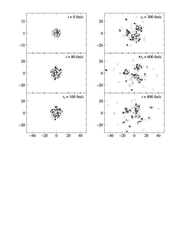
Figure 3: Time evolution of ${}^{238}U$ at 6.8 MeV/nucleon excitation energy. At time $t=100$ fm/c the system enters imaginary time and exits at $t=600$ fm/c. The real- and imaginary-times are indicated by $t$ and $t_{I}$.

Imagine that in some way we have been able to prepare the system at density $\rho$ and temperature $T$. Because of the compression and/or thermal pressure, the system will expand. If the excitation energy is too low the expansion will come to an halt and the system will shrink back. This is some kind of monopole oscillation. On the other hand if the excitation is very large it will quickly expand and reach a region where the system is unstable and many fragments are formed, cf. Fig. 1. It is clear that in the expansion process the initial temperature will also decrease. We could roughly describe this process with a collective coordinate $R(t)$, the radius of the system at time $t$ and its conjugate coordinate. Here we are simply assuming that the expansion is spherical. These coordinates are somewhat the counterpart of the relative distance between fragments in the fission process. Similarly to the fission process we can imagine that connected to the collective variable $R(t)$ there is a collective potential $V(R)$ [15]. When the excitation energy is too low it means that we are below the maximum of the potential. That such a maximum exists comes, exactly as in the fission process, from the short range nature of the nucleon-nucleon force and the long range nature of Coulomb. Thus, similarly to SF, we can imagine to reach fragmentation by tunneling through the collective potential $V(R)$. When this happens, fragments will be formed at very low $T$ not reachable otherwise than through the tunneling effect. The price to pay as in all the subbarrier phenomena is the very low cross sections. Since the expansion of the system can be parametrized in one-dimensional collective coordinate, we can, in principle, apply the imaginary-time method to its study similarly to ref.[15].

Here we combine the imaginary time prescription with Quantum Molecular Dynamics [16] model to simulate fragmentation of finite system with relatively low excitation. We simulate the expansion of ${}^{230}\rm U$ system. First we prepare the ground state of a nucleus and then compress uniformly to give an excitation energy $E^{*}$ from 5 to 8 MeV/nucleon. Due to the fluctuations between events caused by the different initial configuration of nucleus, the potential energy during the expansion is different for different events. Therefore the tunneling fragmentation occurs in some events where the potential energy is eventually high, while there is no tunneling for events with lower potential energy. The number of events with tunneling fragmentation is larger for lower excitation energy. In Fig. 3 we display snapshots of a typical tunneling event. The collective coordinate $P(t)$ becomes zero at $t=100$ fm/c. At this stage we turn to imaginary times and the tunneling begins. Notice that the system indeed expands and its shape can be rather well approximated to a sphere at the beginning. But already at 300 fm/c (in imaginary time) due to the molecular dynamics nature of the simulation, the spherical approximation is quite bad. This shortcoming of our approach should be kept in mind because the calculated action will be quite unrealistic due to the approximation used. This is similar to the use of one collective coordinate (the relative distance between centers) in SF process. In that case many calculated features are quantitatively wrong but qualitatively acceptable. Since our Quantum Drops is a proposed novel mechanism we can only give qualitative features and the model assumption must be refined when experimental data will start to be available [17].

5 Conclusions

Some theoretical indications for the behavior of a finite excited system are clear. Both CMD and BNV calculations of the MLE show that the system cannot hold more than a certain temperature. This seems intuitively reasonable because it is quite clear that the finite nuclear system is not able to stay bound when an excitation energy larger than 1.5$\sim$2 times the BE is given to it. It seems that at such large excitation energies, the systems quickly disassembles and consequently the biggest fragment left will have a lower excitation energy. The concept of a limiting temperature that the system can sustain seems reasonable, and such a limiting temperature is strictly related to the maximum value of the Lyapunov exponent . We propose also to search for fragmentation at very low excitation energies where quantum effects play a dominant role. These rare events should give valuable informations about the instability region.

References

References

- [1] V. Latora, M. Belkacem and A. Bonasera, Phys. Rev. Lett. 73,1765 (1994); M. Belkacem, V. Latora and A. Bonasera, Phys. Rev. C 52 (1995) 271; P. Finocchiaro, M. Belkacem, T. Kubo, V. Latora and A. Bonasera, Nucl. Phys. A600, 236 (1996).
-
[2]
L. Landau and E. Lifshits, Statistical Physics,
Pergamon, New York, 1980;
K.Huang, Statistical Mechanics, J.Wiley , New York, 1987, 2nd ed. - [3] A.L.Goodman, J. I. Kapusta and A. Z. Mekjian, Phys. Rev. C 30, 851 (1984).
- [4] A.Bonasera, Phys. World (Feb. 1999) 20. A. Bonasera and J. Schulte, contr. to the Proceedings Similarities and Differences between Atomic Nuclei and Clusters, et al. Abe et al. editors, AIP (1998).
- [5] M. L. Gilkes et al. Phys. Rev. Lett. 73, 1590 (1994).
- [6] M. E. Fisher, Proc. International School of Physics, Enrico Fermi Course LI, Critical Phenomena, ed. M. S. Green (Academic, New York, 1971); 1967255.
- [7] X. Campi, J. of Phys. A19, 917 (1986); Phys. Lett. B208, 351 (1988).
- [8] P. F. Mastinu et al. Phys.Rev.Lett. 76, 2646 (1996), and references therein.
- [9] M. Belkacem et al. Phys.Rev. C54, 2435 (1996).
- [10] V. Latora, A. Del Zoppo and A. Bonasera, Nucl. Phys. A572, 477 (1994).
- [11] A. Bonasera, M. Bruno, C. Dorso and P. F. Mastinu, Riv. Nuovo Cimento 23, 1-101 (2000).
- [12] A. Bonasera, V. Latora and A. Rapisarda, Phys. Rev. Lett. 75, 3434 (1995).
- [13] G. F. Burgio and A. Bonasera, in preparation.
- [14] K. Hagel et al., Phys. Rev. 62, 34607 (2000).
- [15] A. Bonasera and A. Iwamoto Phys. Rev. Lett. 78, 187 (1997).
- [16] T. Maruyama et al., Phys. Rev. 57, 655 (1998).
- [17] T. Maruyama, S. Chiba and A. Bonasera, in preparation.