DISCONTINUITIES IN RELATIVISTIC
HYDRODYNAMICS ACROSS SPACE-LIKE
AND TIME-LIKE HYPERSURFACES

Abstract

Discontinuities in relativistic hydrodynamics – shock waves and freeze-out shocks – are considered across both space-like and time-like hypersurfaces. We analyze the peculiar features of the freeze-out discontinuities and their connection to the shock-wave phenomena.

1. Hydrodynamical Discontinuities

Relativistic hydrodynamical model [1] has been widely discussed in recent years within their connection to high energy nucleus-nucleus (A+A) collisions (see, for example, [2]). The system evolution in relativistic hydrodynamics is governed by the energy-momentum tensor

$$T^{\mu\nu}~{}=~{}(\varepsilon+p)u^{\mu}u^{\nu}~{}-~{}pg^{\mu\nu}$$ (1)

and conserved charge currents. The baryonic current,

$$j^{\mu}~{}=~{}n~{}u^{\mu}~{},$$ (2)

plays the main role in the application to A+A collisions.

The hydrodynamical description includes the local thermodynamical variables (energy density $\varepsilon$, pressure $p$, baryonic density $n$) and the collective four-velocity $u^{\mu}=(1-{\bf v}^{2})^{-1/2}(1,{\bf v})$. The continuous flows are the solutions of the hydrodynamical equations

$$\partial_{\mu}T^{\mu\nu}~{}=~{}0~{},~{}~{}~{}~{}~{}\partial_{\mu}j^{\mu}~{}=~{}0~{},$$ (3)

with specified initial conditions.

Equations (3) are the differential form of the energy-momentum and baryonic number conservation laws. Along with these continuous flows, the conservation laws can also be realized in the form of discontinuous hydrodynamical flows which are called shock waves and satisfy the following equations:

$$T_{\rm o}^{\mu\nu}\Lambda_{\nu}=T^{\mu\nu}\Lambda_{\nu}\;\;,~{}~{}~{}~{}n_{{\rm o}}u_{{\rm o}}^{\mu}\Lambda_{\mu}=nu^{\mu}\Lambda_{\mu}\;\;,$$ (4)

where $\Lambda_{\mu}$ is the unit 4-vector normal to the discontinuity hypersurface. In Eq. (4) the zero subscript corresponds to the initial state ahead of the shock front and the quantities without an index are the final state values behind it. To complete the system of the hydrodynamical equations (3) or (4) the fluid equation of state (EoS) has to be added as an input $p=p(\varepsilon,n)$.

Besides the fluid EoS and the initial conditions for the fluid evolution the third crucial ingredient of the hydrodynamical model of A+A collisions is the so-called freeze-out (FO) procedure, i.e. the prescription for the calculations of the final hadron observables. Particles which leave the system and reach the detectors are considered via FO scheme, where the frozen-out particles are formed on a 3-dimensional hypersurface in space-time. The FO description has a straight influence on particle momentum spectra and therefore on all hadron observables. A generalization of the well known Cooper-Frye (CF) formula [3] to the case of time-like (t.l.) FO hypersurface was suggested in Ref. [4]. The new formula does not contain negative particle number contributions on t.l. FO hypersurface appeared in the CF procedure from those particles which cannot leave the fluid during its hydrodynamical expansion. The FO procedure of Ref. [4] has been further developed in a series of publications [5-10]. The particle emission from the t.l. parts of the FO hypersurface looks as a ‘discontinuity’ in the hydrodynamic motion. We call it the FO shock.

In the present paper we analyze the discontinuities in relativistic hydrodynamics – normal shock waves and the FO shocks – across both space-like (s.l.) and t.l. hypersurfaces.

2. Relativistic Shock Waves

The relativistic shock waves are defined by equations (4). The important constraint on the shock transitions (4) is the requirement of non-decreasing entropy (thermodynamical stability condition):

$$su^{\mu}\Lambda_{\mu}\geq s_{{\rm o}}u_{{\rm o}}^{\mu}\Lambda_{\mu}\;,$$ (5)

where $s$ is the entropy density.

We consider one-dimensional hydrodynamical motion in what follows. In its usual sense the theory of the shock waves corresponds to the discontinuities across the t.l. surface, i.e. the normal vector $\Lambda_{\mu}$ is a s.l. one. It means that the shock-front velocity is smaller than 1. In this case one can always choose the Lorentz frame where the shock front is at rest. Then the hypersurface of shock discontinuity is $x_{sh}=const$ and $\Lambda_{\mu}=(0,1)$. The shock equations (4) become

$$T_{{\rm o}}^{01}=T^{01},\;\;T_{{\rm o}}^{11}=T^{11}\;\;,~{}~{}~{}n_{{\rm o}}u_{{\rm o}}^{1}=nu^{1}\;\;.$$ (6)

From Eq. (6) one obtains

$$v_{{\rm o}}^{2}=\frac{(p-p_{{\rm o}})(\varepsilon+p_{{\rm o}})}{(\varepsilon-\varepsilon_{{\rm o}})(\varepsilon_{{\rm o}}+p)}\;,\;\;v^{2}=\frac{(p-p_{{\rm o}})(\varepsilon_{{\rm o}}+p)}{(\varepsilon-\varepsilon_{{\rm o}})(\varepsilon+p_{{\rm o}})}\;\;.$$ (7)

Substituting (7) into the last equation in (6) we obtain the well known Taub adiabate (TA) equation  [11]

$$n^{2}X^{2}-n_{{\rm o}}^{2}X_{{\rm o}}^{2}-(p-p_{{\rm o}})(X+X_{{\rm o}})=0\;\;,$$ (8)

in which $X\equiv(\varepsilon+p)/n^{2}$, and TA therefore contains only the thermodynamical variables.

The point $(\varepsilon_{{\rm o}},p_{{\rm o}},n_{{\rm o}})$ is called the center of the TA. The mechanical stability of the shock transition from the state $(\varepsilon_{{\rm o}},p_{{\rm o}},n_{{\rm o}})$ to $(\varepsilon,p,n)$ was studied in Refs. [12, 13]. Thermodynamical stability (5) follows from the mechanical stability, and the inverse statement is not in general true [12, 13]. The consequences of the mechanical stability are also the well-known inequalities for the speed of sound and the flow velocities at both sides of the shock front in its rest frame

$$c_{s{\rm o}}~{}\leq~{}v_{{\rm o}}~{},~{}~{}~{}~{}c_{s}~{}\geq~{}v~{}.$$ (9)

In the thermodynamically normal media the compression shocks are stable whereas the rarefaction shocks become stable in the thermodynamically anomalous media. The shock-wave stability in the case of the phase transitions between hadron matter and the quark-gluon plasma are discussed in Refs. [14, 15].

Let us consider now the discontinuities on a hypersurface with a t.l. normal vector $\Lambda_{\mu}$ (t.l. shocks). This new possibility was suggested by Csernai in Ref. [16]. In this case one can always choose another convenient Lorentz frame (’simultaneous system’) where the hypersurface of the discontinuity is $t_{sh}=const$ and $\Lambda_{\nu}=(1,0)$. Equations (4) become then

$$T_{{\rm o}}^{00}=T^{00},\;\;T_{{\rm o}}^{10}=T^{10}\;\;,~{}~{}~{}n_{{\rm o}}u_{{\rm o}}^{0}=nu^{0}\;\;.$$ (10)

From Eq. (10) we find

$$\tilde{v}_{{\rm o}}^{2}=\frac{(\varepsilon-\varepsilon_{{\rm o}})(\varepsilon_{{\rm o}}+p)}{(p-p_{{\rm o}})(\varepsilon+p_{{\rm o}})}~{},\;\;~{}~{}\tilde{v}^{2}=\frac{(\varepsilon-\varepsilon_{{\rm o}})(\varepsilon+p_{{\rm o}})}{(p-p_{{\rm o}})(\varepsilon_{{\rm o}}+p)}\;\;,$$ (11)

where we use $``\sim"$ sign to distinguish the t.l. shock case (11) from the standard s.l. shocks (7). Substituting (11) into the last equation in (10) one finds the equation for t.l. shocks which is identical to the TA of Eq. (8). We stress, however, that the intermediate steps are quite different. The two solutions, Eqs. (11) and (7), are connected to each other by simple relations,

$$\tilde{v}_{{\rm o}}^{2}=\frac{1}{v_{{\rm o}}^{2}}~{},\;\;~{}~{}\tilde{v}^{2}=\frac{1}{v^{2}}\;\;,$$ (12)

between the velocities of s.l. and t.l. shocks. These relations show that only one type of transitions can be realized for the given initial and final states. Physical regions $[0,1)$ for $v_{{\rm o}}^{2},v^{2}$ (7) and for $\tilde{v}_{{\rm o}}^{2},\tilde{v}^{2}$ (11) in the $(\varepsilon$–$p)$-plane are shown in Fig. 1.

When the initial and final states are thermodynamically equilibrated the TA passes through the point $(\varepsilon_{{\rm o}},p_{{\rm o}})$ and lies as a whole in the regions I and IV in Fig.  1 [13], i.e. only compression and/or rarefaction s.l. shocks (with s.l. normal vector $\Lambda_{\mu}$) are permitted.

The only way to make the t.l. shocks to be possible is to allow the metastable initial and/or final states. Then new possibilities of t.l. shock transitions (10,11) to regions III and VI in Fig. 1 would be realized (see, e.g., the t.l. shock hadronization of the supecooled quark-gluon plasma in Ref. [17]).

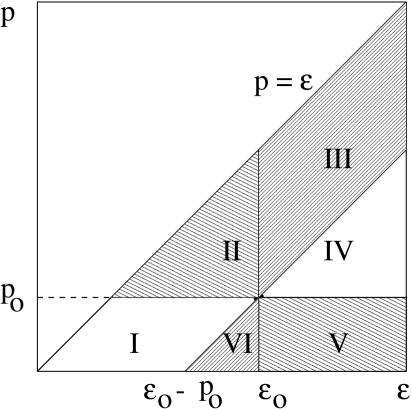
Fig. 1.: Possible final states in the $\varepsilon-p$ plane for shock transitions from the initial state $(\varepsilon_{{\rm o}},p_{{\rm o}}$). I and IV are the physical regions for s.l. shocks, III and VI for t.l. shocks. II and V are unphysical regions for both types of shocks. Note, that only states with $p\leq\varepsilon$ are possible for any physical equation of state in relativistic theory.

3. Freeze Out Shocks

In the hydrodynamical model of A+A collisions the fluid expansion has to be ended by the correct transformation of the fluid into free streaming hadrons. The most important requirement for this FO procedure is to satisfy energy-momentum and charge conservations during the fluid transition into free final particles. It is assumed that there is a narrow space-time region where the mean free path of the fluid constituents increases rapidly and becomes comparable with the characteristic size of the system. The local thermal equilibrium is supposedly maintained in this intermediate region. In practice, one considers a “zero width” approximation and introduces a FO surface, so that particle distributions remain frozen-out from there on.

In his original paper Landau [1] defined the FO hypersurface by the condition $T(t,x)=T^{*}$, where $t$ and $x$ are the time and the space coordinate respectively, and $T^{*}$ is the fluid FO temperature chosen to be approximately equal to the pion mass. The FO procedure, first introduced by Milekhin [19], was improved further by Cooper and Frye [3] and this method has been used ever since. Final momentum spectra for i-th type hadrons are expressed by the formula [3]:

$$k^{{\rm o}}\frac{d^{3}N_{i}}{dk^{3}}~{}=~{}\frac{d_{i}}{(2\pi)^{3}}\int_{\Sigma_{f}}d\sigma_{\mu}k^{\mu}~{}\phi_{i}\left(\frac{k^{\nu}u_{\nu}-\mu_{i}}{T^{*}}\right)~{},$$ (13)

where $d\sigma_{m}u$ is the external normal 4-vector to the FO hypersurface $\Sigma_{f}$. It equals to $S_{tr}(-dx,dt)$ in 1+1 dimension, where $S_{tr}$ is the (constant) transverse area of the system. $\phi_{i}$ denotes the local thermal Bose or Fermi distributions, $d_{i}$ is the degeneracy factor for particle $i$ with the chemical potential $\mu_{i}$. The particle spectrum (13) is known as the CF distribution function.

The initial conditions of the hydrodynamical motion are given on the initial (s.l.) hypersurface $\Sigma_{in}$. The final hypersurface $\Sigma_{f}$ should be closed to $\Sigma_{in}$ and in general $\Sigma_{f}$ consists of both s.l. and t.l. parts. The CF formula(13) leads automatically to the energy-momentum and charge number conservations, if the ideal gas fluid EoS at the FO hypersurface is assumed.

The CF formula (13) still does not provide a complete solution of the FO problem. The FO surface consists of t.l. parts too. Eq. (13) can not however be used for a t.l. FO surface (i.e., s.l. normal vector $d\sigma_{\mu}$): free final particles “return” to the fluid if $d\sigma_{\mu}k^{\mu}<0$, and this causes unphysical negative contributions to the number of final particles. The modified FO procedure and new formula for the final particle spectra emitted from the t.l. FO hypersurface was proposed in Ref. [4]:

$$k^{{\rm o}}\frac{d^{3}N_{i}}{dk^{3}}~{}=~{}\frac{d_{i}}{(2\pi)^{3}}\int_{\Sigma_{f}}d\sigma_{\mu}k^{\mu}~{}\phi_{i}\left(\frac{k_{\lambda}u^{\lambda}_{g}-\mu_{i}^{g}}{T_{g}}\right)~{}\theta(d\sigma_{\nu}k^{\nu})~{}.$$ (14)

Eq. (14) looks like CF formula (13), but without negative particle numbers that appear in (13) for t.l. FO surfaces. These negative contributions are cut-off by the $\theta$-function in Eq. (14). We’ll call Eq. (14) the cut-off (CO) distribution in what follows. An inclusion of the CO FO into the self-consistent hydrodynamical scheme is considered in Ref. [10]. The distribution function for the free particles in Eq. (14) contains the new parameters $T_{g},\mu_{i}^{g},u^{\nu}_{g}$. We’ll briefly call the free particle state as the ‘gas’ in order to distinguish it from the ordinary fluid. Note, however, that final particle system differs from the normal fluid and gas. It has the non-thermal CO distribution function which is frozen-out as all further particle rescatterings are ‘forbidden’ in the post-FO gas state.

The presence of the $\theta$-function in the right hand side of Eq. (14) leads to the discontinuity between the fluid $T_{f},\mu_{i}^{f},u^{\nu}_{f}$ and the gas $T_{g},\mu_{i}^{g},u^{\nu}_{g}$ variables across the t.l. FO hypersurface to satisfy the energy-momentum and charge conservations. We call this discontinuity the FO shock.

Let us consider this FO shock on t.l. hypersurface in more detail. To obtain the analytical solution of the problem we restrict ourself to the case of zero baryonic number $n=0$ and consider massless particles with the Jüttner distribution function

$$\phi\left(\frac{k_{\mu}u^{\mu}}{T}\right)~{}=~{}\exp\left(-~{}\frac{k_{\mu}u^{\mu}}{T}\right)~{}.$$ (15)

The energy-momentum conservation between the fluid and free particles along the t.l. hypersurface acquires the form:

$$~{}d\sigma_{\mu}T^{\mu\nu}_{f}\equiv\frac{d\sigma_{\mu}}{(2\pi)^{3}}\int\frac{d^{3}k}{k^{{\rm o}}}~{}k^{\mu}k^{\nu}~{}\phi\left(\frac{k_{\nu}u^{\nu}_{f}}{T_{f}}\right)~{}=$$ (16)

$$= ~{}d\sigma_{\mu}T^{\mu\nu}_{g}~{}\equiv\frac{d\sigma_{\mu}}{(2\pi)^{3}}\int\frac{d^{3}k}{k^{{\rm o}}}~{}k^{\mu}k^{\nu}~{}\phi\left(\frac{k_{\nu}u^{\nu}_{g}}{T_{g}}\right)~{}\theta(d\sigma_{\lambda}k^{\lambda})~{}.$$

The energy-momentum tensor $T^{\mu\nu}_{f}$ in Eq. (16) has the form of Eq. (1) with the functions $\varepsilon(T_{f})=\varepsilon_{f}$ and $p(T_{f})=p_{f}$ given by

$$\varepsilon(T)~{}=~{}3p(T)~{}=~{}\frac{1}{2\pi^{2}}\int_{0}^{\infty}k^{2}dk~{}k~{}~{}\exp\left(-\frac{k}{T}\right)~{}=~{}\frac{3}{\pi^{2}}~{}T^{4}~{}.$$ (17)

In the rest frame of the FO front, i.e. in the Lorentz frame where $d\sigma_{\mu}$ becomes equal to $S_{tr}(0,dt)$, the $T^{01}_{g}$ and $T^{11}_{g}$ components of the gas energy-momentum tensor in Eq. (16) can be rewritten then in the form

$$T^{01}_{g}~{}=~{}(\varepsilon^{*}_{g}+p^{*}_{g})u^{0}_{g}u^{1}_{g}~{},~{}~{}~{}~{}T^{11}_{g}~{}=~{}(\varepsilon^{*}_{g}+p^{*}_{g})u^{1}_{g}u^{1}_{g}~{}+p^{*}_{g}~{}.$$ (18)

It also coincides with that of Eq. (1), but with effective values of $\varepsilon^{*}_{g}$ and $p^{*}_{g}$ which are found to be equal to

$$\varepsilon_{g}^{*}~{}=~{}\varepsilon(T_{g})~{}\frac{(1+v_{g})^{2}}{4v_{g}}~{},~{}~{}~{}~{}p^{*}_{g}~{}=~{}p(T_{g})~{}\frac{(1+v_{g})^{2}(2-v_{g})}{4}~{},$$ (19)

where $v_{g}$ is the velocity parameter of the gas in the FO shock rest frame. The functions $\varepsilon$ and $p$ in the right hand side of Eqs. (19) are given by Eq. (17).

Due to the same formal structure of $T^{01}_{g},T^{11}_{g}$ (18) and $T^{01}_{f},T^{11}_{f}$ (1) one obtains the solution of Eq. (16)

$$v_{f}^{2}=\frac{(p_{f}-p_{g}^{*})(\varepsilon_{g}^{*}+p_{f})}{(\varepsilon_{f}-\varepsilon_{g}^{*})(\varepsilon_{f}+p_{g}^{*})}\;,\;\;~{}~{}v_{g}^{2}=\frac{(p_{f}-p^{*}_{g})(\varepsilon_{f}+p^{*}_{g})}{(\varepsilon_{f}-\varepsilon^{*}_{g})(\varepsilon^{*}_{g}+p_{f})}~{},$$ (20)

which is similar to Eq. (7). Note, however, that in contrast to Eq. (7) the values of $\varepsilon_{g}^{*}$ and $p_{g}^{*}$ in Eq. (20) are not just the thermodynamical quantities, but depend also on $v_{g}$.

It should be emphasized that Eq. (18) can also be introduced for the distribution functions of massive and charged particles [10]. In the latter case the energy-momentum conservation leads to the familiar expressions (20) for the effective energy density and pressure, and the charge conservation leads to the TA equation (8) for the effective charge density.

We fix the FO hypersurface $\Sigma_{f}$ by the condition $T_{g}=const$. The analytical solution of Eq. (20) can be presented then in the form

$$v_{g}~{}=~{}\frac{9v_{f}^{2}-8v_{f}+3}{3v_{f}^{2}+1}~{},~{}~{}~{}~{}R~{}\equiv~{}\left(\frac{T_{f}}{T_{g}}\right)^{4}~{}=~{}\frac{4(3v_{f}^{2}-2v_{f}+1)^{2}(v_{f}+1)}{(3v_{f}-1)(3v_{f}^{2}+1)^{2}}~{}.$$ (21)

It is instructive to compare these results with shock-wave solution (7) for the same ideal gas EoS (17). We fix the temperature $T_{g}$ of the final state in s.l. shock wave (6) and consider $v_{g}$ and $T_{f}$ dependence on $v_{f}$:

$$v_{g}~{}=~{}\frac{1}{3v_{f}}~{},~{}~{}~{}~{}R~{}\equiv~{}\left(\frac{T_{f}}{T_{g}}\right)^{4}~{}=~{}\frac{3(1-v_{f}^{2})}{9v_{f}^{2}-1}~{}.$$ (22)

Figs. 2 and 3 show the dependences of $v_{g}$ and $T_{f}$ on $v_{f}$ for the fixed temperature $T_{g}$ in the final state, both for the FO shock (21) and for the normal shock wave (22). The kinematical restrictions on the gas velocity give the same value of the minimal fluid velocity in both shock transitions, $(v_{f})_{min}=p_{f}/\varepsilon_{f}$. It equals to $1/3$ for the considered ideal gas EoS (17) of the fluid. Figs. 2 and 3 indicate that at low values of the fluid velocity, $v_{f}<1/\sqrt{3}$, the behavior of $v_{f}$ and $T_{f}/T_{g}$ for the FO shock (21) and for the normal shock wave (22) is quite similar. The value of $v_{f}=1/\sqrt{3}$ corresponds to the speed of sound, $c_{s}=1/\sqrt{3}$, in the system with ideal gas EoS (17). According to the requirements given by Eq. (9) the shock transitions at $v_{f}<c_{s}$ are mechanically unstable. Mechanically stable solutions at $v_{f}>c_{s}$ for normal shock waves and FO shocks have qualitatively different behavior. For the stable normal shock wave one has $v_{g}<v_{f}$ and $T_{f}<T_{g}$ (see Figs. 2, 3), i.e. only compression normal shock wave transitions ’f ’$\rightarrow$’g ’ would be stable. For the FO shock transitions we find a completely different behavior, $v_{g}>v_{f}$ and $T_{f}>T_{g}$, illustrated in Figs. 2, 3. In contrast to the normal shock waves, only the rarefaction FO shock transitions ’f ’$\rightarrow$’g ’ are stable. This result is in agreement with an intuitive physical picture of the FO as a rarefaction process.

Fig. 2.: Gas velocity $v_{g}$ as a function of the fluid velocity $v_{f}$ in the rest frame of the shock front. The dashed lines represent mechanically unstable transitions, whereas the solid lines show the mechanically stable FO shocks and normal shock waves. Thin lines correspond to a normal shock wave (Eq. (22)) and the thick ones correspond to the freeze-out shock (Eq. (21)). The circle has the coordinates $(1/\sqrt{3};3-4/\sqrt{3})$ and the square has the coordinates $(1/\sqrt{3};1/\sqrt{3})$.

The entropy flux of the fluid is given by

$$s_{f}^{\mu}d\sigma_{\mu}~{}=~{}s_{f}u_{f}^{\mu}d\sigma_{\mu}~{},$$ (23)

where $s_{f}=(\varepsilon_{f}+p_{f})/T_{f}$ is the fluid entropy density. Similar expression is valid for the final ’gas’ state in the case of normal shock waves. The entropy production in the normal shock waves is given by the formula

$$\frac{s_{g}^{\mu}d\sigma_{\mu}}{s_{f}^{\mu}d\sigma_{\mu}}~{}=~{}\frac{1}{3^{3/4}v_{f}}\left[\frac{9v_{f}^{2}-1}{1-v_{f}^{2}}\right]^{1/4}\,\,$$ (24)

and is shown in Fig. 4. The entropy flux of the gas with the cut-off distribution function is given by [10]:

$$s_{g}^{\mu}d\sigma_{\mu}~{}=~{}\frac{d\sigma_{\mu}}{(2\pi)^{3}}\int\frac{d^{3}k}{k^{{\rm o}}}~{}k^{\mu}~{}\phi\left(~{}\frac{k_{\nu}u^{\nu}_{g}}{T_{g}}\right)\left[~{}1~{}-~{}\ln~{}\phi\left(~{}\frac{k_{\nu}u^{\nu}_{g}}{T_{g}}\right)\right]\theta(d\sigma_{\lambda}k^{\lambda})~{}.$$ (25)

The entropy production in the FO shocks is calculated then as

$$\frac{s_{g}^{\mu}d\sigma_{\mu}}{s_{f}^{\mu}d\sigma_{\mu}}~{}=~{}\frac{1}{2v_{f}}\left[\frac{(3v_{f}^{2}+1)^{2}(3v_{f}-1)}{(1+v_{f})}\right]^{1/4}\,\,.$$ (26)

The maximal entropy production in the FO shock (26) corresponds to $v_{f}=c_{s}=1/\sqrt{3}$ and can be considered as an analog of the Chapman–Jouguet point (see Fig. 4).

Fig. 3.: Ratio of the temperatures on the both sides of the shock front, $T_{f}/T_{g}$, as a function of the fluid velocity $v_{f}$ in the rest frame of the shock front. The legend corresponds to the Fig. 2. The circle has the coordinates $\left[1/\sqrt{3};(8/(3\sqrt{3}))^{1/4}\right]$ and the square has the coordinates $(1/\sqrt{3};1)$.

4. Conclusions

In the present paper the discontinuities in relativistic hydrodynamics have been considered. The particle emission from t.l. parts of the FO hypersurface looks as a discontinuity in the hydrodynamical motion (FO shocks). The connection of these FO shocks to the normal shock waves in the relativistic hydrodynamics has been analyzed. The above consideration can be used in the hydrodynamical approach to the relativistic A+A collisions. It should be also important in the models of A+A collisions which combine hydrodynamics for the early stage of the reaction with a microscopic hadron description of the later stages (see, for example, Ref. [20]).

AcknowledgmentAuthors thank D.H. Rischke and G. Yen for useful discussions. M.I.G. acknowledges the financial support of DFG, Germany. K.A.B. is grateful to the Alexander von Humboldt Foundation for the financial support.

Fig. 4.: Ratio of the entropies on the both sides of the shock front, as a function of the fluid velocity $v_{f}$ in the rest frame of the shock front. The legend corresponds to the Fig. 2. The circle corresponds to the maximal entropy (analog of the Chapman-Jouguet point) in the freeze-out shock and it has the coordinates $\left[1/\sqrt{3};\left(\frac{9(3-\sqrt{3})}{4(\sqrt{3}+1)}\right)^{1/4}\right]$ and the square has the coordinates $(1/\sqrt{3};1)$.

References

- [1] L.D. Landau, Izv. Akad. Nauk SSSR 17 (1953) 51.
-
[2]
H. Stöcker and W. Greiner, Phys. Rep. 137 (1986) 277;
R.B. Clare and D.D. Strottman, Phys. Rep. 141 (1986) 177;
D. H. Rischke, Proceedings of the 11th Chris Engelbrecht Summer School in Theoretical Physics, “Hadrons in Dense Matter and Hadrosynthesis”, Cape Town, South Africa, Febr. 4 – 13, 1998 (Springer, Berlin), p. 21ff; Preprint nucl-th/9809044. - [3] F. Cooper and G. Frye,Phys. Rev. D 10 (1974) 186.
- [4] K.A. Bugaev, Nucl. Phys. A 606 (1996) 559.
- [5] J.J. Neumann, B. Lavrenchuk and G. Fai, Heavy Ion Physics 5 (1997) 27.
- [6] L.P. Csernai, Z. Lázár and D. Molnár, Heavy Ion Physics 5 (1997) 467.
- [7] Cs. Anderlik, L.P. Csernai, F. Grassi, Y. Hama, T. Kodama and Zs. Lázár, Preprint nucl-th/9806004.
- [8] Cs. Anderlik, Zs. Lázár, V.K. Magas, L.P. Csernai, H. Stöcker and W. Greiner, Phys. Rev. C 59 (1999) 1.
- [9] V. Magas, “Freeze out in hydrodynamical models”, Master of Science Thesis, University of Bergen, January 1999.
- [10] K.A. Bugaev and M.I. Gorenstein, Preprint nucl-th/9903072.
- [11] A.H. Taub, Phys. Rev. 74 (1948) 328.
-
[12]
M.I. Gorenstein and V.I. Zhdanov, Z. Phys. C 34 (1987) 79;
K.A. Bugaev and M.I. Gorenstein, J. Phys. G 13 (1987) 1231;
K.A. Bugaev and M.I. Gorenstein, Z. Phys. C 43 (1989) 261. - [13] K.A. Bugaev, M.I. Gorenstein and V.I. Zhdanov, Z. Phys. C 39 (1988) 365.
- [14] K.A. Bugaev, M.I. Gorenstein, B. Kämpfer and V.I. Zhdanov, Phys. Rev. D 40 (1989) 2983.
- [15] K.A. Bugaev, M.I. Gorenstein and D.H. Rischke, Phys. Lett. B 255 (1991) 18; JETP Pis’ma (Russ.) 52 (1990) 1121.
- [16] L. Csernai, Zh. Eksp. Teor. Fiz. (Russ.) 92 (1987) 379; Sov. Phys. JETP 65 (1987) 216.
-
[17]
T. Csörgö and L.P. Csernai, Phys. Lett. B 333 (1994) 494.
M.I. Gorenstein, H.G. Miller, R.M. Quick and R.A. Ritchie, Pyhs. Lett. B 340 (1994) 109. - [18] K.A. Bugaev, “Rarefaction Shocks in Quark Baryonic Matter Hadronization”, Preprint ITP-88-169P, Kiev (1989) 11 p.
- [19] G.A. Milekhin, Zh. Eksp. Teor. Fiz. 35 (1958) 1185; Sov. Phys. JETP 35 (1959) 829; Trudy FIAN 16 (1961) 51.
- [20] S.A. Bass et al., “Hadronic freeze-out following a first order hadronization in ultrarelativistic heavy-ion collisions”, Preprint nucl-th/9902062 (1999).