Local Energy–Density Functional Approach to
Many–Body Nuclear Systems with S–Wave Pairing

Abstract

The ground-state properties of superfluid nuclear systems with ${}^{1}S_{0}$ pairing are studied within a local energy-density functional (LEDF) approach. A new form of the LEDF is proposed with a volume part which fits the Friedman-Pandharipande and Wiringa-Fiks-Fabrocini equation of state at low and moderate densities and allows an extrapolation to higher densities preserving causality. For inhomogeneous systems, a surface term is added, with two free parameters, which has a fractional form like a Padé approximant containing the gradient of density squared in both the numerator and denominator. In addition to the Coulomb direct and exchange interaction energy, an effective density-dependent Coulomb-nuclear correlation term is included with one more free parameter. A three-parameter fit to the masses and radii of about 100 spherical nuclei has shown that the latter term gives a contribution of the same order of magnitude as the Nolen-Schiffer anomaly in Coulomb displacement energy. The root-mean-square deviations from experimental masses and radii with the proposed LEDF come out about a factor of two smaller than those obtained with the conventional functionals based on the Skyrme or finite-range Gogny force, or on the relativistic mean-field theory. The generalized variational principle is formulated leading to the self-consistent Gor’kov equations which are solved exactly, with physical boundary conditions both for the bound and scattering states. The method is used to calculate the differential observables such as odd-even mass differences and staggering in charge radii. With a zero-range density-dependent cutoff pairing interaction incorporating a density-gradient term, the evolution of these observables is reproduced reasonably well, including kinks at magic neutron numbers and sizes of staggering. An extrapolation from the pairing properties of finite nuclei to pairing in infinite nuclear matter is discussed. A “reference” value of the pairing gap $\Delta_{F}\approx 3.3$ MeV is found for subsaturated nuclear matter at about 0.65 of the equilibrium density. With the formulated LEDF approach, we study also the dilute limit in both the weak and strong coupling regime. Within the sum rules approach it is shown that the density-dependent pairing may also induce sizeable staggering and kinks in the evolution of the mean energies of multipole excitations.

1 Introduction

The challenge of deriving the properties of nuclear matter and finite nuclei starting with a “realistic” bare NN interaction stimulates broad activity in developing the microscopic approaches to strongly coupled many-body fermion systems. Significant progress in reproducing the empirical data has been made with the quantum Monte Carlo calculations for light nuclei[1] and with the variational chain summations method for nucleon matter[2]. However, to ensure the proper binding energy of finite nuclei and the equilibrium properties of nuclear matter, these approaches make use of some plausible density-dependent or three-nucleon phenomenological terms which are additionally included in the nuclear Hamiltonian. Then, with the present-day Monte Carlo calculations, an accuracy within 1% could be obtained for the binding energies of light $p$-shell nuclei up to the mass number $A=8$, but, despite the rapid growth of computational power, for heavier nuclei such calculations are not feasible in nearest future. Moreover, unfortunately, this kind of “ab initio” approaches (like the Brueckner-Bethe-Goldstone many-body theory, see e.g. Ref.[3]) do not yet provide an effective interaction, or nuclear energy-density functional, which could be used in nuclear structure calculations with sufficient accuracy to meet modern experiments and to give reliable predictions for nuclei far from the measured region. An important issue is how to reveal the density dependence of the effective interaction particularly in the particle-particle (pp) channel where the $s$-wave pairing correlations are known to play an essential role in finite nuclei.

Among the existing effective models, the most successful are the phenomenological mean-field microscopic approaches incorporating density-dependent forces of the Skyrme type with zero range or of the Gogny type with finite range, and also the relativistic mean field (RMF) model with classical meson fields. With some 10 fitting parameters, these models can give the masses and radii of measured nuclei with the respective rms deviations $\approx 2$ MeV and $\approx 0.02$ fm from experiment[4, 5]. At the same time, they reveal a large spread in the extrapolation behavior to the unexplored regions of the nuclear chart and their predictions, already for nuclei not too far from stability, often deviate significantly from those of the macroscopic-microscopic (MM) models[6] or of the extended Thomas-Fermi model with Strutinsky integral (ETFSI)[7]. These latter models are able to reproduce the masses and charge radii of known nuclei with rms errors down to $\approx 0.6$ MeV and $\approx 0.02$ fm, respectively. One may still notice that these errors are not mutually consistent: the relative rms deviations for radii are a few times larger than those for masses. Now, the description of the bulk nuclear properties within a microscopic model with the accuracy on the level of about 0.1% would be considered as quite successful.

2 A new form of the LEDF

Recently, a new ansatz for the LEDF construction has been attempted[8] to diminish the gap between the predictions of the fully self-consistent microscopic mean-field models and the quasi-classical or MM models, hunting also for a more universal nuclear density functional which could be used not only throughout the nuclear chart but also for describing such objects as neutron stars, with crystal structure in their crust. The energy density of a nuclear system is represented as

$$\varepsilon=\varepsilon_{\rm kin}+\varepsilon_{\rm v}+\varepsilon_{\rm s}+\varepsilon_{\rm Coul}+\varepsilon_{sl}+\varepsilon_{\rm anom}~{},$$ (1)

where $\varepsilon_{\rm kin}$ is the kinetic energy term which, since we are constructing a Kohn-Sham type functional, is taken with the free operator $t=p^{2}/2m$, i.e. with the effective mass $m^{*}=m$; all the other terms are discussed below.

The volume term in (1) is chosen to be in the form

$$\varepsilon_{\rm v}={2\over 3}\epsilon_{\rm F}^{0}\rho_{0}\left[a^{\rm v}_{+}{{1-h_{1+}^{\rm v}x_{+}^{\sigma}}\over{1+h_{2+}^{\rm v}x_{+}^{\sigma}}}x_{+}^{2}+a^{\rm v}_{-}{{1-h_{1-}^{\rm v}x_{+}}\over{1+h_{2-}^{\rm v}x_{+}}}x_{-}^{2}\right]\,.$$ (2)

Here and in the following $x_{\pm}=(\rho_{\rm n}\pm\rho_{\rm p})/2\rho_{0}$ with $\rho_{\rm n(p)}$ the neutron (proton) density, $2\rho_{0}$ is the equilibrium density of symmetric nuclear matter with $\epsilon_{\rm F}^{0}=(9\pi/8)^{2/3}\hbar^{2}/2mr_{0}^{2}$, the Fermi energy and $r_{0}=(3/8\pi\rho_{0})^{1/3}$, the radius parameter. The fractional expressions of the type of Eq. (2) were introduced in Ref.[9] for the LEDF with application to finite systems with $s$-wave pairing correlations. Such expressions allow an extrapolation of the nuclear equation of state (EOS) to very high densities while preserving causal behavior. This might be of advantage since the available microscopic EOS often violate causality at $\rho>1$ fm^-3. Thus, in deriving the parameters of Eq. (2), we shall use the EOS of Refs.[10, 11] only in the region of up to about six times the saturation density. The four parameters in the isoscalar volume energy density $\propto\!a_{+}^{\rm v}$ are found by fitting the EOS of symmetric infinite nuclear matter[10, 11] for the UV14 plus TNI model. The result shown in Fig. 1 by the lower solid curve is obtained with the exponent $\sigma=1/3$, the compression modulus $K_{0}=220$ MeV, the equilibrium density $2\rho_{0}=0.16$ fm^-3 ($r_{0}=1.143$ fm) and the chemical potential $\mu=-16.0$ MeV (the energy per nucleon at saturation point). The corresponding dimensionless parameters are $a_{+}^{\rm v}=-9.559,\,h_{1+}^{\rm v}=0.633,\,h_{2+}^{\rm v}=0.131$. Keeping them fixed, a fit to the neutron matter EOS from the same papers[10, 11] is performed to determine the three parameters of the isovector part $\propto\!a^{\rm v}_{-}$ in Eq. (2). The result shown in Fig. 1 by the upper solid curve is obtained with $a_{-}^{\rm v}=4.428,\,h^{\rm v}_{1-}=0.250,\,h^{\rm v}_{2-}=0.130$. This corresponds to the asymmetry energy coefficient $\beta_{0}=30.0$ MeV.

Figure 1: The energy per nucleon versus density in nuclear and neutron matter. Open circles and crosses are the calculations by Friedman and Pandharipande¹⁰ and Wiringa et al.¹¹, respectively. The solid curves are obtained from Eq. (2) with the parameters given in the text.

The surface part $\varepsilon_{\rm s}$ in Eq. (1) is meant to describe the finite-range and nonlocal in-medium effects which, phenomenologically, may presumably be incorporated within the LEDF framework in a localized form by introducing a dependence on density gradients. It is taken as follows:

$$\varepsilon_{\rm s}={2\over 3}\epsilon_{\rm F}^{0}\rho_{0}{{a_{+}^{\rm s}r_{0}^{2}(\vec{\nabla}x_{+})^{2}}\over{1+h^{\rm s}_{+}x_{+}^{\sigma}+h^{\rm s}_{\nabla}r_{0}^{2}(\vec{\nabla}x_{+})^{2}}}\,,$$ (3)

with $h^{\rm s}_{+}=h^{\rm v}_{2+}$, and the two free parameters $a^{\rm s}_{+}$ and $h^{\rm s}_{\nabla}$. This peculiar surface term may be regarded as the Padé approximant for the (unknown) expansion in $(\vec{\nabla}\rho)^{2}/(1+h_{+}^{\rm s}x_{+}^{\sigma})$ where the form factor $1/(1+h_{+}^{\rm s}x_{+}^{\sigma})$ imitates a transformation to Migdal’s quasiparticles (cf. Ref.[12]). In fact, $h_{+}^{\rm s}$ is also a free parameter but here we prefer to keep it fixed by the above condition.

The Coulomb part in Eq. (1) is approximated by

$$\varepsilon_{\rm Coul}=\frac{1}{2}e^{2}\rho_{\rm ch}(\vec{r})\int\frac{\rho_{\rm ch}(\vec{r}\,^{\prime})d\vec{r}\,^{\prime}}{|\vec{r}-\vec{r}\,^{\prime}|}-{3\over 4}({3\over\pi})^{1/3}e^{2}\rho_{\rm p}^{4/3}(1-h_{\rm Coul}x_{+}^{\sigma})\,,$$ (4)

where the first term is the direct Coulomb contribution expressed through charge density $\rho_{\rm ch}$ while the second term is the exchange part taken in the Slater approximation and combined with the Coulomb-nuclear correlation term $\propto\!h_{\rm Coul}$. The latter is believed to account for the correlated motion of protons in nuclei beyond the direct (Hartree) and exchange (Fock) Coulomb interaction[13]. The parameter $h_{\rm Coul}$ allows to practically kill one more enemy: the Nolen-Schiffer anomaly.

The spin–orbit term $\varepsilon_{sl}$ in Eq. (1) is related to the two-body spin-orbit interaction $\propto\!(\kappa+\kappa^{\prime}\vec{\tau}_{1}\cdot\vec{\tau}_{2})[{\vec{\nabla}}_{1}\delta({\vec{r}}_{1}-{\vec{r}}_{2})\times({\vec{p}}_{1}-{\vec{p}}_{2})]\cdot(\vec{\sigma}_{1}+\vec{\sigma}_{2})$. It is known from the RMF theory that the isovector spin-orbit force is very small compared to the isoscalar one. Thus we set $\kappa^{\prime}=0$ and derive the isoscalar strength $\kappa=0.19$ from the average description of the splitting of the single-particle states in ²⁰⁸Pb.

The last term in Eq. (1), the anomalous energy density, is represented as

$$\varepsilon_{\rm anom}=\sum_{i={\rm n,p}}\nu^{i}({\vec{r}}){\cal F}^{\xi}(x_{+}({\vec{r}}))\nu^{i}({\vec{r}})\,,$$ (5)

where $\nu({\vec{r}})$ is the anomalous density and ${\cal F}^{\xi}=C_{0}f^{\xi}$ is the effective force in the particle–particle channel with the dimensionless form factor[14]

$$f^{\xi}(x_{+})=f^{\xi}_{\rm ex}+h^{\xi}x_{+}^{q}+f^{\xi}_{\nabla}r_{0}^{2}({\vec{\nabla}}x_{+})^{2}\,.$$ (6)

Here $C_{0}=2\epsilon^{0}_{\rm F}/3\rho_{0}$ is the inverse density of states on the Fermi surface ($C_{0}=307.2$ MeV$\cdot$fm³); $q=1$. The strength parameters $f^{\xi}_{\rm ex}=-2.8$, $h^{\xi}=2.8$ and $f^{\xi}_{\nabla}=2.2$ are extracted from a fit to the neutron separation energies and charge radii of lead isotopes[14].

Figure 2: Deviations of various theoretical masses from the ETFSI mass⁷ for lead and tin isotopes. Dotted lines correspond to the MM model⁶, dashed to the Gogny force⁵ and dash-dotted to the RMF model¹⁵. The results obtained with FaNDF⁰ are shown by solid lines. The experimentally known masses¹⁶ are presented by open circles.

The three parameters $a^{\rm s}_{+}$, $h^{\rm s}_{\nabla}$ and $h_{\rm Coul}$ remain to be defined. This was done through a $\chi^{2}$ fit to the masses and radii of about 100 spherical nuclei from ³⁸Ca to ²²⁰Th with the result $a^{\rm s}_{+}=0.600$, $h^{\rm s}_{\nabla}=0.440$ and $h_{\rm Coul}=0.941$, the rms deviations being 1.2 MeV and 0.01 fm for masses and radii, respectively (the zero-point energy correction $-\textstyle{3\over 4}41A^{-1/3}$ MeV has been included). The LEDF in the suggested form with the above parameters has been abbreviated[8] as FaNDF⁰.

Typical results of the spherical LEDF calculations with FaNDF⁰ are shown in Fig. 2 for even Pb and Sn isotopes, from the proton to the neutron drip line, in comparison with experimental data and other model predictions. The ETFSI model is chosen as a reference. It is seen that the predictions obtained with the Gogny force just outside the measured regions are in strong disagreement with other models; the RMF calculations[15] yield larger oscillations in the masses around experimental values and seem to predict different behavior in the neutron-rich domain compared to others (Ref.[15] provides no results for the near-drip-line isotopes above $A=252$ for lead and above $A=156$ for tin). Approaching the neutron drip line, the FaNDF⁰ masses fall in between the MM and ETFSI predictions.

The role of the term $\propto\!h_{\rm Coul}$ entering Eq. (4) can be illustrated by the following example. The mass differences for the mirror pairs ¹⁷F–¹⁷O and ⁴¹Sc–⁴¹Ca calculated with FaNDF⁰ are 3.546 MeV and 7.174 MeV, respectively, whereas the corresponding experimental values are 3.543 MeV and 7.278 MeV. If one sets $h_{\rm Coul}=0$, the calculated mass differences for these mirror pairs would be respectively 3.300 MeV and 6.872 MeV leading to a 6-7% discrepancy known as the Nolen-Schiffer anomaly. It follows that Coulomb-nuclear correlations play an important role in finite nuclei. Incorporating the corresponding term in the LEDF improves the description of nuclear ground state properties and greatly reduces the severity of the Nolen-Schiffer anomaly.

3 Variational principle and coordinate-space technique

The LEDF calculations discussed above were performed by using the diagonal approximation in the pairing channel, with the particle continuum approximated by the quasistationary states, with each wave function being normalized in a finite volume which includes only the decaying tail beyond the nuclear surface. Such a HF+BCS technique eliminates to a great extent the presence of the “particle gas” and allows faster large-scale calculations. In certain situations, however, a more accurate treatment of the coupling with the particle continuum is needed (strongly surface-peaked pairing, nuclei near the neutron drip line, fine peculiarities in the behavior of differential observables, e.g. the staggering in charge radii, etc.). An appropriate tool is then the coordinate-space Gor’kov (or HFB) equations which naturally yield the localized ground state wave functions for finite systems, with correct asymptotics for the normal and anomalous densities[17, 18, 19]. A more rigorous formulation of the LEDF approach based on the general variational principle and the coordinate-space technique is also of relevance[20]. In brief, we proceed as follows.

Generally, the energy $E$ of a nucleus with pairing is a functional of the generalized density matrix $\widehat{R}$ which contains both a normal component $\hat{\rho}$ and anomalous component $\hat{\nu}$:

$$E[\widehat{R}]=E_{\rm kin}[{\hat{\rho}}]+E_{\rm int}[{\hat{\rho}},{\hat{\nu}}]\,,$$ (7)

where $E_{\rm kin}[{\hat{\rho}}]={\rm Tr}(t\hat{\rho})\,,$ and $E_{\rm int}[{\hat{\rho}},{\hat{\nu}}]=E_{\rm int(normal)}[{\hat{\rho}}]+E_{\rm anomal}[{\hat{\rho}},{\hat{\nu}}]$. The anomalous energy $E_{\rm anomal}$ is chosen such that it vanishes in the limit $\nu\to 0$. In the weak pairing approximation $|\Delta_{\rm F}/\epsilon_{\rm F}|\ll 1$, which is usually the case for nuclear systems, one needs to retain only the first-order term $\sim\nu^{2}$:

$$E_{\rm anomal}[{\hat{\rho}},{\hat{\nu}}]=\frac{1}{4}\left({\hat{\nu}}^{\dagger}{\hat{\cal F}}^{pp}_{\rm a}[{\hat{\rho}}]{\hat{\nu}}\right)=\frac{1}{2}\left({\hat{\nu}}^{\dagger}\hat{\Delta}\right)\,,$$ (8)

where ${\hat{\cal F}}^{pp}_{\rm a}$ is the antisymmetrized effective interaction in the pp channel and the parentheses imply integration over all variables. To calculate the ground state properties, one can now use the general variational principle with two constraints, $\langle{\rm HFB}|{\hat{N}(\mu)}|{\rm HFB}\rangle\equiv N(\mu)=N$ and ${\widehat{R}}^{2}=\widehat{R}$, leading to the variational functional of the form

$$I[\widehat{R}]=E[\widehat{R}]-\mu N(\mu)-{\rm Tr}{\hat{\Lambda}}(\widehat{R}-{\widehat{R}}^{2})\,,$$ (9)

where $N$ is the particle number, $\mu$ the chemical potential, and ${\hat{\Lambda}}$ the matrix of Lagrange parameters (see e.g. Ref.[21]). In general, the gap equation is nonlocal and its in-medium solution poses serious problems. We use the renormalization procedure[22] by introducing an arbitrary cutoff $\epsilon_{\rm c}$ in the energy space, but such that $\epsilon_{\rm c}>\epsilon_{\rm F}$, and by splitting the generalized density matrix into two parts, $\widehat{R}={\widehat{R}}_{\rm c}+\delta_{\rm c}{\widehat{R}}$, where $\delta_{\rm c}{\widehat{R}}$ is related to the integration over energies $|\epsilon|>\epsilon_{\rm c}$. The gap equation is renormalized to yield

$$\hat{\Delta}=\frac{1}{2}\hat{\cal F}^{\xi}_{\rm a}{\hat{\nu}}_{\rm c}\,,$$ (10)

where ${\hat{\nu}}_{\rm c}$ is the cutoff anomalous density matrix and $\hat{\cal F}^{\xi}_{\rm a}$ is the effective antisymmetrized pairing interaction in which the contribution coming from the energy region $|\epsilon|>\epsilon_{\rm c}$ is included by renormalization. With the Green’s function formalism, for homogeneous infinite matter, it is shown that the variational function $E-\mu N$ does not change in first order in ${\hat{\Delta}}^{2}$ upon variation with respect to $\delta_{\rm c}{\widehat{R}}$. The total energy of the system and the chemical potential also remain the same if one imposes the above constraint $N(\mu)=N$ for the cutoff functional. To a good approximation, as discussed in Ref.[22], this should be also valid for finite (heavy) nuclei. This result is expected since the major pairing effects are developed near the Fermi surface and the pairing energy is defined by a sum concentrated near the Fermi surface. In infinite matter the pairing energy per particle is $E_{\rm pair}/N=-3\Delta^{2}_{\rm F}/8\epsilon_{\rm F}$. It follows that, with the cutoff functional, provided $\epsilon_{\rm c}>\epsilon_{\rm F}$, this leading pairing contribution is exactly accounted for. Thus the nuclear ground state properties can be described by applying the general variational principle to minimize the cutoff functional which has exactly the same form as (9) but with $\widehat{R}$ replaced by $\widehat{R}_{\rm c}$. Recalling now the Hohenberg-Kohn existence theorem, one can choose the energy functional to be of a local form, the LEDF, dependent on the normal and anomalous local densities $\rho(\vec{r})$ and $\nu(\vec{r})$. Then, after separating the spin variables, the anomalous energy density acquires the form of Eq. (5), and (10) becomes simply the multiplicative gap equation

$$\Delta(\vec{r})={\cal F}^{\xi}(\vec{r};[\rho_{\rm c}])\nu_{\rm c}(\vec{r})\,.$$ (11)

Having found the pairing and the HF potentials, the Gor’kov equations may be solved exactly with the coordinate-space technique[19, 20]. The Green’s functions obtained this way are integrated in the complex energy plane to yield both the normal and anomalous densities which are used then to compute the energy of the system. It is worthwhile to notice that our approach does not imply a cutoff of the basis since the general variational principle is formulated with a “cutoff“ LEDF from which the ground state characteristics of a superfluid system may be calculated by using the generalized Green’s function expressed through the solutions of the Bogolyubov equations at the stationary point. To construct the densities that appear in this local functional, only those Bogolyubov solutions from the whole set are needed which correspond to the eigenenergies $E_{\alpha}$ of the HFB Hamiltonian (which is a matrix of the first variational derivatives of the LEDF) up to the cutoff $\epsilon_{\rm c}>\epsilon_{\rm F}$.

From the Gor’kov equations, after separating angular variables, for the generalized radial Green’s function ${\hat{g}}_{jl}$ one gets the equation

$$\left(\begin{array}[]{cc}\epsilon-h_{jl}+\mu&-\Delta\\ -\Delta&\epsilon+h_{jl}-\mu\end{array}\right)\hat{g}_{jl}(r_{1},r_{2};\epsilon)=\left(\begin{array}[]{cc}\delta(r_{1}-r_{2})&0\\ 0&\delta(r_{1}-r_{2})\end{array}\right)\,,$$ (12)

where $h_{jl}$ is the single-quasiparticle HF Hamiltonian in the $jl$ channel. The solution of this matrix equation can be constructed by using the set of four linearly independent solutions which satisfy the homogeneous (Bogolyubov) system of equations obtained from (12) by setting the right hand side to zero and which obey the physical boundary conditions both for the bound and scattering states[19, 20].

4 Nuclear isotope shifts

The formulated approach has been applied to the combined analysis of the differential observables such as neutron separation energies and odd-even effects in charge radii along isotopic chains. Reproducing the observed changes of geometrical characteristics of nuclei, first of all the staggering and kinks in charge radii, could shed light on the density dependence of the effective pairing interaction[23]. This point may be illustrated by considering how the density changes when the pairing gap appears in nuclear matter. To leading order, one finds the following expression for the energy per nucleon near the saturation point (henceforth, $x\equiv x_{+}$):

$$\frac{E}{A}=\frac{E_{0}}{A}+\frac{K_{0}}{18}\frac{(x-x_{0})^{2}}{x_{0}^{2}}+\beta(x)I^{2}-\frac{3}{8}\frac{\Delta^{2}(x)}{\epsilon_{\rm F}(x)}\,$$ (13)

where $K_{0}$ is the compression modulus and $\beta(x)I^{2}$ is the asymmetry energy with $I=(\rho_{\rm n}-\rho_{\rm p})/2\rho_{0}x\equiv(N-Z)/A$. Due to the pairing term $\propto\!\Delta^{2}$, the position of the equilibrium point may be shifted to lower or higher densities depending on the behavior of $\Delta(x)$ near $x=1$. If $\Delta$ does not depend on $x$ in the vicinity of $x=1$ then the equilibrium density decreases due to presence of $\epsilon_{\rm F}(x)\!\propto\!x^{2/3}$ in the denominator of the pairing term (the system gains more binding energy). This means an expansion of the system. The effect is enhanced if $\Delta$ becomes larger during such an expansion, i.e. when the derivative $d\Delta(x)/dx$ at $x=1$ is negative. At equilibrium the pressure $P=\frac{\partial}{\partial x}(E/A)=0$. For saturated symmetric nuclear matter without pairing the dimensionless density is, by definition, $x_{0}=1$. If $I\neq 0$ and $\Delta\neq 0$, the new equilibrium density $\rho=2\rho_{0}x$ can be found from the equation

$$x-x_{0}=\frac{9x_{0}^{2}}{K_{0}}\left[\frac{\Delta(x)}{4\epsilon_{\rm F}(x)}\left(3\frac{d\Delta(x)}{dx}-\frac{\Delta(x)}{x}\right)-\frac{d\beta(x)}{dx}I^{2}\right]\,.$$ (14)

One can see that the density should be sensitive indeed to the derivatives of $\Delta$, and a negative slope in $\Delta$ should cause a decrease of the density. The obtained relations can be used to estimate the influence of pairing on the charge radii for heavy nuclei[24]. It was shown that pairing interaction with strong $\rho$-dependence at $x\approx 1$ might significantly change the equilibrium density. The size of this effect is controlled by the parameter $h^{\xi}$. For reasonable values of $h^{\xi}$, as given by Eq. (15) below, the shift of the saturation point is relatively small: $|\delta\rho|/2\rho_{0}\leq 0.8$ %. In finite nuclei, the surface term $\propto\!f^{\xi}_{\nabla}$ is equally important to produce a kink at magic neutron numbers and, especially, to explain the observed odd-even staggering in $\langle r^{2}\rangle_{\rm ch}$ along isotopic chains[14]. The density dependence of the pairing force leads to the direct coupling between the neutron anomalous density $\nu_{\rm n}$ and the proton mean field. The suppression of $\nu_{\rm n}$ in the odd neutron subsystem because of the blocking effect influences the proton potential through the volume, $\propto\!h^{\xi}$, and surface, $\propto\!f^{\xi}_{\nabla}$, couplings, and this moves the behavior of the proton radii towards the desired regime[14].

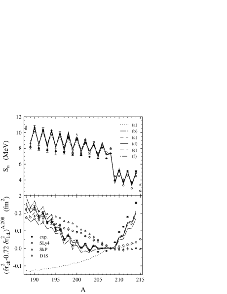
Figure 3: Upper panel: neutron separation energies $S_{\rm n}$ for lead isotopes. Lower panel: differences of mean squared charge radii $\delta\langle r^{2}\rangle_{\rm ch}$ with respect to ²⁰⁸Pb as reference nucleus; 72% of the corresponding liquid drop values (using $r_{0}=1.1$ fm) are subtracted to enhance the visibility of the small differences. Curves (a)–(f) correspond to the parameter sets (a)–(f) of the pairing force (15), respectively. Experimental data for $S_{\rm n}$ are from Ref.¹⁶, for $\delta\langle r^{2}\rangle_{\rm ch}$ from Refs.^26-28. For comparison, the HFB calculations with Skyrme forces SkP and SLy4, and with the Gogny D1S force but for even isotopes and ²¹¹Pb only, are also shown.

The results for the lead chain obtained with the elaborated coordinate-space technique and with the LEDF parametrization DF3 from Ref.[25] are shown in Fig. 3. The following parameter sets of the pairing force (6) are deduced (for the energy cutoff $\epsilon_{\rm c}=40$ MeV and the exponent $q=2/3$):

$$\begin{array}[]{lllllllr}f^{\xi}_{\rm ex}=-0.56,&h^{\xi}=0,&f^{\xi}_{\nabla}=0&\;(a);&\;f^{\xi}_{\rm ex}=-1.20,&h^{\xi}=0.56,&f^{\xi}_{\nabla}=2.4&\;(b);\\ f^{\xi}_{\rm ex}=-1.60,&h^{\xi}=1.10,&f^{\xi}_{\nabla}=2.0&\;(c);&\;f^{\xi}_{\rm ex}=-1.79,&h^{\xi}=1.36,&f^{\xi}_{\nabla}=2.0&\;(d);\\ f^{\xi}_{\rm ex}=-2.00,&h^{\xi}=1.62,&f^{\xi}_{\nabla}=2.0&\;(e);&\;f^{\xi}_{\rm ex}=-2.40,&h^{\xi}=2.16,&f^{\xi}_{\nabla}=2.0&\;(f).\\ \end{array}\,$$ (15)

As seen in the upper panel of Fig. 3, the neutron separation energies $S_{\rm n}$ are reproduced equally well for all parameter sets (a)–(f) of Eq. (15). The HFB calculations with two state-of-the-art Skyrme functionals SkP (Ref.[18]) and SLy4 (Ref.[29]) describe the $S_{\rm n}$ values with more or less the same quality as our curves (a)–(f), some deviations are observed above ²⁰⁷Pb. In the lower panel the calculated isotope shifts of mean squared charge radii, $\delta\langle r^{2}\rangle_{\rm ch}$, with respect to ²⁰⁸Pb as a reference nucleus are presented. Our curves except (a) do not differ from each other significantly and all of them reproduce qualitatively the kink and the size of odd-even staggering. The curve (a) corresponds to a simple contact pairing force which does not depend on density; in this case the behavior of $\delta\langle r^{2}\rangle_{\rm ch}$ is rather smooth and neither kink nor staggering are reproduced. One can see also that the Skyrme functionals SkP and SLy4 give too small kink and too small staggering. The Gogny D1S force could not reproduce the kink either. This fact clearly demonstrates the importance of including odd-mass nuclei in the fitting procedure of the force constants.

5 Ground-state properties of nuclear matter

Now, the empirical information gained from finite laboratory nuclei can be used to study the ground state properties and behavior of $\Delta$ as a function of density $\rho=2\rho_{0}x$ (or the Fermi momentum $k_{\rm F}=(3\pi^{2}\rho/2)^{1/3}=k_{0\rm F}x^{1/3}$) in infinite nuclear matter. Since the density-gradient term $\propto\!f^{\xi}_{\nabla}$ vanishes in this case, only two parameters are relevant: $f^{\xi}_{\rm ex}$ and $h^{\xi}$. The gap equation (11) reduces to

$$\Delta(x)=-\int\nolimits_{k\leq k_{\rm c}}\,\frac{d\vec{k}}{(2\pi)^{3}}{\cal F}^{\xi}(x)\frac{\Delta(x)}{2\sqrt{(\epsilon_{k}-\epsilon_{\rm F}(x))^{2}+\Delta^{2}(x)}}\,,$$ (16)

where $k_{\rm c}=\sqrt{2m(\epsilon_{\rm F}+\epsilon_{\rm c})}/\hbar$ and $\epsilon_{k}=\hbar^{2}k^{2}/2m$. Its solution in the weak pairing regime can be written as[30]:

$$\Delta(k_{\rm F})=c\epsilon_{\rm F}\exp\left[-\frac{\pi}{2}\cot\delta(k_{\rm F})\right]\,,$$ (17)

where $c=8{\rm e}^{-2}\approx 1.083$ and where we have introduced the Fermi level phase shift $\delta(k_{\rm F})$ defined by

$$k_{\rm F}\cot\delta(k_{\rm F})=-\frac{4k_{0\rm F}}{\pi}\left(\frac{1}{f^{\xi}(k_{\rm F})}+\frac{k_{\rm c}(k_{\rm F})}{2k_{0{\rm F}}}\right)-\frac{k_{\rm F}}{\pi}\ln\left(\frac{k_{\rm c}(k_{\rm F})-k_{\rm F}}{k_{\rm c}(k_{\rm F})+k_{\rm F}}\right)\,,$$ (18)

with $k_{\rm c}(k_{\rm F})=\sqrt{k_{0c}^{2}+k_{\rm F}^{2}}$; $k_{0c}=\sqrt{2m\epsilon_{\rm c}}/\hbar$. Eq. (18) corresponds to an exact solution of the nn scattering problem at the relative momentum $k=k_{\rm F}$ with the states truncated by a momentum cutoff $k_{\rm c}=k_{\rm c}(k_{\rm F})$ for contact potential $C_{0}f^{\xi}(k_{\rm F})\delta({\vec{r}})$ (see, e.g., Ref.[31]).

Shown in Fig. 4 are the results for $\Delta$ in nuclear matter with parameter sets of Eq. (15). Interestingly, for the sets (b)–(e), which reproduce satisfactorily both the $S_{\rm n}$ and $\delta\langle r^{2}\rangle_{\rm ch}$ values, there exists a “pivoting” point at $k_{\rm F}\approx 1.15$ fm^-1 (at $\approx$0.65 of the equilibrium density) with the same value of $\Delta_{\rm piv}\approx 3.3$ MeV. The approximation (17) (dashed curves in Fig. 4) works well in the entire range of $k_{\rm F}$ for the set (a), but for the other sets this is true only at $k_{\rm F}$ greater than $\approx$1.2 fm^-1 and also, for the sets (b), (c) and (d), at $k_{\rm F}$ less than 0.42, 0.14 and 0.042 fm^-1, respectively (in these regions, $\Delta/\epsilon_{\rm F}\leq 0.1$). It should be stressed that $\epsilon_{\rm F}$ entering the integrand of Eq. (16) can be expressed directly through density $\rho$ by $\epsilon_{\rm F}=\hbar^{2}k_{\rm F}^{2}(\rho)/2m$ with $k_{\rm F}(\rho)=(3\pi^{2}\rho/2)^{1/3}$ only if the pairing is weak and the dependence of the Fermi energy $\epsilon_{\rm F}$ (and the chemical potential $\mu$) on $\Delta$ can be disregarded. Otherwise one should introduce the particle number condition

$$x=\frac{2}{\rho_{0}}\int\nolimits_{k\leq k_{\rm c}}\,\frac{d\vec{k}}{(2\pi)^{3}}n_{k}(x),\quad n_{k}(x)=\frac{1}{2}\left(1-\frac{\epsilon_{k}-\epsilon_{\rm F}(x)}{\sqrt{(\epsilon_{k}-\epsilon_{\rm F}(x))^{2}+\Delta^{2}(x)}}\right)\,,$$ (19)

and to solve the system of the two equations (16) and (19) with respect to $\Delta$ and $\epsilon_{\rm F}$. The results shown in Fig. 4 by the solid curves correspond to such a solution.

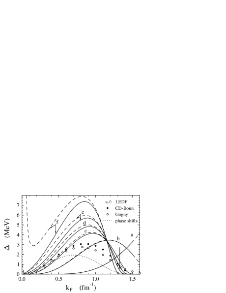
Figure 4: Pairing gap in nuclear matter as a function of the Fermi momentum. Full (dashed) curves (a)–(f) are obtained by solving Eqs. (16) and (19) (by using the weak pairing approximation of Eqs. (17) and (18)) with contact pairing force (6) and energy cutoff $\epsilon_{\rm c}=40$ MeV, and correspond, respectively, to the parameter sets (a)–(f) of Eq. (15). The vertical arrow marks the Fermi momentum at saturation point for the functional DF3 without pairing, $k_{0\rm F}=1.328$ fm^-1. The solid (open) circles are the solutions of the nonlocal gap equation with the CD-Bonn potential³² (with the finite-range Gogny D1 force³³). The dotted line is obtained from Eq. (17) with the free NN scattering phase shifts (see text).

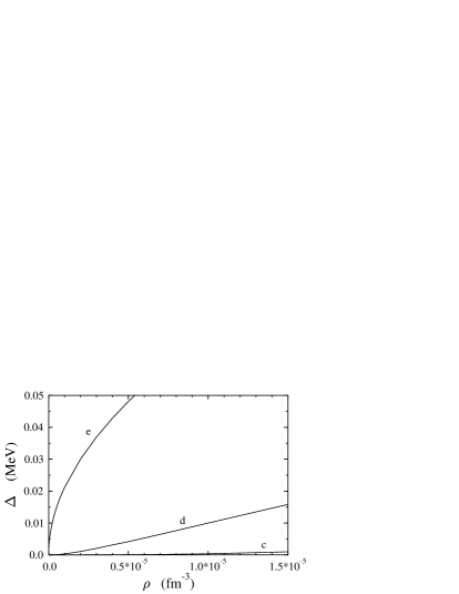
Figure 5: Pairing gap $\Delta$ as a function of $\rho$ at very low densities. Curves (c)–(e) correspond to the parameter sets (c)–(e) of Eq. (15), respectively.

All parameter sets (15) except (a) reproduce the neutron separation energies and the isotope shifts of charge radii $\langle r^{2}\rangle_{\rm ch}$ of lead isotopes fairly well (see Fig. 3). Shown also in Fig. 4 are the values of the ${}^{1}S_{0}$ pairing gap in nuclear matter obtained for the CD-Bonn potential[32] and for the Gogny D1 force[33]. The agreement between the two latter calculations is relatively good, while both deviate noticeably from our predictions. The curve for density-independent force, set (a), stands by itself with a positive derivative $d\Delta(x)/dx$ everywhere; no acceptable description of $\langle r^{2}\rangle_{\rm ch}$ could be obtained in this case[20].

At very low densities (18) reduces to

$$k_{\rm F}\cot\delta(k_{\rm F})\approx-\frac{1}{a_{\rm nn}}+\frac{1}{2}r_{\rm nn}k_{\rm F}^{2}-\frac{2k_{\rm F}}{\pi}\left[\frac{k_{\rm F}}{2k_{0c}}-\frac{2h^{\xi}}{(f^{\xi}_{\rm ex})^{2}}\left(\frac{k_{\rm F}}{k_{0\rm F}}\right)^{3q-1}\right]\,,$$ (20)

where $a_{\rm nn}$ is the singlet scattering length,

$$a_{\rm nn}=\frac{\pi}{2k_{0\rm F}}\left(\frac{\sqrt{2m\epsilon_{\rm c}}}{\hbar k_{0\rm F}}+\frac{2}{f^{\xi}_{\rm ex}}\right)^{-1}\equiv\frac{\pi}{4k_{0\rm F}}\left(\frac{1}{f^{\xi}_{\rm ex}}-\frac{1}{f^{\xi}_{\rm cr}}\right)^{-1}\,,$$ (21)

and $r_{\rm nn}$ is the effective range, $r_{\rm nn}=4/\pi k_{0c}$. Here we have introduced the critical constant $f^{\xi}_{\rm cr}=-2k_{0\rm F}/k_{0c}$, the vacuum strength $f^{\xi}_{\rm ex}$ at which the two-nucleon problem has a bound state solution at zero energy (in our case, $f^{\xi}_{\rm cr}=-1.912$).

The first two terms in (20) would describe the $s$-wave phase shift at low energies through an expansion of $k\cot\delta$ in powers of the relative momentum $k=k_{\rm F}$ if the interaction were density-independent – i.e., if the coupling strength and momentum cutoff were fixed by $f^{\xi}=f^{\xi}_{\rm ex}$ and $k_{\rm c}=k_{0c}$, respectively. It follows that, with a density-dependent effective force, such an expansion contains additional terms which are, for the parametrization used here, of the same order as the effective range term. This simply demonstrates that, for reproducing the pairing gap, the effective interaction even at very low densities need not necessarily coincide with the bare NN interaction as was discussed by Migdal many years ago[34].

At very low densities, at $k_{\rm F}\rightarrow 0$, to leading order from (18) we obtain

$$\Delta=c\epsilon_{\rm F}\exp{\left(\frac{\pi}{2k_{\rm F}a_{\rm nn}}\right)}\,,\quad a_{\rm nn}<0\,.$$ (22)

This expression agrees with the results of Ref.[35] based on a general analysis of the gap equation at low densities when $k_{\rm F}|a_{\rm nn}|\ll 1$.

But we should stress that (22) is valid only in the weak-coupling regime corresponding to negative $a_{\rm nn}$. In the opposite case, the gap in the dilute limit has to be found in a different way. At $f^{\xi}_{\rm ex}>f^{\xi}_{\rm cr}$, from (22) and (17) it follows that at low densities the pairing gap is exponentially small and eventually $\Delta(k_{\rm F}\rightarrow 0)=0$. Such a weak pairing regime with Cooper pairs forming in a spin singlet $l=0$ state exists up to the critical point at which the attraction becomes strong enough to change the sign of the scattering length. Then the strong pairing regime sets in, and $\Delta$ should be determined directly from the combined solution of Eqs. (16) and (19). In the dilute systems, $\epsilon_{\rm F}$ plays the role of the chemical potential $\mu$. At the critical point, $\mu$ becomes negative, and a bound state of a single pair of nucleons with the binding energy $\epsilon_{b}=2\mu$ ($=-\hbar^{2}/ma^{2}_{\rm nn}$) becomes possible[37]. In this regime, $\Delta$ can be found from (19). In the leading order we get

$$\Delta=\frac{\hbar^{2}}{m}\left(\frac{2\pi\rho}{a_{\rm nn}}\right)^{1/2}\,,\quad a_{\rm nn}>0\,.$$ (23)

It follows that, in the dilute case, the energy needed to break a condensed pair goes smoothly from $2\Delta$ to $2\mu=\epsilon_{b}$ as a function of the coupling strength as the regime changes from weak to strong pairing. But as seen from (22) and (23), the behavior of $\Delta$ is such that the derivative $d\Delta/d\rho$ at $\rho\rightarrow 0$ as a function of $f^{\xi}_{\rm ex}$ exhibits a discontinuity from 0 to $\infty$. This is illustrated in Fig. 5 where we have plotted $\Delta(\rho)$ for the sets (c)–(e) of Eq. (15), which embrace both regimes. Notice also that both analytical expressions (22) and (23) give a pure imaginary gap at the critical point, where the scattering length changes sign. When the Fermi momentum $k_{\rm F}$ approaches from below the upper critical point, where the pairing gap closes, $\Delta$ becomes exponentially small[35]. In weak coupling, $\Delta$ is also exponentially small at low densities. It is noteworthy that, as follows from (17), in both these cases the gap closes exactly at the points where the phase shift passes zero. As an illustration, we show in Fig. 4 by the dotted line the values of $\Delta(k_{\rm F})$ obtained from (17) using the “experimental” nn phase shifts. It is seen that $\Delta$ obtained this way closely follows the solution of the gap equation with the CD-Bonn potential[32] at low densities. The nn phase shift passes zero at the relative momentum $k=1.71$ fm^-1, and the gap should vanish at the corresponding Fermi momentum. Unfortunately, the solutions for $\Delta$ are given in Ref.[32] only in the region up to $k_{\rm F}=1.4$ fm^-1.

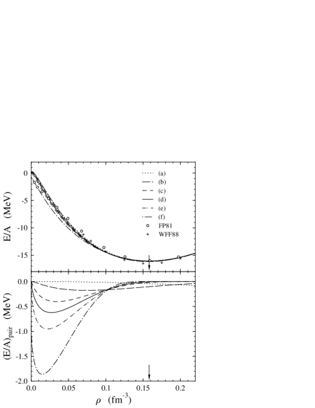
Figure 6: Energy per nucleon $E/A$ (top) and pairing contribution to $E/A$ (bottom) in nuclear matter. Curves (a)–(e) are calculated using Eq. (24) and correspond to the strength parameters (a)–(e) of Eq. (15), respectively. Open circles and stars are the calculations of Ref.¹⁰ and Ref.¹¹, respectively, for the UV14 plus TNI model. The vertical arrows mark the saturation density for the functional DF3 without pairing, $2\rho_{0}=0.1582$ fm^-3.

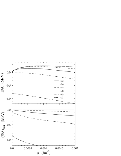
Figure 7: Energy per nucleon $E/A$ (top) and pairing contribution to $E/A$ (bottom) for nuclear matter at low densities. The notations are the same as in Fig. 6.

For nuclear matter, with our LEDF, the energy per particle is

$$\frac{E}{A}(x)=\frac{2}{\rho_{0}x}\int\nolimits_{k\leq k_{\rm c}}\frac{d\vec{k}}{(2\pi)^{3}}\frac{\hbar^{2}k^{2}}{2m}n_{k}(x)+\frac{1}{3}\epsilon_{0\rm F}a_{+}^{\rm v}f_{+}^{\rm v}(x)x+\frac{3\Delta^{2}(x)}{2f^{\xi}(x)x\epsilon_{0\rm F}}\,,$$ (24)

where $f_{+}^{\rm v}(x)=(1-h^{\rm v}_{1+}x)/(1+h^{\rm v}_{2+}x)$. Numerically, $a_{+}^{\rm v}=-6.422$, $h^{\rm v}_{1+}=0.163$ and $h^{\rm v}_{2+}=0.724$ (Ref.[25]). In the dilute limit the “particle-hole” term $\propto\!f_{+}^{\rm v}$ vanishes linearly in density. The chemical potential is

$$\mu(x)=\epsilon_{\rm F}(x)+\frac{1}{3}\epsilon_{0\rm F}a_{+}^{\rm v}[f^{{\rm v}\prime}_{+}(x)x^{2}+2f^{\rm v}_{+}(x)x]+\frac{3f^{\xi\prime}(x)}{2f^{\xi 2}(x)}\frac{\Delta^{2}(x)}{\epsilon_{0\rm F}}\,,$$ (25)

where the prime denotes a derivative with respect to $x$, $\epsilon_{\rm F}(x)$ and $\Delta(x)$ are determined from (16) and (19). The two last terms in (25), even in strong pairing regime, vanish in the dilute limit at least as $x^{q}$ if $0<q<1$ or linearly in $x$ if $q\geq 1$. We see again that, in strong coupling, in the leading order $\mu=\epsilon_{\rm F}=\epsilon_{b}/2<0$. The calculated energy per nucleon as a function of the isoscalar density $\rho$ is shown in the upper panel in Fig. 6 together with the results of the nuclear matter calculations[10, 11]. It is seen that DF3 gives qualitatively reasonable description of the nuclear matter EOS and that pairing could contribute noticeably to the binding energy especially at lower densities. In the lower panel in Fig. 6 we have plotted the pairing energy per nucleon, $(E/A)_{\rm pair}$, obtained by subtracting from (24) the corresponding value of $E/A$ at $\Delta=0$. The pairing contribution increases, as expected, when $f^{\xi}_{\rm ex}$ becomes gradually more attractive, with a shift to lower densities. For the sets (e) and (f) the attraction is strong, $f^{\xi}_{\rm ex}<f^{\xi}_{\rm cr}$. In these cases a nonvanishing binding energy in the dilute limit is solely due to Bose-Einstein condensation of the bound pairs, the spin-zero bosons, when all the three quantities, $\mu$, $E/A$ and $(E/A)_{\rm pair}$, reach the same value $\epsilon_{b}/2=\hbar^{2}/2ma^{2}_{\rm nn}$ ($\epsilon_{b}=-0.0646$ and $-1.616$ MeV for the set (e) and (f), respectively). This is illustrated in Fig. 7 where we have plotted $E/A$ and $(E/A)_{\rm pair}$ as functions of $\rho$ at very low densities.

We have considered the properties of nuclear matter with s-wave pairing within the LEDF framework, including extrapolation to the dilute limit, with a few possible parameter sets of the pairing force deduced from finite nuclei. At low densities, in the case of symmetric $N=Z$ matter, the ${}^{3}S_{1}-^{3}D_{1}$ pairing could be more important since the n–p force is more attractive than in the p–p or n–n pairing channels. Thus, our approach, with the ${}^{1}S_{0}$ pairing only, would be more appropriate for an asymmetric $N\neq Z$ case and for pure neutron systems. From this point of view the best choice for the LEDF calculations seems to be the parameter set (d) of Eq. (15) since it gives the singlet scattering length $a_{\rm nn}\approx-17.2$ fm which corresponds to a virtual state at $\approx 140$ keV known experimentally. As seen in Fig. 4, for this choice the behaviour of $\Delta$ at low densities agrees well with the calculations based on realistic NN forces. At higher densities, however, our predictions for $\Delta$ with the set (d) go much higher reaching a maximum of $\approx 4.84$ MeV at $k_{\rm F}\approx 0.92$ fm^-1, while the calculations of Ref.[32] give a maximum of about 3 MeV at $k_{\rm F}\approx 0.82$ fm^-1. With a bare NN interaction, if one assumes charge independence and that $m_{\rm n}=m_{\rm p}$, the pairing gap would be, at a given $k_{\rm F}$, exactly the same both in symmetric nuclear matter and in neutron matter. As shown in Refs.[38, 39], if one includes medium effects in the effective pairing interaction, $\Delta$ in neutron matter would be reduced substantially, to values of the order of 1 MeV at the most. Whether such a mechanism works in the same direction for symmetric nuclear matter is still an open question. The force (6) was chosen to be dependent on the isoscalar density only, since we have analyzed the existing data on $S_{\rm n}$ and $\delta\langle r^{2}\rangle_{\rm ch}$ for finite nuclei with a relatively small asymmetry, $(N-Z)/A\leq 0.25$. An extrapolation to neutron matter with such a simple force would give a larger pairing gap than for nuclear matter. This suggests that some additional dependence on the isovector density $\rho_{\rm n}-\rho_{\rm p}$ might be present in the effective pairing interaction.

6 Staggering and kinks in nuclear multipole excitations

The staggering phenomenon observed in the behavior of charge radii plotted as a function of neutron number is a prominent odd-even effect which has been systematically measured and widely discussed. Similar effects are expected to exist for other quantities such as neutron and matter radii, centroid energies of multipole excitations (position of the giant resonances), etc.

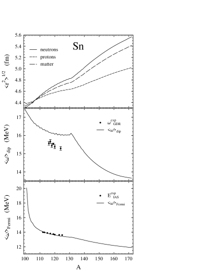
Figure 8: Neutron, proton and matter radii (top), mean energy of isovector dipole (middle) and Fermi charge-exchange (bottom) transitions for tin isotopes. The solid dots for $\bar{\omega}_{\rm dip}$ correspond to the experimental data for the maximum of the dipole photoabsorption Lorentz curves⁴⁴, while those for $\bar{\omega}_{F}$ to the experimental positions of the isobaric analog states with respect to the daughter nuclei⁴⁵.

Shown in the upper panel of Fig. 8 are the rms proton, neutron and matter radii for the tin isotopic chain calculated with the functional DF3 and with the set (d) of the pairing force. In the middle panel we show the mean energies $\bar{\omega}_{\rm dip}$ of dipole isovector excitations. These are calculated as the square root of the ratio $m_{3}/m_{1}$ with $m_{1}$ and $m_{3}$ the linear and cubic energy-weighted sum rule, i.e. the first and the third moment of the corresponding RPA strength distribution, respectively[40]:

$$\bar{\omega}_{\rm dip}=\left[-{{\hbar^{2}}\over{3m}}{A\over{NZ}}\int d\vec{r}d\vec{r}\,^{\prime}\,{{\partial\rho_{\rm n}}\over{\partial\vec{r}}}{\cal F}^{\rm np}(\vec{r},\vec{r}\,^{\prime}){{\partial\rho_{\rm p}}\over{\partial\vec{r}\,^{\prime}}}\right]^{1/2}\,.$$ (26)

Here ${\cal F}^{\rm np}$ is the effective neutron–proton interaction obtained from the energy-density functional as the second variational derivative $\delta^{2}E_{\rm int}/\delta\rho_{\rm n}\delta\rho_{\rm p}$. In the lower panel of Fig. 8 we show the mean energies $\bar{\omega}_{\rm F}$ of the charge-exchange $0^{+}$ excitations, i.e. the Fermi transitions, in tin nuclei with $N>Z$. These energies are calculated within the sum rule approach as the ratio $(m_{1}^{+}+m_{1}^{-})/(m_{0}^{+}-m_{0}^{-})$ with $m_{1}^{+}$ and $m_{1}^{-}$ the first moment of the strength distribution of the Fermi transitions in the $\beta^{+}$ and $\beta^{-}$ channel, respectively (energy-weighted sum rules) and with $m_{0}^{+}$ and $m_{0}^{-}$ the corresponding non-energy weighted sum rules. The expression for $\bar{\omega}_{\rm F}$ reads (see, e.g. Ref.[41]):

$$\bar{\omega}_{\rm F}={1\over{N-Z}}\int d\vec{r}\,U_{\rm Coul}(\vec{r}\,)\left(\rho_{\rm n}(\vec{r}\,)-\rho_{\rm p}(\vec{r}\,)\right)\,,$$ (27)

where $U_{\rm Coul}$ is the Coulomb mean field potential. It is seen in Fig. 8 that the neutron, proton and matter radii as functions of the mass number $A$ reveal a kink at magic ¹³²Sn, and at larger $A$ the difference between rms neutron and proton radii starts to increase more rapidly. The staggering in radii is observed mostly in the region between the two magic nuclei, from ¹⁰⁰Sn to ¹³²Sn, and this effect is practically washed out beyond $A=140$. The mean energy of dipole transitions occurs to be in anticorrelation with such a behavior in radii, and this seem to be in qualitative agreement with experimental data (one should mention that Eq. (26) overestimates the position of the giant dipole resonance by $\approx 0.5$ MeV because of the cubic energy-weighted sum rules used in the derivation of $\bar{\omega}_{\rm dip}$). One also observes a distinct kink in the behaviour of $\bar{\omega}_{\rm dip}$ at $A=132$. Beyond this magic number the mean dipole energy decreases rather fast and then nearly saturates when approaching $A=172$. This might be connected with an enhancement of the low-energy dipole transitions[42] and also with possible appearance of the so-called soft dipole mode[43] in nuclei near the neutron drip line. The anticorrelations in the staggering behavior of $\bar{\omega}_{\rm dip}$ and the rms radii $\langle r^{2}\rangle^{1/2}_{\rm n}$, $\langle r^{2}\rangle^{1/2}_{\rm p}$ can easily be understood by considering the influence of pairing on the gradients of neutron and proton densities entering Eq. (26). The odd-even effect in $\bar{\omega}_{\rm dip}$ is constructive and more pronounced in the $A\leq 132$ region where both gradients strongly overlap. Beyond $A=132$ the larger differences between neutron and proton rms radii imply a lower overlap between neutron and proton density gradients at the nuclear surface, hence a smaller mean dipole energy. The situation with mean energy of the Fermi charge-exchange transitions is different. From Eq. (27) one expects that the correlation between $\bar{\omega}_{F}$ and the neutron and proton rms radii should be destructive. As seen in the lower panel in Fig. 8, the staggering in the evolution of $\bar{\omega}_{F}$ with $A$ is very weak indeed and almost invisible. The kink at the magic mass number $A=132$ is also much less pronounced compared to the dipole case. Remarkable enough, the theoretical self-consistent sum-rule predictions for $\bar{\omega}_{F}$ in tin isotopes are in excellent agreement with the available experimental data on the position of the isobaric analog states.

References

- [1] R.B. Wiringa, Nucl. Phys. A 631, 70c (1998).
- [2] A. Akmal et al., Phys. Rev. C 58, 1804 (1998).
- [3] M. Baldo, I. Bombachi and C.F. Burgio, Astron. Astrophys. 328, 274 (1997).
- [4] K. Pomorski et al., Nucl. Phys. A 624, 349 (1997).
- [5] Z. Patyk et al., Phys. Rev. C 59, 704 (1999).
- [6] P. Möller et al., ADNDT 59, 185 (1995).
- [7] Y. Aboussir et al., ADNDT 61, 127 (1995).
- [8] S.A. Fayans, JETP Lett. 68, 169 (1998).
- [9] A.V. Smirnov et al., Sov. J. Nucl. Phys. 48, 995 (1988).
- [10] B. Friedman and V.R. Pandharipande, Nucl. Phys. A 361, 502 (1981).
- [11] R.B. Wiringa, V. Fiks and A. Fabrocini, Phys. Rev. C 38, 1010 (1988).
- [12] V.A. Khodel and E.E. Saperstein, Phys. Reports 92, 183 (1982).
- [13] A. Bulgac and V.R. Shaginyan, Nucl. Phys. A 601, 103 (1996).
- [14] S.A. Fayans and D. Zawischa, Phys. Lett. B 383, 19 (1996).
- [15] G.A. Lalazissis, S. Raman and P. Ring, ADNDT 71, 1 (1999).
- [16] G. Audi and A.H. Wapstra, Nucl. Phys. A 565, 66 (1993).
- [17] A. Bulgac, Preprint FT-194-1980, Bucharest, 1980; nucl-th/9907088.
- [18] J. Dobaczewski, H. Flocard and J. Treiner, Nucl. Phys. A 422, 103 (1984).
- [19] S.T. Belyaev et al., Sov. J. Nucl. Phys. 45, 783 (1987).
- [20] S.A. Fayans et al., JETP Lett. 68, 276 (1998); Nuovo Cim. 111 A, 823 (1998).
- [21] P. Ring and P. Schuck, The nuclear many-body problem (Springer, NY, 1980).
- [22] S.A. Fayans et al., submitted to Nucl. Phys. A.
- [23] D. Zawischa, U. Regge and R. Stapel, Phys. Lett. B 185, 299 (1987).
- [24] S.A. Fayans et al., Phys. Lett. B 338, 1 (1994).
- [25] I.N. Borzov et al., Z. Phys. A 355, 117 (1996).
- [26] M. Anselment et al., Nucl. Phys. A 451, 471 (1986).
- [27] E.W. Otten, in Treatise on Heavy Ion Science, ed. D.A. Bromley (Plenum Press, NY, 1989), Vol. 8, p. 515.
- [28] S.B. Dutta et al., Z. Phys. A 341, 39 (1991).
- [29] E. Chabanat, Interactions effectives pour des conditions extrêmes d’isospin, Université Claude Bernard Lyon-1, Thesis 1995, LYCEN T 9501, unpublished.
- [30] S.A. Fayans, JETP Lett. 70, 240 (1999).
- [31] H. Esbensen, G.F. Bertsch and K. Hencken, Phys. Rev. C 56, 3054 (1997).
- [32] Ø. Elgarøy and M. Hjorth-Jensen, Phys. Rev. C 57 1174 (1998).
- [33] H. Kucharek et al., Phys. Lett. B 216 249 (1989).
- [34] A.B. Migdal, Theory of Finite Fermi Systems and Applications to Atomic Nuclei (Interscience, NY, 1967).
- [35] V.A. Khodel, V.V. Khodel and J.W. Clark, Nucl. Phys. A 598, 390 (1996).
- [36] L.P. Gor’kov and T.K. Melik-Barkhudarov, Sov. Phys. JETP 13, 1018 (1961).
- [37] P. Nozières and S. Schmitt-Rink, J. Low Temp. Phys. 59, 195 (1985).
- [38] J. Wambach, T.L. Ainsworth and D. Pines, Nucl. Phys. A 555,128 (1993).
- [39] H.-J. Schulze et al., Phys. Lett. B 375 1 (1996).
- [40] S.V. Tolokonnikov and S.A. Fayans, JETP Lett. 35, 403 (1982).
- [41] N.I. Pyatov and S.A. Fayans, Sov. J. Part. Nucl. 14, 401 (1983).
- [42] I. Hamamoto, H. Sagawa and X.Z. Zhang, Phys. Rev. C 53, 765 (1996).
- [43] S.A. Fayans, Phys. Lett. B 267, 443 (1991).
- [44] A. Leprêtre et al., Nucl. Phys. A 219 39 (1974).
- [45] Evaluated Nuclear Structure Data File, http://www.nndc.bnl.gov/nndc/ensdf.