Pairing-induced localization of the particle
continuum in weakly bound nuclei

Abstract

The Hartree-Fock-Bogolyubov (HFB) problem for the cutoff local energy-density functional is solved numerically by using the Gor’kov formalism with an exact treatment of the particle continuum. The contributions from the resonant and “gas” continuum to the spectral density of the HFB eigenstates as well as the shifting and broadening of the discrete HF hole orbitals are clearly demonstrated with the illustrative example of the drip-line nucleus ⁷⁰Ca. The structure of the neutron density distribution in the localized ground state is analyzed, and the formation of its extended tail (“halo”) is shown to be a collective pairing effect.

PACS: 21.60.-n; 21.90.+f; 24.10.Cn

Keywords: Local energy-density functional; pairing correlations; localized states in the continuum; drip-line nuclei; neutron halo

, ,

Pairing correlations significantly influence the properties of finite nuclei producing, e.g., the observed odd-even staggering of the binding energies and radii. In the mean-field models, the pairing is introduced either at the BCS or the HFB level [1]. The zone of the active phase space around the Fermi surface, in which the major pairing effects are developed, depends on the effective interaction used. Whenever this zone includes states from the particle continuum, and this is obviously inevitable when approaching the drip line, the BCS approximation breaks down, yielding unphysical nucleonic gas [2]. A correct treatment of the pairing problem with continuum is provided by the HFB theory which, for the chemical potential $\mu<0$, always gives a localized ground state [3]. In principle, an exact solution of the HFB equations should be found with the physical boundary conditions both for the bound and scattering states (examples of such solutions are given in [4, 5]). However, in most applications of the HFB theory to nuclei, with different kinds of the energy-density functionals, the particle continuum is discretized in a box (see, e.g., [6, 7] and references therein), and it is still questionable whether or not the particle level density can be well reproduced with such a prescription, particularly near the threshold. Continuum effects have been studied very recently in [8] within the HFB method using a fixed, analytically soluble mean field potential and keeping self-consistency only in the pairing channel; again, the continuum states have been discretized in a spatial box. An attempt to take into account the resonant continuum within the HF+BCS approach has been also made recently in [9, 10]. One should notice that, for a nucleus with even $N$ (we consider the neutron subsystem for definiteness), all HFB solutions with energies $E>|\mu|\approx S_{2\rm n}/2$ ($S_{2\rm n}$ is the two-neutron separation energy) belong to the continuum, and these solutions contain both localized and non-localized HFB resonances. Their positions and widths, as well as the genetic relation to the Hartree-Fock (HF) single-particle spectrum, and also the contribution from the nonresonant continuum are worth to be revealed with numerically “exact” HFB calculations. Of particular interest is the situation on the drip line where the nuclei have only one bound state — the ground state, and the whole HFB spectrum is continuous. Our study is motivated by the great activity in physics of radioactive nuclear beams which have lead already, e.g., to the discovery of halo structure in some loosely bound nuclei.

Our approach is based on the generalized variational principle applied to the cutoff (local) energy-density functional [11, 12, 13] and on the physically transparent and mathematically elegant Green’s function method. The coordinate-space technique used to solve the Gor’kov equations exactly, for spherical systems with a local pairing field, is described in detail in [4, 11, 13]. Here we shall discuss the results for Ca isotopes obtained with functional DF3 whose normal part is parametrized in Ref. [14]. In the anomalous (pairing) part we employ the contact “gradient” pairing force [15] with a density-dependent form factor

$${\mathcal{F}}^{\xi}=1.35\times C_{0}\left(f^{\xi}_{\rm ex}+h^{\xi}x^{2/3}(\vec{r})+f^{\xi}_{\nabla}r_{0}^{2}\left({\vec{\nabla}}x(\vec{r})\right)^{2}\right)\,,$$ (1)

where $x=(\rho_{\rm n}+\rho_{\rm p})/2\rho_{0}$ is the isoscalar dimensionless density with $\rho_{\rm n(p)}$ the neutron (proton) density and $\rho_{0}$ the equilibrium density of one kind of particles in symmetric nuclear matter with the Fermi energy $\epsilon_{0\rm F}$; $C_{0}=2\epsilon_{0\rm F}/3\rho_{0}$ is the inverse density of states at $\epsilon=\epsilon_{0\rm F}$; $r^{2}_{0}=(3/8\pi\rho_{0})^{2/3}$ (for DF3, $C_{0}=308.2$ MeV$\cdot$fm³ and $r_{0}=1.147$ fm). The pairing strength parameters $f^{\xi}_{\rm ex}=-1.79$, $h^{\xi}=1.36$ and $f^{\xi}_{\nabla}=2.0$ have been deduced from the neutron separation energies and charge radii in the Pb isotope chain [13], both the staggering and kink being well reproduced. As shown in Ref. [13], the force (1) with the scaling factor of 1.35 allows to nicely reproduce the analogous differential observables in the Ca isotopes including the anomalous behavior of charge radii. All calculations are done with a fixed energy cutoff of 40 MeV above the Fermi level in any given nucleus.

The HFB problem with the above energy-density functional is solved iteratively by using the coordinate-space technique in the complex energy plane. The normal and anomalous densities at each iteration are evaluated as the contour integrals of the generalized Green’s function $\hat{G}$ which obey the Gor’kov equation $(E-\hat{\mathcal{H}})\hat{G}(E)=\hat{I}$ with $\hat{\mathcal{H}}$ the HFB Hamiltonian. For spherical systems, after separating the spin-angular variables one gets the equation for the radial component $\hat{g}_{jl}$ of the generalized Green’s function $\hat{G}$:

$$\left(\begin{array}[]{cc}E-h_{jl}+\mu&-\Delta\\ -\Delta&E+h_{jl}-\mu\end{array}\right)\left(\begin{array}[]{cc}g^{11}_{jl}&\;g^{12}_{jl}\\ g^{21}_{jl}&\;g^{22}_{jl}\end{array}\right)(r,r^{\prime};E)=\left(\begin{array}[]{cc}\delta(r-r^{\prime})&0\\ 0&\delta(r-r^{\prime})\end{array}\right)\,,$$ (2)

where $h_{jl}=\textstyle{\frac{\hbar^{2}}{2m}}(-\textstyle{\frac{d^{2}}{dr^{2}}+\frac{l(l+1)}{r^{2}}})+U_{\rm c}(r)+U_{sl}(r)\langle\vec{\sigma}\vec{l}\rangle_{jl}$ is the Hartree-Fock (HF) Hamiltonian in the $jl$ channel with $U_{\rm c}$ and $U_{sl}$ the central and spin-orbit potentials, respectively; $\langle\vec{\sigma}\vec{l}\rangle_{jl}=j(j+1)-l(l+1)-\textstyle{\frac{3}{4}}$; $E\geq 0$. The solution of this matrix equation is constructed by using the four linearly independent solutions $(u_{i},v_{i}),i$=1–4, which satisfy the homogeneous system obtained from (2) by replacing the right hand side by zero [4, 13]. Two of them are regular at $r\rightarrow 0$ and the other two are regular at $r\rightarrow\infty$. The latter are chosen with the asymptotic momenta $k_{\pm}=\sqrt{\mu\pm E}$ such that ${\rm Im}k_{\pm}\geq 0$ which provides, in particular, the correct asymptotics for the particle scattering states at the ${\rm Im}E=0$ axis. Such boundary conditions ensure the spatial localization of the nuclear ground state at $\mu<0$ [3, 4].

It is convenient to study the pairing effects in terms of the spectral distributions over the eigenstates of the HFB Hamiltonian, i.e. in terms of the spatial integrals of the imaginary parts of the Gor’kov Green’s functions. Here, for the given $jl$ quantum numbers, we shall consider two partial spectral distributions:

$$\frac{\d N^{22}_{jl}}{\d E}=-\frac{2j+1}{\pi}\int_{0}^{R}{\rm Im}g^{22}_{jl}(r,r;E)\d r\,,$$ (3)

and

$$\frac{\d N^{11}_{jl}}{\d E}=-\frac{2j+1}{\pi}\int_{0}^{R}{\rm Im}g^{11}_{jl}(r,r;E)\d r\,.$$ (4)

The first and the second we shall call the $v^{2}$- and $u^{2}$-spectral density, respectively. The corresponding analytical expressions can be obtained by using the partial Green’s functions which incorporate the generalized Wronskian of the four linearly independent solutions as given in Refs. [4, 13]. We add that the expressions for the canonical-basis spectral distributions and the numerical results with discretized continuum for a few tin isotopes can be found in Ref. [6].

In eq. (3), the spatial integral converges for $R\rightarrow\infty$ since it includes only the localized components $\propto{v^{2}}$. At $E>|\mu|$, all HFB eigenstates are in the continuum and, since ${\rm Im}g^{11}_{jl}$ contains non-localized components $\propto{u^{2}}$, the integration in eq. (4) is meaningful only up to a certain finite range $R$. One may present the two above expressions by one function $\d N_{jl}^{\rm HFB}/\d\epsilon$ if (3) and (4) are considered as functions of $\epsilon=\mu-E$ and $\epsilon=\mu+E$, respectively, though both are for the same HFB eigenvalue $E$.

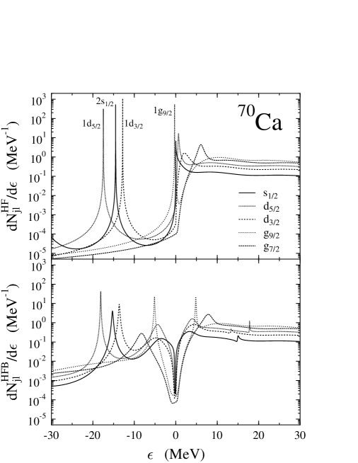
Figure 1: Neutron even-$l$ partial spectral densities in drip-line nucleus ⁷⁰Ca calculated by integrating the imaginary parts of the corresponding Green’s functions up to $R=10$ fm. A smearing parameter $\gamma=1$ keV is used to visualize the $\delta$-like peaks and very narrow resonances. Upper panel: level densities for the “HF” potential; the $\epsilon<0$ part for the discrete spectrum with indicated single-particle levels, the $\epsilon>0$ part for continuum states. Lower panel: the HFB results; all states are in the continuum, the left part ($\epsilon<0$) is for the localized $v^{2}$-spectral density, the right ($\epsilon>0$) for the non-normalizable $u^{2}$-components (see text).

Figure 2: The same as in Fig. 1 but for the odd-$l$ states.

We show in Figs. 1 and 2 the partial HFB neutron spectral densities for even and odd $l$, respectively, calculated for the drip-line nucleus ⁷⁰Ca, as functions of $\epsilon$ with $R$=10 fm (lower panels) and also present the corresponding “HF” level densities (upper panels). The “HF” refers to the results obtained by solving eq. (2) but keeping only the diagonal part of $\hat{\mathcal{H}}$ which emerges after solving the HFB problem ($h_{jl}$ includes the contribution from pairing correlations). In other words, in these figures we show the level densities for the basis which diagonalizes the mean field part of the HFB Hamiltonian versus the spectral densities which arise when the pairing field $\Delta$ is present explicitly in the left matrix in eq. (2). We point out that the spherical volume of radius $R$=10 fm is chosen here as the physical volume in which the mean-field and pairing correlations are mostly active to produce the localized ground state, it is not a normalization box; within this volume we integrate the imaginary parts of the Green’s functions which have the correct asymptotic behavior (the normal and anomalous densities, when solving the HFB problem, have been evaluated up to 25 fm, and, again, the wave functions are not zero at and beyond this radius, but the contribution from this far region to the bulk ground state properties is negligible). For the visualization of the $\delta$-like peaks associated with the discrete “HF” states and very narrow resonances, a small imaginary part $\gamma$=1 keV has been added to the energy $E$ in the Green’s functions. The obtained chemical potential is small, $\mu=-149$ keV; the spectral densities within the region $2\mu<\epsilon<0$ should vanish, and those which appear in Figs. 1 and 2 at these energies are due to the smearing parameter $\gamma$.

Let us discuss first the peculiarities in the “HF” level densities. For a finite-depth potential well, such as our neutron HF potential, it can be shown that the partial single particle level density in the continuum within a spherical volume with radius $R$ larger than the potential range is given by

$$\frac{\d N^{\rm HF}_{jl}}{\d\epsilon}=\frac{2j+1}{\pi}\left\{\frac{\d\delta_{jl}}{\d\epsilon}+\frac{k^{3}R^{3}}{2\epsilon}\left[\left(Y^{l}_{jl}(kR)\right)^{2}-Y^{l-1}_{jl}(kR)Y^{l+1}_{jl}(kR)\right]\right\}\,,$$ (5)

where $Y^{i}_{jl}(kR)=(\cos\delta_{jl})j_{i}(kR)-(\sin\delta_{jl})n_{i}(kR),\,i=l,l\pm 1;\,k=\sqrt{2m\epsilon}/\hbar$. This formula is valid for $R$ big enough so that the radial wave function can be expressed through spherical Bessel and Neumann functions ($j_{l}$ and $n_{l}$, respectively) and the phase shift $\delta_{jl}(\epsilon)$ can be calculated accurately. The resonance-like bumps seen in the upper panels in Figs. 1 and 2 at $\epsilon>0$ are associated with the term $\d\delta_{jl}/\!\d\epsilon$ in (5). These bumps are imposed on a rather flat nonresonant continuum which weakly oscillates with an energy-dependent wavelength defined by $\Delta(kR)\approx 2\pi$. Without potential, when $\delta_{jl}(\epsilon)\equiv 0$, eq. (5) gives the free-gas partial level density. Subtracting the latter from eq. (5), at $kR\gg l$ one gets

$$\frac{\d N^{\rm HF}_{jl}}{\d\epsilon}-\frac{\d N^{\rm gas}_{jl}}{\d\epsilon}=\frac{2j+1}{\pi}\left[\frac{\d\delta_{jl}}{\d\epsilon}-\cos(2kR+\delta_{lj})\frac{\sin\delta_{lj}}{2\epsilon}\right]\,.$$ (6)

Averaging this expression over small energy range $\Delta\epsilon>\pi\sqrt{2\hbar^{2}\epsilon/mR^{2}}$ eliminates the oscillating cosine term, and one is left with the usual level density $\propto\d\delta_{jl}/\!\d\epsilon$ associated with the potential well itself (see also Ref. [16]). However, this procedure can not be applied at low energies, i.e. in the region near the continuum threshold which, in drip-line nuclei, is very close to the Fermi surface. This zone of the phase space is of importance since the major pairing effects are developed around the Fermi surface. At any finite $R$, when $\epsilon\rightarrow 0$, the leading term $\propto k^{2l-1}$ of the expansion of $\d\delta_{jl}/\!\d\epsilon$ in powers of $k$ cancels in eq. (5) due to the contribution coming from the term $\propto\sin(2\delta_{jl})j_{l-1}(kR)n_{l+1}(kR)$. The resulting level density near the continuum threshold turns out to be proportional to $C_{jl}k^{2l+1}$, i.e. it has the free-gas behavior, the coefficients $C_{jl}$ depend, however, on the potential well. For the $s$-wave level density, using the effective range approximation, we get from (5) and (6) an analytical expression:

$$\frac{\d N^{\rm HF}_{\frac{1}{2}0}}{\d\epsilon}=\frac{2}{3\pi}\frac{k^{3}}{\epsilon}R^{3}\left\{1-3\frac{a}{R}\left[1-\frac{a}{R}\left(1-\frac{1}{2}\frac{r_{\rm eff}}{R}\right)\right]\right\}\,.$$ (7)

where $a$ is the scattering length and $r_{\rm eff}$ is the effective range. In the curly brackets here is a factor which could give an enhancement of the HF level density as compared to the free-gas one. For our “HF” potential we found $a=-14.8$ fm and $r_{\rm eff}=14.4$ fm, which gives, with $R=10$ fm, an enhancement factor of about 7. These parameters correspond to the virtual $s$-state at $\epsilon_{0}=-51$ keV which shows up as a sharp peak at very low positive $\epsilon$ in the upper panel in Fig. 1. The width of this very asymmetric peak at half maximum is about 23 keV. At larger energies, one can see in this panel two partners of the $d$-wave resonance which is split due to the spin-orbit potential, and also the $g_{7/2}$ resonance whose $g_{9/2}$ partner is in the discrete spectrum at $\epsilon=-276$ keV. Besides, a negative-parity $h_{11/2}$ resonance can be seen in the upper panel in Fig. 2. The resonance characteristics and the energies $\epsilon_{\lambda}^{0}$ of some bound “HF” states are listed in Table 1 (the first three columns).

Table 1.

Characteristics$\,{}^{a}$ of some “HF” states and localized

$v^{2}$-components of the HFB resonances in ⁷⁰Ca

state “HF” HFB $$\lambda \epsilon^{0}_{\lambda} \Gamma^{0}_{\lambda} \epsilon_{\lambda} \Gamma_{\lambda} - \,{}^{b} \approx 0.023\,^{b} - - - - - - - - - - - 5\times 10^{-5} - - - - - - - - - - - - 1\times 10^{-4} - -$$ 3s_1/2 0.051 3.467 4.574 2d_5/2 +0.659 0.192 4.369 2.150 2d_3/2 +2.097 2.038 4.859 4.483 1g_9/2 0.276 5.132 0.144 1f_5/2 2.666 5.559 0.115 2p_1/2 4.261 6.285 0.122 2p_3/2 6.193 7.621 1g_7/2 +6.064 1.419 8.236 2.115 1h_11/2 +8.106 0.915 9.896 1.330 1f_7/2 8.980 10.071 0.145 1d_3/2 12.814 13.663 0.277 2s_1/2 14.514 15.265 0.306 1d_5/2 17.467 18.103 0.086 1p_1/2 22.962 23.328 1p_3/2 25.564 25.894 0.003 ^a Energies and widths are in MeV. ^b Virtual state (see text).

The graphical presentation of Fig. 1 and 2 has the advantage that the HFB spectral densities from the lower panels would be smoothly transformed to the corresponding upper “HF” ones if the $\Delta$’s in the HFB Hamiltonian of eq. (2) could be smoothly switched off keeping the “HF” part $h_{jl}$ unchanged and defining $\mu$ by the particle number condition. In this way, one can easily trace the genetic origin of the irregularities seen in the HFB spectral densities. In particular, the resonance contributions from the particle continuum to the localized $v^{2}$-spectral density can be recognized. The characteristics of the picked-out localized $v^{2}$-parts of the HFB resonances are listed in Table 1 attributing them the genetic “HF” $jl$ quantum numbers (the fourth and fifth columns). The widths of the “HF” resonance states and of the localized $v^{2}$-components of the HFB resonances have been estimated from a 3-point no-background Breit-Wigner fit of the corresponding maxima. One can see that the discrete “HF” states get widths, i.e. they become the HFB resonances whose $v^{2}$-components are shifted, as expected, to lower $\epsilon$. The HFB nonresonant background can be also seen in the lower panels of Figs. 1 and 2. The non-localized $u^{2}$- and localized $v^{2}$-components of the HFB resonances are located symmetrically with respect to $\epsilon=\mu$ (i.e., $E=0$). We remark that all these belong to the same HFB eigenstate, however we do not discuss here the properties of the $u^{2}$-components due to lack of space.

As seen in Fig. 1, the $1g_{9/2}$ “HF” state at $\epsilon_{\lambda}^{0}=-276$ keV becomes, with pairing, a HFB resonance whose localized $v^{2}$-component lies well below the continuum threshold, at $\epsilon\approx-\bar{\Delta}$ where $\bar{\Delta}$ is the diagonal matrix element of the pairing field over the “HF” states near the Fermi surface. In our case, the energy gap $2\bar{\Delta}$ between the two components of this resonance is rather big, $\approx 10$ MeV. This could lead to the noticeable reduction of the tail of the neutron density distribution (the so-called pairing anti-halo effect [8, 7]). However, in the drip-line nuclei, when $|\mu|\ll\bar{\Delta}$, near the threshold there appear strong localized $v^{2}$-components from the resonant and non-resonant parts of the particle continuum with different $jl$. This is clearly seen in the lower panels of Figs. 1 and 2.

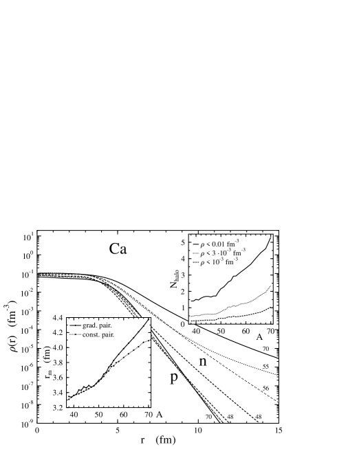
Figure 3: Neutron and proton densities for some Ca isotopes resulting from the spherical HFB calculations with functional DF3 and gradient pairing force of eq.(1). The curves are marked with the mass number $A$. The two inserts are both for even- and odd-$A$, up to the drip-line nuclei ⁷⁰Ca and ⁵⁵Ca, respectively. Right upper insert: the number of neutrons in the “halo” region where the density does not exceed the indicated values (0.01, 0.003 and 0.001 fm^-3). Left lower insert: the rms matter radii in comparison with “constant-pairing” HFB results (see text).

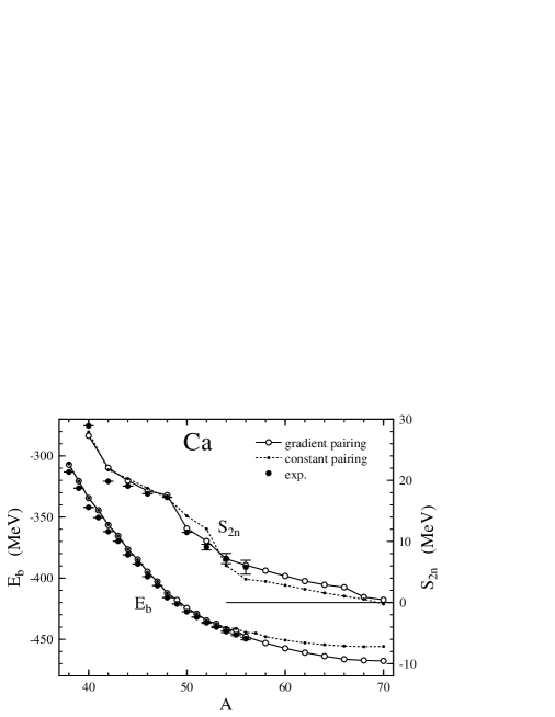
Figure 4: Binding energies $E_{\rm b}$ (lower curves, left scale) and two-neutron separation energies $S_{2{\rm n}}$ (upper curves, right scale) in even Ca isotopes. Solid (dashed) lines connect the points resulting from the spherical HFB calculations with functional DF3 and gradient (“constant”) pairing force (see text). Experimental data and those derived from systematics are from [17].

The “HF” and HFB partial neutron occupation numbers $N_{jl}$ in ⁷⁰Ca are listed in Table 2. Also given in this table are the numbers of neutrons $N_{jl}(r>R_{1})$ and $N_{jl}(r>R_{2})$ in the tail of $\rho_{\rm n}$ beyond the nuclear surface; $R_{1}$ and $R_{2}$ are defined by $\rho_{\rm n}(R_{1})=0.01$ fm^-3 and $\rho_{\rm n}(R_{2})=0.001$ fm^-3, respectively. The choice of $R_{1}$ roughly corresponds to the radius $R_{\rm F}+t/2$ where $t=4(\ln 3)d$ is the width of the diffuse zone approximated in the usual way by the Fermi function $\propto\{1+\exp[(r-R_{\rm F})/d]\}^{-1}$. The calculated densities for Ca isotopes with $A=38$ to 70 (a few of them are shown in Fig. 3) can be well described in the surface region by such a Fermi distribution. For ⁷⁰Ca, we found $R_{\rm F}=4.60$ fm and $d=0.73$ fm which gives $R_{1}=6.2$ fm (for comparison: in ⁴⁸Ca, $R_{\rm F}=3.85$ fm, $d=0.52$ fm and $R_{1}=5.0$ fm; thus, approaching the drip line, the size of the diffuse surface zone is significantly increasing). Using a larger radius $R_{2}$, one can characterize the $jl$ composition of the outmost tail of $\rho_{\rm n}$ in the “halo” region. Table 2 shows that the pairing makes the $N_{jl}$ distribution more “uniform” than in the “HF” case, the major effect is due to the depletion of the discrete “HF” orbitals $g_{9/2}$, $f_{7/2}$ and $f_{5/2}$ and filling the resonance structures from the “HF” continuum ($3s_{1/2}$, $2d_{5/2}$, etc., see Table 1). The partial neutron numbers in the “halo” region are also distributed more uniformly, the contributions from the states with higher angular momenta, up to $l=8$, are not negligible. Thus, in our calculations, the composition of the extended tail of the neutron density distribution in ⁷⁰Ca is determined by a collective pairing effect.

Table 2.

Partial neutron occupation numbers in ⁷⁰Ca

$$N_{jl} N_{jl}(r>R_{1})\,^{a} N_{jl}(r>R_{2})\,^{b} lj R_{1} R_{1} R_{2} R_{2} \Sigma_{lj}\, R_{1} \rho_{\rm n}(R_{1})=0.01 R_{2} \rho_{\rm n}(R_{2})=0.001$$ “HF” HFB “HF” HFB “HF” HFB =6.10 fm =6.15 fm =7.60 fm =8.15 fm s_1/2 4 4.740 0.079 0.501 0.007 0.176 p_3/2 8 7.861 0.612 0.711 0.120 0.146 p_1/2 4 3.774 0.408 0.393 0.104 0.083 d_5/2 6 8.207 0.094 0.920 0.006 0.204 d_3/2 4 4.725 0.088 0.439 0.008 0.103 f_7/2 8 8.012 0.362 0.554 0.039 0.077 f_5/2 6 4.599 0.589 0.503 0.129 0.073 g_9/2 10 5.274 1.267 0.633 0.294 0.072 g_7/2 0.877 0.211 0.035 h_11/2 0.925 0.191 0.026 h_9/2 0.292 0.097 0.018 i_13/2 0.321 0.087 0.014 i_11/2 0.136 0.059 0.011 j_15/2 0.144 0.052 0.009 j_13/2 0.054 0.035 0.008 k_17/2 0.040 0.026 0.006 k_15/2 0.019 0.016 0.005 : 50 50.00 3.500 5.429 0.707 1.067 ^a is defined by the condition  fm^{-3 b} is defined by the condition  fm^-3

The numbers of neutrons beyond the diffusive surface, $N_{\rm halo}$, calculated both for even and odd Ca isotopes with $A=38$ to 70 are shown in the right insert in Fig. 3. Depending on the choice of the upper limit for the tail density, 0.01, 0.003 or 0.001 fm^-3, $N_{\rm halo}$ varies from 1.41 to 5.30, from 0.47 to 2.35 and from 0.19 to 1.04, respectively; the relative increase of $N_{\rm halo}$ for the latter choice reaches a factor of 5.5. Irregulaties seen in in the behavior of $N_{\rm halo}$ are due to the odd-even effect. Odd isotopes are calculated with blocking [13], the heaviest one is predicted to be ⁵⁵Ca. The neutron density in this drip-line nucleus is also plotted in Fig. 3, the one-neutron “halo” tail of $\rho_{\rm n}$ in this case originates from the $2p_{1/2}$ blocked level with $\epsilon_{\lambda}=-820$ keV.

The rms matter radii $r_{\rm m}$ are shown in the left insert in Fig. 3. The staggering seen in the lighter Ca isotopes is generated by the gradient pairing force (1) whose parameters were chosen to reproduce both the neutron separation energies $S_{\rm n}$ and anomalous behavior of charge radii [13]. One may suspect that this force yields too strong pairing near the drip line where the surface becomes more diffuse and the repulsive gradient term in (1) decreases; as the result we get $\bar{\Delta}\approx 5$ MeV for ⁷⁰Ca and $\bar{\Delta}\simeq 1.8$ MeV around ⁴⁴Ca, the latter being in agreement with experiment. Unfortunately, the density dependence of the effective pairing force is not well known, and the extrapolation to the drip line with parametrization (1) may be questionable. Quite different results could be obtained with another kind of the pairing force. One can use, for example, instead of (1), a simple $\delta$-interaction without $\rho$-dependence, with ${\mathcal{F}}^{\xi}=-0.66C_{0}$, which also reproduces well the experimental $S_{\rm n}$ values, and calculate then the whole Ca chain. The matter radii obtained with such a “constant” force are shown by the dotted line in the left insert in Fig. 3, and the binding energies together with two-neutron separation energies are presented in Fig. 4 in comparison with the results for the force (1). The behavior of $r_{\rm m}$ versus $A$ for “constant” ${\mathcal{F}}^{\xi}$ is relatively smooth, without noticeable staggering ; the odd- and even-$A$ drip-line nuclei occur to be ⁵⁷Ca and ⁷⁰Ca, respectively. Around these nuclei, weak irregularities can be seen in the behavior of $r_{\rm m}$. ⁷⁰Ca comes out with $\Delta=0$, i.e. pairing correlations do not appear for “constant” ${\mathcal{F}}^{\xi}$ in this nucleus; besides, the calculated $S_{2\rm n}$ value is negative, $-236$ keV (see Fig. 4), so ⁷⁰Ca could be a two-neutron drip-line double-magic emitter. As seen in Fig. 4, the binding energies $E_{\rm b}$ and $S_{2\rm n}$ values are reproduced fairly well with both kinds of the pairing force, though a better description is obtained with the gradient force (1). Systematic deviations start at the mass numbers right beyond the measured region. Clearly, new experimental data and more extensive theoretical studies are needed to find still better parametrizations of the effective pairing force and improve the predictive power of self-consistent mean-field models.

In conclusion: we have presented a numerically exact solution of the HFB problem for the cutoff local energy-density functional. The Green’s function formalism with physical boundary conditions has been used. The localization of the particle continuum in the drip line nucleus ⁷⁰Ca has been analyzed in terms of the partial spectral densities for the HFB eigenstates whose spectrum is fully continuous. The genetic relation to the “HF” (mean-field) partial level densities has been discussed, and the contributions from the resonant and nonresonant particle continuum to the localized ground state, as well as the shifting and broadening of the discrete hole orbitals have been clearly revealed. The composition of the extended neutron distribution in the “halo” region beyond the diffuse surface has beeen analyzed in terms of the partial occupation numbers, and its formation has been shown to be a collective pairing effect.

References

- [1] P. Ring and P. Schuck, The nuclear many-body problem (Springer, New York, 1980).
- [2] J. Dobaczewski, H. Flocard and J. Treiner, Nucl. Phys. A 422 (1984) 103.
- [3] A. Bulgac, Preprint FT-194-1980, CIP, Bucharest, 1980; nucl-th/9907088.
- [4] S.T. Belyaev, A.V. Smirnov, S.V. Tolokonnikov and S.A. Fayans, Sov. J. Nucl. Phys. 45 (1987) 783.
- [5] A.V. Smirnov, S.V. Tolokonnikov and S.A. Fayans, Sov. J. Nucl. Phys. 48 (1988) 995.
- [6] J. Dobaczewski, W. Nazarewicz, T.R. Werner, J.F. Berger, C.R. Chinn and J. Dechargé, Phys. Rev. C 53 (1996) 2809.
- [7] S. Mizutori, J. Dobaczewski, G.A. Lalazissis, W. Nazarewicz and P.-G. Reinhard, nucl-th/9911062, to appear in Phys. Rev. C.
- [8] K. Bennaceur, J. Dobaczewski and M. Płoszajczak, Phys. Rev. C 60 (1999) 034308.
- [9] S. Sandulescu, R.J. Liotta and R. Wyss, Phys. Lett. B 394 (1997) 6.
- [10] S. Sandulescu, Nguyen Van Giai and R.J. Liotta, nucl-th/9811037.
- [11] S.A. Fayans, S.V. Tolokonnikov, E.L. Trykov and D. Zawischa, JETP Lett. 68 (1998) 276; Nuovo Cim. 111 A (1998) 823.
- [12] S.A Fayans and D. Zawischa, to be published in volume 3 of the series Advances in Quantum Many-Body Theory, World-Scientific (Proceedings of the MBX Conference, Seattle, September 10-15, 1999).
- [13] S.A. Fayans, S.V. Tolokonnikov, E.L. Trykov and D. Zawischa, to be published in Nucl. Phys. A.
- [14] I.N. Borzov, S.A. Fayans, E. Krömer and D. Zawischa, Z. Phys. A 355 (1996) 117.
- [15] S.A. Fayans and D. Zawischa, Phys. Lett. B383 (1996) 19.
- [16] S. Shlomo, V.M. Kolomietz and H. Dejbakhsh, Phys. Rev. C 55 (1997) 1972.
- [17] G. Audi and A.H. Wapstra, Nucl. Phys. A 565 (1993) 66.