$SU(3)$ symmetry breaking in lower $fp$-shell nuclei

Abstract

Results of shell-model calculations for lower $fp$-shell nuclei show that $SU(3)$ symmetry breaking in this region is driven by the single-particle spin-orbit splitting. However, even though states of the yrast band exhibit $SU(3)$ symmetry breaking, the results also show that the yrast band $B(E2)$ values are insensitive to this fragmentation of the $SU(3)$ symmetry; specifically, the quadrupole collectivity as measured by $B(E2)$ transition strengths between low lying members of the yrast band remain high even though $SU(3)$ appears to be broken. Results for ${}^{44,46,48}Ti$ and ${}^{48}Cr$ using the Kuo-Brown-3 two-body interaction are given to illustrate these observations.

PACS number(s):21.60.Cs, 21.60.Fw, 27.40.+z

I Introduction

$SU(3)$ is a special algebraic structure because it is the compact symmetry group of the three-dimensional isotropic harmonic oscillator [1] which is a good first-order approximation to any attractive potential. This applies in nuclear physics and is the underpinning to the Elliott $SU(3)$ model [2]. In the latter case the highest symmetry group is $SU(\kappa\Omega)$, where $\Omega$ denotes the degeneracy of the spatial degrees of freedom and $\kappa$ counts the number of internal degrees of freedom (for example, $\kappa=2$ for identical spin $\frac{1}{2}$ particles and $\kappa=4$ for a spin-isospin system). $SU(3)$ enters in this picture through a reduction of $SU(\kappa\Omega)$ into spatial [$SU(\Omega)$] and spin or spin-isospin degrees of freedom [$SU(\kappa)$], namely, $SU(\kappa\Omega)\supset SU(\Omega)\otimes SU(\kappa)$, followed by a reduction of the spatial degrees of freedom through $SU(3)$ to $SO(3)$; that is, $SU(\Omega)\supset SU(3)\supset SO(3)$. Interactions that are not functions of the $SU(3)$ generators induce $SU(3)$ symmetry breaking. The spin-orbit interaction, which is needed for a correct description of shell and subshell closures [3], is an example of a one-body $SU(3)$ symmetry breaking interaction while the pairing interaction, which is required for a correct description of binding energies [4], is an example of a two-body $SU(3)$ symmetry breaking interaction.

It is well known that $SU(3)$ is a very useful symmetry in the lower $sd$-shell [2]. This is most easily understood by noting that the leading irreducible representation (irrep) of $SU(3)$ normally suffices to achieve a good description of the low-lying eigenstates of these nuclei. In the lower $fp$-shell, however, leading $SU(3)$ irreps do not provide satisfactory results for low-lying eigenstates. Beyond the $fp$-shell, the concept of pseudospin symmetry [5] allows one to identify another so-called pseudo $SU(3)$ structure that again yields a good description of low-lying eigenstates of strongly deformed nuclei [6]. Questions that remain regarding the lower $fp$-shell are: What parts of the interaction are responsible for the $SU(3)$ symmetry breaking? Is it the one-body part, the two-body part, or a combination of these two? And if it is a combination, to what extent does each interaction contribute to $SU(3)$ symmetry breaking? Also, what is the effect of the $SU(3)$ symmetry breaking on the electromagnetic transition rates? Enhanced $B(E2)$ transition rates [7] are normally considered to be a good indicator of quadrupole collectivity and the $SU(3)$ structure of the corresponding initial and final states. It has been suggested that strong $B(E2)$ values may survive an “adiabatic” mixing of $SU(3)$ irreps due to quasi-$SU(3)$ dynamical symmetry [8]. A signature for this type of mixing is $B(E2)$ values that are similar to those obtained when the $SU(3)$ symmetry is good. Is the $SU(3)$ symmetry breaking in the lower $fp$-shell adiabatic?

In this paper we show for lower $fp$-shell nuclei that whereas the spin-orbit interaction is the primary driver of $SU(3)$ symmetry breaking the $B(E2)$ values between the first few yrast states remain strong, signaling an adiabatic mixing of $SU(3)$ irreps. The realistic monopole-corrected Kuo-Brown-3 two-body interaction [9] is used in calculations for ${}^{44,46,48}Ti$ and ${}^{48}Cr$ with single-particle energies corresponding to realistic spin-orbit splitting. The spectrum of the second-order Casimir operator $C_{2}$ of $SU(3)$ is used as a measure for gauging the $SU(3)$ fragmentation along the yrast band of these nuclei. The results show that the spin-orbit splitting is the primary cause for $SU(3)$ symmetry breaking; the leading $SU(3)$ irrep regains its importance as the spin-orbit splitting is turned off. A similar recovery of the $SU(3)$ symmetry has been reported in the case of ${}^{44}Ti$ with degenerate $f_{\frac{7}{2}}-p_{\frac{3}{2}}$ shells [10].

To fix the notation, in the following section a parameterization of the Hamiltonian in terms of one-body spin-orbit and orbit-orbit single-particle interactions, as well as a general two-body interactions, is given. In our applications of the theory, the realistic Kuo-Brown-3 interaction is chosen for the two-body interaction [9]. Computational methods used in the analyses are discussed in the third section. This is followed by characteristic results for ${}^{44}Ti$, ${}^{46}Ti$, ${}^{48}Ti$, and ${}^{48}Cr$ in the fourth section. A conclusion that recaps outcomes is given in the fifth and final section.

II Interaction Hamiltonian

The one- plus two-body Hamiltonian is used in standard second-quantized form:

$\displaystyle H=\sum_{i}\varepsilon_{i}a_{i}^{+}a_{i}+\frac{1}{4}\sum_{i,j,k,l}V_{kl,ij}a_{i}^{+}a_{j}^{+}a_{k}a_{l}.$

The summation indexes range over the single-particle levels included in the model space. We only consider levels of the $fp$-shell which have the following radial $(n)$, orbital $(l)$ and total angular momentum $(j)$ quantum numbers: $nl_{j}=\left\{0f_{\frac{7}{2}},0f_{\frac{5}{2}},1p_{\frac{3}{2}},1p_{\frac{1}{2}}\right\}$. In what follows the radial quantum number $(n)$ is dropped since the $l_{j}$ labels provide a unique labelling scheme for single-shell applications. It is common practice to replace the four single-particle energies $\varepsilon_{i}$ in the $fp$-shell by the $l^{2}$ and $l\cdot s$ interactions: $\sum_{i}\varepsilon_{i}a_{i}^{+}a_{i}\rightarrow\epsilon(n_{i}-\alpha_{i}l_{i}\cdot s_{i}-\beta_{i}l_{i}^{2})$, where $\epsilon$ is the average binding energy per valence particle, $n_{i}$ counts the total number of valence particles, and $\alpha$ and $\beta$ are dimensionless parameters giving the interaction strength of the $l^{2}$ and $l\cdot s$ terms. For realistic single-particle energies used in the KB3 interaction (2), these parameters are $\epsilon=2.6$ $MeV,$ $\beta=0.0096,$ $\alpha_{p}=1.3333,$ and $\alpha_{f}=1.7143.$ The small value of $\beta$ signals small $l^{2}$ splitting (4).

A significant part of the two-body interaction, $V_{kl,ij}$, maps onto the quadrupole-quadrupole, $Q\cdot Q$, and the pairing, $P$, interactions. Since $Q\cdot Q$ can be written in terms of $SU(3)$ generators, it induces no $SU(3)$ breaking and hence serves to re-enforce the importance of the Elliott model [2], when the pairing interaction mixes different $SU(3)$ irreps. In this analysis the two-body part of the Hamiltonian, $V_{kl,ij}$, is fixed by the Kuo-Brown-3 (KB3) interaction matrix elements while the single-particle energies, $\varepsilon_{i}$, are changed as described below.

The following single-particle energies are normally used with the KB3 interaction [9]:

$${\rm KB3\quad[MeV]} : \varepsilon_{p_{\frac{1}{2}}}=4,\quad\varepsilon_{p_{\frac{3}{2}}}=2,$$ (2)

$$\left.\varepsilon_{f_{{}_{\frac{5}{2}}}}=6,\quad\varepsilon_{f_{\frac{7}{2}}}=0\right.$$

For the purposes of the current study, it is important to know the single-particle centroids of the $p$ and $f$ shells. For example, the energy centroid of the $p$ shell is given by:

$\displaystyle\varepsilon_{p}=\frac{\varepsilon_{p_{\frac{1}{2}}}\dim(p_{\frac{1}{2}})+\varepsilon_{p_{\frac{3}{2}}}\dim(p_{\frac{3}{2}})}{\dim(p_{\frac{1}{2}})+\dim(p_{\frac{3}{2}})}.$

In what follows, we label by $KB3p\_f$ that Hamiltonian which uses the KB3 two-body interaction with single-particle $p$- and $f$-shell energies set to their centroid values:

$${\rm KB3}p\_f\quad[MeV] : \varepsilon_{p_{\frac{1}{2}}}=\varepsilon_{p_{\frac{3}{2}}}=2.6670$$ (4)

$$\left.\varepsilon_{f_{{}_{\frac{5}{2}}}}=\varepsilon_{f_{\frac{7}{2}}}=2.5710\right.$$

We use $KB3pf$ for the case when the single-particle energies are set to their overall average:

$${\rm KB3}pf\quad[MeV]:\quad\varepsilon_{p}=\varepsilon_{f}=2.6$$ (5)

Due to the near degeneracy of the single-particle energies of the $KB3p\_f$ interaction (4), the results for the $KB3pf$ case are very similar to those for $KB3p\_f$.

III Computational procedures

The computational procedures and tools used in the analysis are described in this section. In brief, the Hamiltonian and other matrices are calculated using an $m$-scheme shell model code [11] while the eigenvectors and eigenvalues are obtained by means of the Lanczos algorithm [12]. All the calculations are done in the full $fp$ -shell model space.

First, the Hamiltonian $H$ for each interaction ($KB3$ (2), $KB3p\_f$ (4), and $KB3pf$ (5)) is generated. Then the eigenvalues and eigenvectors are calculated and the yrast states identified. Next, the matrix for the second order Casimir operator of $SU(3)$, namely $C_{2}=\frac{1}{4}(3L^{2}+Q\cdot Q)$, is generated using the shell model code and a moments method [13] is used to diagonalize the $C_{2}$ matrix by starting the Lanczos procedure with specific eigenvectors of $H$ for which an $SU(3)$ decomposition is desired. Finally, $B(E2)$ values in $e^{2}fm^{4}$ units are calculated from one-body densities using Siegert’s theorem with a typical value for the effective charge [14], $q_{eff}$ = 0.5, so $e_{p}=(1+q_{eff})e=1.5e$ and $e_{n}=(q_{eff})e=0.5e$.

Although the used procedure can generate the spectral decomposition of a state in terms of the eigenvectors of $C_{2}$ of $SU(3)$, this alone is not sufficient to uniquely determine all irreducible representation (irrep) labels $\lambda$ and $\mu$ of $SU(3)$. For example, $C_{2}$ has the same eigenvalue for the $(\lambda,\mu)$ and $(\mu,\lambda)$ irreps. Nevertheless, since for the first few leading irreps (largest $C_{2}$ values) the $\lambda$ and $\mu$ values can be uniquely determined [15] this procedure suffices for our study.

Usually, when considering full-space calculations, a balance between computer time and accuracy has to be considered. While the Lanczos algorithm [12] is known to yield a good approximation for the lowest or highest eigenvalues and eigenvectors, it normally does a relatively poor job for intermediate states. This means, for example, that higher states, in particular high total angular momentum states, may be poorly represented or, in a worst case scenario, not show up at all when these states are close to or beyond the truncation edge of the chosen submatrix. An obvious way to maintain a good approximation is to run the code for each $M_{J}$ value, that is, $M_{J}=0,2,4,6$…. However, this might be a very time consuming process, but nonetheless one which could be reduced significantly if only a few $M_{J}$ values are used for each run. For the calculations of this study, we used $M_{J}=0,6,10,$ and $14$. To maintain high confidence in the approximation of the intermediate states which have $J=2,4,8,12,...$ we required that they be within the first half of all the states produced. The code was set up to output $29$ states. A further verification on the accuracy of the procedure is whether the energies of the same state calculated using different $M_{J}$ runs are close to one another. For example, as a consistency check the energy of the lowest $J=6$ state in the $M_{J}=0$ run was compared to the energy of the same state obtained from the $M_{J}=6$ run.

IV Results

Results for the $SU(3)$ content of yrast states and their $B(E2)$ values for representative $fp$-shell nuclei are reported in this section. We focus on ${}^{44}Ti$, ${}^{46}Ti$, ${}^{48}Ti$, and ${}^{48}Cr$ because these are $fp$-shell equivalents of ${}^{20}Ne$, ${}^{22}Ne$, ${}^{24}Ne$, and ${}^{24}Mg$, respectively, which are known to be good $SU(3)$ $sd$-shell nuclei. Furthermore, data on these nuclei are readily available from the National Nuclear Data Center (NNDC) [16] and full $fp$-shell calculations are feasible [17]. The model dimensionalities for full-space calculations increase very rapidly when approaching the mid-shell region; those for the cases considered here are given in Table I.

Nucleus		$M_{J}=0$		$M_{J}=6$		$M_{J}=10$		$M_{J}=14$
${}^{44}Ti$		1080		514		30		—
${}^{46}Ti$		43630		32297		4693		134
${}^{48}Ti$		317972		278610		57876		3846
${}^{48}Cr$		492724		451857		104658		8997

TABLE I.: Space dimensions for $m$-scheme calculations in full $fp$-shell model space. The computer code uses even parity and even isospin basis states with no restrictions on the total angular momentum $J$ except for $M_{J}=0$ case where the computer code selects only states with even $J$ values.

In the following, we use four different graphic representations to illustrate our results. The first set, Figs.1 and 2, demonstrates the recovery of the $SU(3)$ symmetry as the single-particle spin-orbit interaction is turned off, that is, in going from the $KB3$ to the $KB3p\_f$ interaction. Corresponding results for the $KB3pf$ interaction are not given since they are similar to the $KB3p\_f$ results. In each graph, $C_{2}$ values of $SU(3)$ are given on the horizontal axis with the contribution of each $SU(3)$ state on the vertical axis. The bars within each cluster are contributions to the yrast states starting with the ground state ($J=0$) on the left. Hence the second bar in each cluster is for the $J=2$ yrast state, etc.

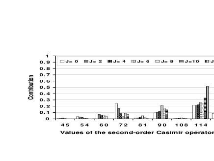
FIG. 1.: Strength distribution of $C_{2}$ of $SU(3)$ in yrast states of ${}^{44}Ti$ for realistic single particle energies with Kuo-Brown-3 two body interaction ($KB3$).

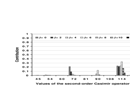
FIG. 2.: Strength distribution of $C_{2}$ of $SU(3)$ in yrast states of ${}^{44}Ti$ for degenerate single particle energies with Kuo-Brown-3 two body interaction ($KB3p\_f$).

We have chosen ${}^{44}Ti$ for an in-depth consideration of the fragmentation of the $C_{2}$ strength in yrast states. The results on the nondegenerate $KB3$ interaction are shown in Fig.1. In this case the highest contribution (biggest bar) is more than $50\%$ which corresponds to a $C_{2}$ value of 114 for the $J=12$ state. The $C_{2}=114$ value is for $(\lambda,\mu)=(8,2)$ which is two $SU(3)$ irreps down from the leading one, $(\lambda,\mu)=(12,0)$ with $C_{2}=180$. The leading irrep only contributes about 10$\%$ to the $J=12$ yrast state. The contribution of the next to the leading irrep, $C_{2}=144$ for $(\lambda,\mu)=(10,1)$, is slightly less than 40$\%$. Thus, for all practical purposes, the first three irreps determine the structure of the $J=12$ yrast state. This illustrates that the high total angular momentum $J$ states are composed of only the first few $SU(3)$ irreps. This is easily understood because high $J$ values require high orbital angular momentum $L$ which are only present in $SU(3)$ irreps with large $C_{2}$ values. The high $J$ states may therefore be considered to be states with good $SU(3)$ symmetry. However, this is not the case with the ground state of ${}^{44}Ti$ which has very important contributions from states with $C_{2}$ values 60, 72, 90, 114, 144, and 180 with respective percentages, 7.5, 25, 10, 21, 8, and 21$\%$. This shows that the leading irrep is not the biggest contributor to the $J=0$ ground state; there are two other contributors with about $20\%$, the third ($C_{2}=114$) and seventh ($C_{2}=72$) $SU(3)$ irrep.

When the spin-orbit interaction is turned off, which yields nearly degenerate single-particle energies since the single-particle orbit-orbit splitting is small, one has the $KB3p\_f$ interaction and in this case the structure of the yrast states changes dramatically, as shown in Fig.2. From Fig.2 one can see that the leading irrep plays a dominant role as its contribution is now more then $50\%$ of every yrast state. As in the previous case, the high total angular momentum $J$ states have the biggest contributions from the leading irrep, for example, more than 97$\%$ for $J=12$, 91$\%$ for $J=10$, and 80$\%$ for $J=8$. The ground state is composed of few irreps with $C_{2}$ values 72, 114, and 180, but in this case the leading irrep with $C_{2}=180$ makes up more than 52$\%$ of the total with the other two most important irreps contributing 21$\%$ [$C_{2}=72$, $(\lambda,\mu)=(4,4)]$ and 23$\%$ [$C_{2}=114$, $(\lambda,\mu)=(8,2)].$

An alternative way to show these results is given in Fig.3 and Fig.4. These figures show the centroid, width, and skewness of the $C_{2}$ distributions. The $J$ values are plotted on the horizontal axis with the centroids given on the vertical axis. The width of the distribution is indicated by the length of the error bars which is just the rms deviation, $\Delta C_{2}=\sqrt{\left\langle\left(C_{2}-\left\langle C_{2}\right\rangle\right)^{2}\right\rangle}$, from the average value of the second-order Casimir operator $\left\langle C_{2}\right\rangle$. The third central moment, $\delta C_{2}=\sqrt[3]{\left\langle\left(C_{2}-\left\langle C_{2}\right\rangle\right)^{3}\right\rangle}$, which measures the asymmetry, is indicated by the length of the error bar above, $\Delta C_{2}+\frac{\delta C_{2}}{2}$, and below, $\Delta C_{2}-\frac{\delta C_{2}}{2}$, the average value.

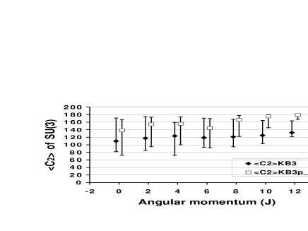
FIG. 3.: Average $C_{2}$ values for $KB3$ and $KB3p\_f$ interactions in ${}^{44}Ti$.

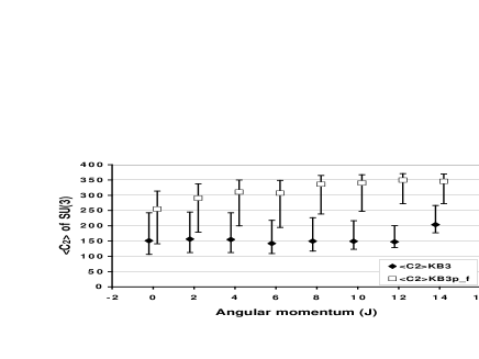
FIG. 4.: Average $C_{2}$ values for $KB3$ and $KB3p\_f$ interactions in ${}^{48}Ti$.

Note that the recovery of the leading irrep when the spin-orbit interaction is turned off is clearly signaled not only through an increase in the absolute values of the first centroid $\left\langle C_{2}\right\rangle$ but also through the skewness $\delta C_{2}$. For example, in ${}^{44}Ti$ with the $KB3$ interaction (spin-orbit interaction turned on) the ground state $J=0$ has $\left\langle C_{2}\right\rangle=110$ and skewness $\delta C_{2}=33$. This changes for the $KB3p\_f$ interaction to $\left\langle C_{2}\right\rangle=139$ and a skewness of $\delta C_{2}=-37$, as shown in Fig.3. The equivalent of the ${}^{44}Ti$ graph for the ${}^{48}Ti$ case is shown in Fig.4. As for the ${}^{44}Ti$ case, the results show the recovery of the $SU(3)$ symmetry in ${}^{48}Ti$ when the single-particle spin-orbit interaction is turned off.

We now turn to a discussion of the coherence nature of the yrast states. First notice that the widths of the distributions as defined by $\Delta C_{2}=\sqrt{\left\langle\left(C_{2}-\left\langle C_{2}\right\rangle\right)^{2}\right\rangle}$ are surprisingly unaffected (Fig.3 and Fig.4) by turning the spin-orbit interaction on and off. This effect occurs in all cases studied: ${}^{44}Ti,$ ${}^{46}Ti,$ ${}^{48}Ti$, and ${}^{48}Cr$. The more detailed graphs, Fig.1 and Fig.2, offer an explanation in terms of the fragmentation of the $C_{2}$ distribution. As can be seen from these graphs, the irreps that are presented in the structure of a given yrast state in the presence of the spin-orbit interaction (Fig.1) remain present, even though with reduced strength, in the structure of the state when the spin-orbit interaction is turned off (Fig.2). As a consequence, $\Delta C_{2}=\sqrt{\left\langle\left(C_{2}-\left\langle C_{2}\right\rangle\right)^{2}\right\rangle}$ which measures the overall spread of contributing irreps, is more or less independent of the spin-orbit interaction. One can see a sharp decrease in the width of the distribution only for high spin states like $J=12$ in the graph for ${}^{44}Ti$ in Fig.3.

The third type of graph, Fig.5, demonstrates the coherent nature of the states within the yrast band. The three graphs shown give the spectrum of the second-order Casimir operator $C_{2}$ of $SU(3)$ for the $J=0$, 2 and 4 yrast states in ${}^{48}Cr$. The axes are labelled the same way as in Figs.1 and 2, but in this case all bars are for a single yrast state. In this figure there are three peaks surrounded by smaller bars that yield a very similar enveloping shape for the given yrast states. The fragmentation and spread of $C_{2}$ values is nearly identical for these states with no dominant irrep, indicative of severe $SU(3)$ symmetry breaking.

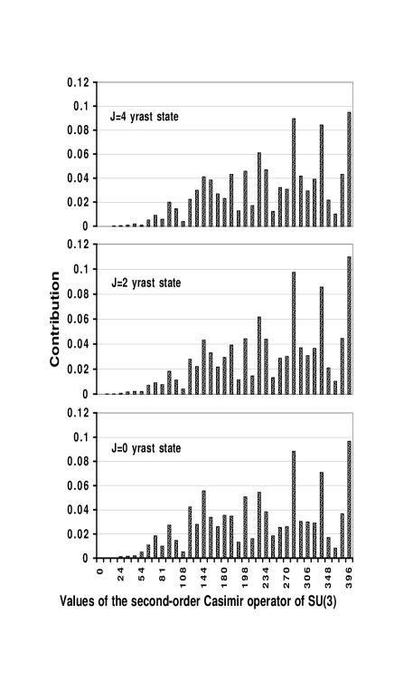
FIG. 5.: Coherent structure of the first three yrast states in ${}^{48}Cr$ calculated using realistic single particle energies with Kuo-Brown-3 two body interaction ($KB3$). On the horizontal axis is $C_{2}$ of $SU(3)$ with contribution of each $SU(3)$ state to the corresponding yrast state on the vertical axis.

Graphs for the $KB3p\_f$ case, when the spin-orbit interaction is turned off, are not shown since the results are similar to the results for ${}^{44}Ti$ shown in Fig.2. For example, when the spin-orbit interaction is on (KB3) the leading irrep for ${}^{48}Cr$ has a $C_{2}$ value of 396 and this account for only around 10$\%$ of the total strength distribution (see Fig.5), but when the spin-orbit interaction is off (KB3$p\_f$) the leading irrep is the dominant irrep with more than 55% of the total strength.

The last type of graph, Figs.6, 7, and 8 shows relative $B(E2)$ values, that is, $B(E2)$ strengths normalized to the $B(E2:2^{+}\rightarrow 0^{+})$ value. For isoscalar transitions the relative $B(E2)$ strengths are insensitive to the effective charges which may be used to bring the theoretical $B(E2:2^{+}\rightarrow 0^{+})$ numbers into agreement with the experimental values. Whenever an absolute $B(E2:2^{+}\rightarrow 0^{+})$ values are given they are in $e^{2}fm^{4}$ units and the effective charges are $1.5e$ for protons and $0.5e$ for neutrons ($q_{eff}$ = 0.5).

The first graph on relative $B(E2)$ values ( Fig.6 ) recaps our results for ${}^{44}Ti$. Calculated relative $B(E2)$ values for ${}^{44}Ti$ corresponding to the spin-orbit interaction turned on (KB3) and spin-orbit interaction off (KB3$p\_f$) are very close to the pure $SU(3)$ limit. The agreement with experiment is very satisfactory except for the $4^{+}\rightarrow 2^{+}$ and $8^{+}\rightarrow 6^{+}$ transitions. However, the experimental data [16] on $8^{+}\rightarrow 6^{+}$ transition gives only an upper limit of 0.5 pico-seconds to the half-life. We have used the worse case, namely a half-life of 0.5 ps, as a smaller value would increase the relative $B(E2)$ value. For example a half-life of 0.05 ps will agree well with the relative $B(E2)$ value for the $KB3p\_f$ interaction. This example supports the adiabatic mixing which seems to be present for all the yrast states of ${}^{44}Ti.$

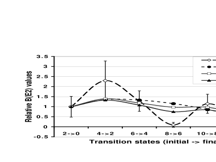
FIG. 6.: Relative $B(E2)$ values $\left(\frac{B(E2:J_{i}\rightarrow J_{f})}{B(E2:2^{+}\rightarrow 0^{+})}\right)$ for ${}^{44}Ti.$ The $B(E2:2^{+}\rightarrow 0^{+})$ transition values are 122.69$e^{2}fm^{4}$ from experiment, 104.82$e^{2}fm^{4}$ for the KB3 interaction, and 138.58$e^{2}fm^{4}$ for the $KB3p\_f$ case.

Fig.7 shows $B(E2)$ values for ${}^{46}Ti$. In this case there are deviations from adiabatic mixing for the $6^{+}\rightarrow 4^{+}$, $10^{+}\rightarrow 8^{+}$, and higher transitions. Two experimental data sets are shown in Fig.7: data from the NNDC is denoted as Exp_(NNDC), and updated data on $2^{+}\rightarrow 0^{+}$ and $4^{+}\rightarrow 2^{+}$ transitions from [18] is denoted as Exp_(Updated). For ${}^{46}Ti$ the agreement with the experiment is not as good as for ${}^{44}Ti$, however the experimental situation is also less certain. However, the coherent structure is well demonstrated for the first three yrast states $0^{+},$ $2^{+}$, and $4^{+}$ via relative $B(E2)$ values for the KB3 and $KB3p\_f$ interactions which are very close to the $SU\left(3\right)$ limit.

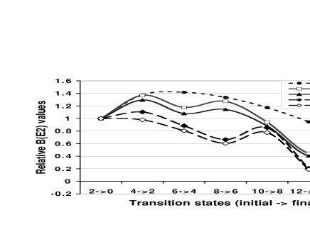
FIG. 7.: Relative $B(E2)$ values $\left(\frac{B(E2:J_{i}\rightarrow J_{f})}{B(E2:2^{+}\rightarrow 0^{+})}\right)$ for ${}^{46}Ti.$ The $B(E2:2^{+}\rightarrow 0^{+})$ transition values are 199.82$e^{2}fm^{4}$ from experimental data, 181.79$e^{2}fm^{4}$ from updated experimental data, 208$e^{2}fm^{4}$ for KB3 interaction, and 299.83$e^{2}fm^{4}$ for $KB3p\_f.$

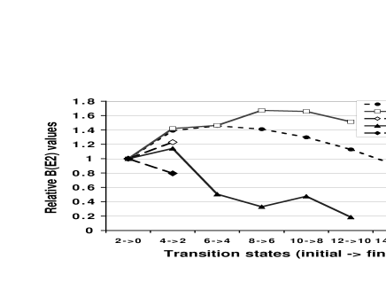
FIG. 8.: Relative $B(E2)$ values $\left(\frac{B(E2:J_{i}\rightarrow J_{f})}{B(E2:2^{+}\rightarrow 0^{+})}\right)$ for ${}^{48}Ti.$ The $B(E2:2^{+}\rightarrow 0^{+})$ transition values are 144.23$e^{2}fm^{4}$ from experimental data, 155.5$e^{2}fm^{4}$ from updated experimental data, 202.4$e^{2}fm^{4}$ for KB3 interaction, and 445.32$e^{2}fm^{4}$ for $KB3p\_f.$

We conclude this section by showing the recovery of the $SU(3)$ symmetry; this time via relative $B(E2)$ values as shown for ${}^{48}Ti$ in Fig.8. In Fig.8 we see that for the degenerate single particles case (KB3$p\_f$) the first few transitions have relative $B(E2)$ values which follow the $SU(3)$ limit very closely. On other hand, the interaction involving spin-orbit splitting (KB3) is far from the $SU(3)$ limit. The $B(E2:4^{+}\rightarrow 2^{+})$ transition is strongly enhanced due to the adiabatic mixing which is missing in the higher than $J=4$ yrast states.

V Conclusion and discussion

The results reported in this paper show that the single-particle spin-orbit splitting is the primary interaction responsible for breaking of the $SU(3)$ symmetry for nuclei in the lower $fp$-shell. When the spin-orbit splitting is reduced, as in the $KB3p\_f$ case, the importance of $SU(3)$ as seen through the dominance of the leading irrep represented in each yrast state is revealed. It is important to note in this regard that the $p$- and $f$-shells are nearly degenerate, which implies a small $l^{2}$ splitting.

Although the $SU(3)$ structure of the states is lost in the lower $fp$-shell, the results also show the mixing of $SU(3)$ irreps that occurs displays enhanced $B(E2)$ strengths. This adiabatic mixing results in a coherent structure that is represented in all yrast states for the ${}^{44}Ti$ case, while for the other nuclei studied this coherence breaks down after the first few yrast states. In particular, even though the yrast states are not dominated by a single $SU(3)$ irrep, the $B(E2:4^{+}\rightarrow 2^{+})$ values remain strongly enhanced with values close (usually within 10-20%) to the $SU(3)$ symmetry limit.

Support provided by the Department of Energy under Grant No. DE-FG02-96ER40985 and by the National Science Foundation under Grant No. PHY-9970769 and Cooperative Agreement EPS-9720652 that includes matching from the Louisiana Board of Regents Support Fund. The authors also wish to acknowledge the [Department of Energy’s] Institute for Nuclear Theory at the University of Washington for its hospitality during the final stage of completion of this work.

REFERENCES

-
[1]
J. M. Jauch and E. L. Hill, Phys. Rev. 57, 641
(1940);
H. J. Lipkin, “Lie Groups for Pedestrians,” North-Holland Publishing Company, Amsterdam (1966). -
[2]
J. P. Elliott, Proc. Roy. Soc. London Ser. A
245, 128 (1958); A 245, 562 (1958);
J. P. Elliott and H. Harvey, Proc. Roy. Soc. London Ser. A 272, 557 (1963);
J. P. Elliott and C. E. Wilsdon Proc. Roy. Soc. London Ser. A 302, 509 (1968). -
[3]
M. Goeppert Meyer, Phys. Rev. 75,
1969 (1949); 78, 16 (1950); 78, 22 (1950);
O. Haxel, J. H. D. Jensen, and H. E. Suess, Phys. Rev. 75, 1766 (1949). -
[4]
A. Bohr, B. R. Mottelson, and D.
Pines, Phys. Rev. 110, 936 (1958);
S. T. Belyaev, Mat. Fys. Medd. 31, 11 (1959). -
[5]
R. D. Ratnu Raju, J. P. Draayer, and K. T.
Hecht, Nucl. Phys. A202, 433 (1973);
A. Arima, M. Harvey and K. Shimizu, Phys. Lett. 30B, 517 (1969);
K.T. Hecht and A. Adler, Nucl. Phys. A137, 129 (1969);
R. F. Casten et al, “Algebraic Approaches to Nuclear Structure,” 1993 (Harwood, NY);
A. L. Blokhin, C. Bahri and J. P. Draayer, Phys. Rev. Let. 74, 4149 (1995). -
[6]
J. P. Draayer, K. J.
Weeks, and K. T. Hecht, Nucl. Phys. A381, 1 (1982);
O. Castaños, M. Moshinsky, and C. Quesne, Phys. Lett. B277, 238 (1992);
J. Dudek, W. Nazarewicz, Z. Szymanski and G. A. Leander, Phys. Rev. Lett. 59, 1405 (1987);
W. Nazarewicz, P. J. Twin, P. Fallon, and J. D. Garrett, Phys. Rev. Lett. 64, 1654 (1990). - [7] P. Ring and P. Schuck, “The Nuclear Many-Body Problem,” 1990 (Springer, NY).
-
[8]
P. Rochford and D.J. Rowe, Phys. Lett. B210, 5
(1988);
A. P. Zuker, J. Retamosa, A. Poves, and E. Caurier, Phys. Rev. C 52, R1741 (1995);
G. Mart nez-Pinedo, A. P. Zuker, A. Poves, and E. Caurier, Phys. Rev C 55, 187 (1997);
D.J. Rowe, C. Bahri, and W. Wijesundera, Phys. Rev. Lett. 80, 4394 (1998);
C. Bahri, D.J. Rowe, and W. Wijesundera, Phys. Rev. C 58, 1539 (1998);
A. Poves, J. Phys. G 25, 589 (1999);
C. Bahri and D.J. Rowe, Nucl. Phys. A662, 125 (2000);
D.J. Rowe, S. Bartlett, and C. Bahri, Physics Letters B 472, 227 (2000). -
[9]
T. Kuo and G. E. Brown, Nucl. Phys. A114, 241
(1968);
A. Poves and A. P. Zuker, Physics Reports 70, 235 (1981) - [10] J. Retamosa, J. M. Udias, A. Poves, and E. Moya de Guerra, Nucl. Phys. A511, 221 (1990).
- [11] B. A. Brown and B. H. Wildenthal, Ann. Rev. Nucl. Part. Sc. 36, 29 (1988).
- [12] R. R. Whitehead et al, Adv. Nucl. Phys. 9 123 (1977).
-
[13]
R. R. Whitehead and A. Watt, J. Phys. G 4, 835
(1978);
R. R. Whitehead et al, in “Theory and Application of Moment Methods in Many-Fermion Systems,” B. J. Dalton, et al, eds, Plenum Press, New York (1980);
E. Caurier, A. Poves, and A. P. Zuker, Phys. Lett B 252, 13 (1990);
E. Caurier, A. Poves, A. P. Zuker, Phys. Rev. Lett. 74, 1517 (1995). -
[14]
T. de Forest, Jr and J. D. Walecka, Adv. Phys. 15, 1 (1966);
J. D. Walecka, Muon Physics, vol. 2, edited by V. W. Hughes and C. S. Wu (Academic Press, New York, 1975) p. 113;
T. W. Donnelly and W. C. Haxton, At. Data Nucl. Data Tables 23, 103 (1979);
D. R. Bes and R. A. Sorensen, Adv. Nucl. Phys. 2, 129 (1969);
M. Dufour and A. P. Zuker, Phys. Rev. C 54, 1641 (1996);
S. Cohen, R. D. Lawson, M. H. Macfarlane, S. P. Pandya, and M. Soga, Phys. Rev. 160, 903 (1967). - [15] Jerry P. Draayer and Yorck Leschber,“ Branching Rules for Unitary Symmetries of the Nuclear Shell Model”, (Louisiana State University, 1987)
- [16] Evaluated experimental nuclear structure data ENSDF, ed. by National Nuclear Data Center, Brookhaven National Laboratory, Upton, NY 11973, USA (as of May 2000). Updated experimental data were obtained via http://www.nndc.bnl.gov/nndc/nudat/
- [17] E. Caurier and A. P. Zuker, A. Poves and G. Mart nez-Pinedo, Phys. Rev. C 50, 225 (1994).
- [18] R. Ernst et al, Phys. Rev. Lett. 84, 416 (2000).