PARTIAL DYNAMICAL SYMMETRIES IN NUCLEI

Partial dynamical symmetries (PDS) are shown to be relevant to the interpretation of the $K=0_{2}$ band and to the occurrence of F-spin multiplets of ground and scissors bands in deformed nuclei. Hamiltonians with bosonic and fermionic PDS are presented.

1 Introduction

When a dynamical symmetry occurs all properties of the system (e.g. energy eigenvalues) and wave functions are known analytically thus providing clarifying insights into complex dynamics. The majority of nuclei, however, do not satisfy the predictions of exact dynamical symmetries. Instead, one often finds that only a subset of states fulfill the symmetry while other states do not. In such circumstances, referred to as partial symmetries, the Hamiltonian supports a coexistence of “special” solvable states and other states which are mixed. Examples of partial symmetries in nuclear spectra are discussed below.

2 Partial SU(3) symmetry and the nature of the $K=0_{2}$ band

The nature of the lowest K=$0^{+}$ [K=$0_{2}$] excitation in deformed nuclei is still subject to controversy. Traditionally described as a $\beta$ vibration, its properties are empirically erratic in contrast to the regular behavior observed for ground and $\gamma$ bands. This suggests different symmetry character for these bands. With that in mind, the following IBM $\!{}^{{\bf?}}$ Hamiltonian with partial SU(3) symmetry has been proposed $\!{}^{{\bf?}}$

$$H\;=\;h_{0}P^{\dagger}_{0}P_{0}+h_{2}P^{\dagger}_{2}\cdot\tilde{P}_{2}~{},$$ (1)

where $P^{\dagger}_{L}$ $(L=0,2)$ are boson-pairs. Although $H$ is not an $SU(3)$ scalar, it has solvable ground and $\gamma$ bands with good $SU(3)$ symmetry, $(\lambda,\mu)=(2N,0),\,(2N-4,2)$ respectively. In contrast, the $K=0_{2}$ band involves a mixture of $SU(3)$ irreps $(2N-4,2)$, $(2N-8,4)$ and $(2N-6,0)$ or equivalently a mixture of single-phonon ($\beta$) and double-phonon ($\gamma^{2}_{K=0}$ and $\beta^{2}$) components. The respective probability amplitudes $(A_{\beta})^{2}$, $(A_{\gamma^{2}})^{2}$, $(A_{\beta^{2}})^{2}$ are shown in Fig. 1.

Figure 1: Properties of the $K=0_{2}$ band as a function of $h_{0}/h_{2}$, parameters of the SU(3) PDS Hamiltonian, Eq. (1), N=16 (solid lines). The dotted and dot-dashed lines are approximations based on 3-band mixing calculation. (a) Ratio of $K=0_{2}$ and $\gamma$ bandhead energies. (b) Probability amplitudes squared, $(A_{\beta})^{2}$, $(A_{\gamma^{2}})^{2}$, $(A_{\beta^{2}})^{2}$ for the $K=0_{2}$ wave function. Figure taken from [3].

In the current PDS scheme both the SU(3) breaking and the double-phonon admixture in the $K=0_{2}$ wave function are given by $(1-A_{\beta}^{2})$. The mixing is of order ($1/N)$ but depends critically on the ratio of the $K=0_{2}$ and $\gamma$ bandhead energies (also shown in Fig. 1). For most of the relevant range of $h_{0}/h_{2}$, corresponding to bandhead ratio in the range $0.8-1.65$, the double-phonon admixture is at most $\sim 15\%$ ($12.5\%$ in ¹⁶⁸Er). These findings support the conventional single-phonon interpretation for the $K=0_{2}$ band with small but significant double-$\gamma$-phonon admixture.

Table 1: Comparison of theoretical and experimental absolute B(E2) values [W.u.] for transitions from the $2^{+}_{K=0_{2}}$ level [4] and to the $0^{+}_{K=0_{2}}$ level [5] in ¹⁶⁸Er.

Exp.			Calc.
Transition	B(E2)	range	PDS	WCD	CQF
Lifetime measurement [4]
$2^{+}_{K=0_{2}}\rightarrow 0^{+}_{g}$	0.4	0.06–0.94	0.65	0.15	0.03
$2^{+}_{K=0_{2}}\rightarrow 2^{+}_{g}$	0.5	0.07–1.27	1.02	0.24	0.03
$2^{+}_{K=0_{2}}\rightarrow 4^{+}_{g}$	2.2	0.4–5.1	2.27	0.50	0.10
$2^{+}_{K=0_{2}}\rightarrow 2^{+}_{\gamma}$ a)	6.2 (3.1)	1–15 (0.5–7.5)	4.08	4.16	4.53
$2^{+}_{K=0_{2}}\rightarrow 3^{+}_{\gamma}$ a)	7.2 (3.6)	1–19 (0.5–9.5)	7.52	7.90	12.64
Coulomb excitation [5]
$2^{+}_{g}\rightarrow 0^{+}_{K=0_{2}}$	$0.08\pm 0.01$		0.79	0.18	0.03
$2^{+}_{\gamma}\rightarrow 0^{+}_{K=0_{2}}$	$0.55\pm 0.08$		3.06	3.20	5.29

Since the wave functions of the solvable states are known, it is possible to obtain analytic expressions for the E2 rates between them $\!{}^{{\bf?},{\bf?}}$. B(E2) ratios for $\gamma\rightarrow g$ transitions are parameter-free predictions of SU(3) PDS, and have been used $\!{}^{{\bf?}}$ to establish the validity of this scheme in ¹⁶⁸Er. Absolute B(E2) values for $K=0_{2}\rightarrow g$ transitions can be used $\!{}^{{\bf?}}$ to extract $(A_{\beta})^{2}$. In Table 1 we compare the predictions of the PDS and broken-SU(3) calculations: added $O(6)$ term (WCD) and consistent-Q formalism (CQF), with the B(E2) values deduced from a lifetime measurement $\!{}^{{\bf?}}$ and Coulomb excitation $\!{}^{{\bf?}}$ in ¹⁶⁸Er. It is seen that the PDS and WCD calculations agree well with the lifetime measurement, but the CQF calculation under-predicts the $K=0_{2}\rightarrow g$ data. On the other hand, all calculations show large deviations from the quoted B(E2) values measured in Coulomb excitation. It should be noted, however, that there are serious discrepancies between the above two measurements $\!{}^{{\bf?}}$. An independent measurement of the lifetime of the $0^{+}_{K=0_{2}}$ in ¹⁶⁸Er is highly desirable to clarify this issue.

3 F-spin as a partial symmetry

F-spin characterizes the proton-neutron ($\pi$-$\nu$) symmetry of IBM-2 states. There are empirical indications $\!{}^{{\bf?}}$ that low lying collective states have predominantly $F=F_{max}=(N_{\pi}+N_{\nu})/2$ with typical impurities of $2\%-4\%$. In spite of its appeal, however, F-spin cannot be an exact symmetry of the Hamiltonian. The assumption of F-spin scalar Hamiltonians is at variance with the microscopic interpretation of the IBM-2, which necessitates different effective interactions between like and unlike nucleons. Furthermore, if F-spin was a symmetry of the Hamiltonian, then all states would have good F-spin and would be arranged in F-spin multiplets. Experimentally the latter are observed in ground bands but not necessarily in excited $\beta$ and $\gamma$ bands. Thus F-spin can at best be an approximate quantum number which is good only for a selected set of states. These are precisely the signatures of a partial symmetry.

Table 2: The ratio $R=\sum B(M1)\uparrow/(C_{F,F_{0}})^{2}$ for members of F-spin multiplets. Here $C_{F,F_{0}}=~{}(F,F_{0};1,0|F-1,F_{0})$. The low value of the summed M1 strength to the scissors mode $\sum B(M1)\uparrow$ for ¹⁷²Yb has been attributed to experimental deficiencies.

Nucleus	$F$	$F_{0}$	$\sum B(M1)\uparrow$ $[\mu_{N}^{2}]$	$(C_{F,F_{0}})^{2}$	$R$
148Nd	4	1	0.78 (0.07)	5/12	1.87 (0.17)
148Sm		2	0.43 (0.12)	1/3	1.29 (0.36)
150Nd	9/2	1/2	1.61 (0.09)	4/9	3.62 (0.20)
150Sm		3/2	0.92 (0.06)	2/5	2.30 (0.15)
154Sm	11/2	1/2	2.18 (0.12)	5/11	4.80 (0.26)
154Gd		3/2	2.60 (0.50)	14/33	6.13 (1.18)
160Gd	7	0	2.97 (0.12)	7/15	6.36 (0.26)
160Dy		1	2.42 (0.18)	16/35	5.29 (0.39)
162Dy	15/2	1/2	2.49 (0.13)	7/15	5.34 (0.28)
166Er		$-1/2$	2.67 (0.19)	7/15	5.72 (0.41)
164Dy	8	0	3.18 (0.15)	8/17	6.76 (0.32)
168Er		$-1$	3.30 (0.12)	63/136	7.12 (0.26)
172Yb		$-2$	1.94 (0.22)	15/34	4.40 (0.50)
170Er	17/2	$-3/2$	2.63 (0.16)	70/153	5.75 (0.35)
174Yb		$-5/2$	2.70 (0.31)	66/153	6.26 (0.72)

A class of IBM-2 Hamiltonians with such property has been proposed $\!{}^{{\bf?}}$

$$H = \sum_{i}\sum_{L=0,2}A^{(L)}_{i}R^{\dagger}_{i,L}\cdot\tilde{R}_{i,L}+B\hat{{\cal M}}_{\pi\nu}$$ (2)

The $R^{\dagger}_{i,L}$ ($L=0,2$) are boson pairs with $F=1,\,i=F_{0}=0,\pm 1$ and $\hat{{\cal M}}_{\pi\nu}$ is the Majorana operator. The above Hamiltonian is non-F-scalar but has a subset of solvable states which form F-spin multiplets for the $K=0$ ground band with $F=F_{max}$, and for the $K=1$ scissors band with $F=F_{max}-1$, while other excited bands are mixed. For ground bands such structures have been empirically established. Since the $M1$ operator $(\hat{L}_{\pi}-\hat{L}_{\nu})$ is an F-spin vector, the prediction for F-spin multiplets of scissors states can be tested by examining the ratio of summed ground to scissors $B(M1)$ strength divided by the square of the appropriate Clebsch Gordan coefficient. In Table 2 we list all F-spin partners for which $\sum B(M1)\uparrow$ has been measured todate. It is seen that within the experimental errors, the above ratio is, as expected, fairly constant. The solvable ground and scissors bands have the same moment of inertia in agreement with the conclusions of a recent comprehensive analysis of the scissors mode in heavy even-even nuclei $\!{}^{{\bf?}}$.

4 Fermionic Partial Symmetry

Partial symmetries are not confined to bosonic systems. A fermionic Hamiltonian with SU(3) partial symmetry has been proposed $\!{}^{{\bf?}}$ in the framework of the symplectic shell model $\!{}^{{\bf?}}$,

$$H(\beta_{0},\beta_{2})=\beta_{0}\hat{A}_{0}\hat{B}_{0}+\beta_{2}\hat{A}_{2}\cdot\hat{B}_{2}~{},$$ (3)

with a structure similar to that of the bosonic Hamiltonian of Eq. (1). The $\hat{A}_{L}$ ($\hat{B}_{L}$), $L$ = 0 or 2, are symplectic generators which create (annihilate) $2\hbar\omega$ excitations in the system. The above Hamiltonian is not SU(3) invariant but has a subset of solvable pure-SU(3) states (e.g. the $0\hbar\omega$ $K=0_{1}$ and $2\hbar\omega$ $K=2_{1}$ bands in Fig. 2). The PDS Hamiltonian (3) can be rewritten in terms of the symplectic quadrupole-quadrupole interaction $Q_{2}\cdot Q_{2}$ plus terms diagonal in the Sp(6,R) $\supset$ SU(3) $\supset$ SO(3) chain and terms coupling different harmonic oscillator shells. The eigenstates of the two Hamiltonians are compared in Fig. 2 with parameters tuned to the ground band of ²⁰Ne. For both the ground and the resonance bands, PDS eigenstates are seen to approximately reproduce the structure of the exact $Q_{2}\cdot Q_{2}$ eigenstates within the $0\hbar\omega$ and $2\hbar\omega$ spaces, respectively. In particular, for each pure state of the PDS scheme we find a corresponding eigenstate of the quadrupole-quadrupole interaction, which is dominated by the same SU(3) irrep. Moreover, for reasonable interaction parameters, each rotational band is primarily located in one level of excitation, with the exception of the lowest $K=0_{2}$ resonance band, which is spread over many $N\hbar\omega$ excitations.

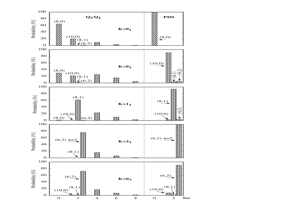
Figure 2: Decomposition for calculated $2^{+}$ states of ²⁰Ne. Individual contributions from the relevant SU(3) irreps at the 0$\hbar\omega$ and 2$\hbar\omega$ levels are shown for both a symplectic $8\hbar\omega$ calculation (denoted $Q_{2}\cdot Q_{2}$) and a PDS calculation. In addition, the total strengths contributed by the $N\hbar\omega$ excitations for $N>2$ are given for the symplectic case. Figure taken from [9].

References

References

- [1] F. Iachello and A. Arima, The Interacting Boson Model, (Cambridge Univ. Press, 1987).
- [2] A. Leviatan, Phys. Rev. Lett. 77, 818 ((1996).
- [3] A. Leviatan and I. Sinai, Phys. Rev. C 60, 061301 (1999).
- [4] H. Lehmann et al., Phys. Rev. C 57, 569 (1998).
- [5] T. Härtlein et al. Eur. Phys. J. A 2, 253 (1998).
- [6] P.O. Lipas, P. von Brentano and A. Gelberg, Rep. Prog. Phys. 53, 1355 (1990) and references therein.
- [7] A. Leviatan and J.N. Ginocchio, Phys. Rev. C 61, 24305 (2000).
- [8] J. Enders et al., Phys. Rev. C 59, R1851 (1999).
- [9] J. Escher and A. Leviatan, Phys. Rev. Lett. 84, 1866 (2000).
- [10] D. J. Rowe, Rep. Prog. Phys. 48, 1419 (1985).