Relativistic Quark Spin Coupling Effects in the Correlations Between Nucleon Electroweak Properties

Abstract

We investigate the effect of different relativistic spin couplings of constituent quarks on nucleon electroweak properties. Within each quark spin coupling scheme the correlations between static electroweak observables are found to be independent of the particular shape of the momentum part of the nucleon light-front wave function. The neutron charge form factor is very sensitive to different choices of spin coupling schemes once the magnetic moment is fitted to the experimental value. However, it is found rather insensitive to the details of the momentum part of the three-quark wave function model.

I Introduction

In a previous work[1], we have studied nucleon electromagnetic form factors using different forms of relativistic spin couplings between the constituent quarks forming the nucleon. We have used an effective Lagrangian to describe the quark spin coupling to the nucleon keeping close contact with covariant field theory. We have performed a three-dimensional reduction of the amplitude for the (virtual) photon absorption by the nucleon to the null-plane, $x^{+}=x^{0}+x^{3}=0$, (see, e.g., Ref. [2]). After the three-dimensional reduction the momentum part of the nucleon light-front wave function was introduced into the two-loop momentum integrations that define the matrix elements of the electromagnetic current.

In Ref. [1] we have tested different spin couplings for the nucleon in a calculation of nucleon electromagnetic form factors and found that the neutron charge form factor in particular leads to constraints of the quark spin coupling. The comparison with the neutron data below momentum transfer of 1 GeV/c suggests that the scalar pair is preferred in the relativistic quark spin coupling of the nucleon. That study was performed assuming the same Gaussian wave function for both the mixed scalar and gradient quark pair couplings.

Presently, while extending this investigation to other form factors we additionally introduce a power law behavior for the momentum part of the light-front wave function. The purpose is to investigate whether the neutron charge form factor is still reproduced with a scalar quark pair coupling while relaxing the form of the momentum part of the light-front wave function. This is indeed the case for both forms (Gaussian and power-law) once the magnetic moment of the neutron is fitted to its experimental value. Moreover, for a given quark spin coupling scheme and independent of the shape of the light-front wave function a model independent relation between the neutron charge radius and its magnetic moment can be recognized. We also present results on the nucleon axial vector form factor and on correlations between the static electroweak observables for different spin couplings and wave functions. In the context of the Bakamjian-Thomas (BT) quark spin coupling scheme it was shown that the axial vector coupling constant, the proton magnetic moment, and the radius are correlated by model independent relations[3, 4]. We point out that the high momentum transfer calculation of the nucleon electromagnetic form factors with that model were first done in Ref. [5]. We show that the different quark spin coupling schemes retain the model independent correlations found. However, the relations involving the axial vector coupling constant obtained with a spin coupling scheme from an effective Lagrangian differ from those derived within the Bakamjian-Thomas construction [3].

The effective Lagrangian for the N-q coupling is written as[1],

$${\cal{L}}_{\mathrm{N-3q}}=\alpha m_{N}\epsilon^{lmn}\overline{\Psi}_{(l)}i\tau_{2}\gamma^{5}\Psi_{(m)}^{C}\overline{\Psi}_{(n)}\Psi_{N}+(1-\alpha)\epsilon^{lmn}\overline{\Psi}_{(l)}i\tau_{2}\gamma_{\mu}\gamma^{5}\Psi_{(m)}^{C}\overline{\Psi}_{(n)}i\partial^{\mu}\Psi_{N}+H.C.$$ (1)

where $\tau_{2}$ is the isospin matrix, the color indices are $\{l,m,n\}$ and $\epsilon^{lmn}$ is the totally antisymmetric symbol. The conjugate quark field is $\Psi^{C}=C\overline{\Psi}^{\top}$, where $C=i\gamma^{2}\gamma^{0}$ is the charge conjugation matrix; $\alpha$ is a parameter to vary the relative magnitude of the spin couplings, and $m_{N}$ is the nucleon mass.

The macroscopic matrix elements of the nucleon electromagnetic current $J^{+}_{N}(q^{2})$ in the Breit-frame and in the light-front spinor basis is given by:

$$\langle s^{\prime}|J^{+}_{N}(q^{2})|s\rangle = \bar{u}(p^{\prime},s^{\prime})\left(F_{1N}(q^{2})\gamma^{+}+i\frac{\sigma^{+\mu}q_{\mu}}{2m_{N}}F_{2N}(q^{2})\right){u}(p,s)$$ (2)

$$= \frac{p^{+}}{m_{N}}\langle s^{\prime}|F_{1N}(q^{2})-i\frac{F_{2N}(q^{2})}{2m_{N}}\vec{q}_{\perp}\cdot(\vec{n}\times\vec{\sigma})|s\rangle\ ,$$ (3)

where $F_{1N}$ and $F_{2N}$ are the Dirac and Pauli form factors, respectively, while $\vec{n}$ is the unit vector along the $z$-direction. The Breit-frame momenta are $q=(0,\vec{q}_{\perp},0)$, such that $(q^{+}=q^{0}+q^{3}=0)$ and $\vec{q}_{\perp}=(q^{1},q^{2})$; $p=(\sqrt{q^{2}_{\perp}/4+m^{2}_{N}},-\vec{q}_{\perp}/2,0)$ and $p^{\prime}=(\sqrt{q^{2}_{\perp}/4+m^{2}_{N}},\vec{q}_{\perp}/2,0)$.

The Sachs form factors are defined by:

$$G_{EN}(q^{2}) = F_{1N}(q^{2})+\frac{q^{2}}{4m_{N}^{2}}F_{2N}(q^{2})\ ,$$ (4)

$$G_{MN}(q^{2}) = F_{1N}(q^{2})+F_{2N}(q^{2})\ .$$ (5)

The magnetic moment is $\mu_{N}=G_{MN}(0)$ and the mean squared radius is $r^{2}_{N}=6\frac{dG_{EN}(q^{2})}{dq^{2}}|_{q^{2}=0}$.

The non-vanishing part of the macroscopic matrix elements of the nucleon weak isovector axial vector current $A^{+}_{N}(q^{2})$ in the Breit-frame with $q^{+}=0$ in the light-front spinor basis is given by:

$$\langle s^{\prime}|A^{+}_{N}(q^{2})|s\rangle = \bar{u}(p^{\prime},s^{\prime})\left(G_{A}(q^{2})\gamma^{+}\gamma^{5}\frac{\vec{\tau}}{2}\right){u}(p,s)$$ (6)

$$= \frac{p^{+}}{m_{N}}G_{A}(q^{2})\langle s^{\prime}|\frac{\vec{\tau}}{2}\sigma_{z}|s\rangle\ ,$$ (7)

where $G_{A}$ is the weak isovector axial vector form factor and $g_{A}=G_{A}(0)$ is the axial vector coupling constant.

The light-front spinors are:

$$u(p,s)=\frac{\hbox to0.0pt{/\hss}p+m}{2\sqrt{p^{+}m}}\gamma^{+}\gamma^{0}\left(\begin{array}[]{c}\chi^{\rm Pauli}_{s}\\ 0\end{array}\right)\ .$$ (10)

The Dirac spinor of the instant form

$$u_{D}(p,s)=\frac{\hbox to0.0pt{/\hss}p+m}{\sqrt{2m(p^{0}+m)}}\left(\begin{array}[]{c}\chi^{\rm Pauli}_{s}\\ 0\end{array}\right)\$$ (13)

carries the subscript $D$. The Melosh rotation is the unitary transformation between the light-front and instant form spinors that is given by:

$$\left[R_{M}(p)\right]_{s^{\prime}s}\ =\langle s^{\prime}|\frac{p^{+}+m-i\vec{\sigma}.(\vec{n}\times\vec{p})}{\sqrt{(p^{+}+m)^{2}+p^{2}_{\perp}}}|s\rangle\ =\overline{u}_{D}(p,s^{\prime})u(p,s)\ ,$$ (14)

where $\vec{n}$ the unit vector along the z-direction.

In section II, the general form of the microscopic matrix elements of the nucleon electroweak current are discussed. The detailed form of the electromagnetic current is derived and the light-front wave function is introduced in the computation of the form factors. Also, the matrix element of the weak isovector axial vector current of the nucleon are derived from the effective Lagrangian. In section III, the physics of the different spin coupling schemes are discussed in comparison with the widely used Bakamjian-Thomas framework. In section IV, the numerical results of the static electroweak observables and of the form factors are presented. The model independence within each spin coupling scheme is demonstrated for the correlation between the static nucleon electroweak observables. In section V, we give the summary and conclusion.

II Nucleon electroweak current

The microscopic matrix elements of the nucleon electromagnetic and weak isovector axial vector currents are constructed from the effective Lagrangian given in Eq.(1). The current matrix elements are evaluated in impulse approximation. The complete antisymmetrization of the quark states implies four topologically distinct diagrams depicted in Figure 1. The two-loop triangle diagrams of Figure 1 represent the impulse approximation for the evaluation of the baryon form factors in light-front dynamics. We calculate the matrix elements of the currents via coupling to the third quark due to the symmetrization of the microscopic matrix element after factorizing the color degree of freedom. The electromagnetic quark current operator is $\overline{\Psi}\hat{Q}_{q}\gamma^{\mu}\Psi$, with $\hat{Q}_{q}$ the charge operator, and the weak isovector axial vector current one is $\overline{\Psi}\frac{\vec{\tau}}{2}\gamma^{\mu}\gamma^{5}\Psi$.

In detail, Figure 1a represents the nucleon spin-space operators $J^{+}_{aN}$ and $A^{+}_{aN}$. In these cases the elementary operators act on quark 3 while 1 and 2 compose the coupled spectator quark pair of Eq. (1) for the initial and final nucleons alike. In Figure 1b, the coupled quark pair of the initial nucleon is (13) whereas it is (12) in the final nucleon. The operators $J^{+}_{bN}$ and $A^{+}_{bN}$ represented by Figure 1b are multiplied by a factor of 4. A factor 2 comes from the exchange of quarks 1 and 2 and another factor 2 comes from the invariance under exchanging the pairs in the initial and final nucleons that is a consequence of time reversal and parity transformation properties. The operators $J^{+}_{cN}$ and $A^{+}_{cN}$ are represented by Figure 1c, where the initial coupled pair quark is (13) and the final coupled pair is (23). This operator is multiplied by a factor of 2 because quarks 1 and 2 can be exchanged. Finally, the process shown in Figure 1d does not contribute to the nucleon axial vector current because of the isoscalar quark pair as given by the Lagrangian of Eq.(1). However this diagram is non vanishing for the electromagnetic current and denoted by $J^{+}_{dN}$. It corresponds to the process in which the photon is absorbed by the coupled quark pair (13) while 2 is the spectator. In this case, two diagrams are possible by the exchange of quarks 1 and 2 giving rise to a factor of 2.

The microscopic operator of the nucleon electromagnetic current is given by the sum of four terms:

$$J^{+}_{N}(q^{2})=J^{+}_{aN}(q^{2})+4J^{+}_{bN}(q^{2})+2J^{+}_{cN}(q^{2})+2J^{+}_{dN}(q^{2}).$$ (15)

The weak isovector axial vector current has contribution from three terms:

$$A^{+}_{N}(q^{2})=A^{+}_{aN}(q^{2})+4A^{+}_{bN}(q^{2})+2A^{+}_{cN}(q^{2})\ .$$ (16)

The term $A^{+}_{dN}(q^{2})$ vanishes because of isospin properties.

A Derivation of the Electromagnetic Current Matrix Elements

The nucleon current operators $J^{+}_{\beta N}$, $\beta=a,b,c,d$ and $A^{+}_{\gamma N}$, $\gamma=a,b,c$ of Eqs. (15) and (16) are constructed directly from the Feynman diagrams of Figure 1. The electromagnetic current $J^{+}_{N}$ receives contributions from each amplitude represented by the Feynman two-loop triangle diagrams of Figures 1a to 1d, which we repeat here[1]:

$$\langle s^{\prime}|J^{+}_{aN}(q^{2})|s\rangle = -\langle N|\hat{Q}_{q}|N\rangle{\mathrm{Tr}}[i\tau_{2}(-i)\tau_{2}]\int\frac{d^{4}k_{1}d^{4}k_{2}}{(2\pi)^{8}}\Lambda(k_{i},p^{\prime})\Lambda(k_{i},p)\bar{u}(p^{\prime},s^{\prime})S(k^{\prime}_{3})\gamma^{+}$$ (17)

$$\times S(k_{3})u(p,s){\mathrm{Tr}}\left[S(k_{2})\left(\alpha m_{N}+(1-\alpha)\hbox to0.0pt{/\hss}p\right)\gamma^{5}S_{c}(k_{1})\gamma^{5}\left(\alpha m_{N}+(1-\alpha)\hbox to0.0pt{/\hss}p^{\prime}\right)\right]\ ,$$ (18)

with $\displaystyle S(p)=\frac{1}{\hbox to0.0pt{/\hss}p-m+i\epsilon}\,,$ and $\displaystyle S_{c}(p)=\left[\gamma^{0}\gamma^{2}\frac{1}{\hbox to0.0pt{/\hss}p-m+i\epsilon}\gamma^{0}\gamma^{2}\right]^{\top}\,$. Here $m$ is the constituent quark mass and $k^{\prime}_{3}=k_{3}+Q\,$, and $\langle N|\hat{Q}_{q}|N\rangle$ is the isospin matrix. The function $\displaystyle\Lambda(k_{i},p)$ is chosen to introduce the momentum part of the three-quark light-front wave function, after the integrations over $k^{-}$ are performed. The contribution to the electromagnetic current represented by Figure 1b is given by:

$$\langle s^{\prime}|J^{+}_{bN}(q^{2})|s\rangle = -\langle N|\hat{Q}_{q}|N\rangle\int\frac{d^{4}k_{1}d^{4}k_{2}}{(2\pi)^{8}}\Lambda(k_{i},p^{\prime})\Lambda(k_{i},p)\bar{u}(p^{\prime},s^{\prime})S(k^{\prime}_{3})\gamma^{+}S(k_{3})$$ (19)

$$\times \left(\alpha m_{N}+(1-\alpha)\hbox to0.0pt{/\hss}p\right)\gamma^{5}S_{c}(k_{1})\gamma^{5}\left(\alpha m_{N}+(1-\alpha)\hbox to0.0pt{/\hss}p^{\prime}\right)S(k_{2})u(p,s)\ .$$ (20)

The contribution to the electromagnetic current represented by Figure 1c is given by:

$$\langle s^{\prime}|J^{+}_{cN}(q^{2})|s\rangle = \langle N|\tau_{2}\hat{Q}_{q}\tau_{2}|N\rangle\int\frac{d^{4}k_{1}d^{4}k_{2}}{(2\pi)^{8}}\Lambda(k_{i},p^{\prime})\Lambda(k_{i},p)\bar{u}(p^{\prime},s^{\prime})S(k_{1})\left(\alpha m_{N}+(1-\alpha)\hbox to0.0pt{/\hss}p\right)$$ (21)

$$\times \gamma^{5}S_{c}(k_{3})\gamma^{+}S_{c}(k^{\prime}_{3})\gamma^{5}\left(\alpha m_{N}+(1-\alpha)\hbox to0.0pt{/\hss}p^{\prime}\right)S(k_{2})u(p,s)\ .$$ (22)

The contribution to the electromagnetic current represented by Figure 1d is given by:

$$\langle s^{\prime}|J^{+}_{dN}(q^{2})|s\rangle = -{\mathrm{Tr}}[\hat{Q}_{q}]\int\frac{d^{4}k_{1}d^{4}k_{2}}{(2\pi)^{8}}\Lambda(k_{i},p^{\prime})\Lambda(k_{i},p)\bar{u}(p^{\prime},s^{\prime})S(k_{2})u(p,s)$$ (24)

$${\mathrm{Tr}}\left[\gamma^{5}\left(\alpha m_{N}+(1-\alpha)\hbox to0.0pt{/\hss}p^{\prime}\right)S(k^{\prime}_{3})\gamma^{+}S(k_{3})\left(\alpha m_{N}+(1-\alpha)\hbox to0.0pt{/\hss}p\right)\gamma^{5}S_{c}(k_{1})\right]\ .$$

The light-front coordinates are defined as $k^{+}=k^{0}+k^{3}\ ,k^{-}=k^{0}-k^{3}\ ,k_{\perp}=(k^{1},k^{2}).$ In each term of the nucleon current, from $J^{+}_{aN}$ to $J^{+}_{dN}$, the Cauchy integrations over $k^{-}_{1}$ and $k^{-}_{2}$ are performed. That means the on-mass-shell pole of the Feynman propagators for the spectator particles 1 and 2 of the photon absorption process are taken into account. In the Breit-frame with $q^{+}=0$ there is a maximal suppression of light-front Z-diagrams in $J^{+}$ [6, 7]. Thus the components of the momentum $k^{+}_{1}$ and $k^{+}_{2}$ are bounded such that $0<k^{+}_{1}<p^{+}$ and $0<k^{+}_{2}<p^{+}-k^{+}_{1}$[8]. The four-dimensional integrations of Eqs.(18) to (24) are reduced to the three-dimensional ones of the null-plane.

After the integrations over the light-front energies the momentum part of the wave function is introduced into the microscopic matrix elements of the current by the substitution [1, 6]:

$$\frac{1}{2(2\pi)^{3}}\frac{\Lambda(k_{i},p)}{m^{2}_{N}-M^{2}_{0}}\rightarrow\Psi(M^{2}_{0})\ .$$ (25)

To study the model dependence we choose the harmonic wave function and a power-law form [3, 4],

$$\Psi_{\mathrm{HO}}=N_{\mathrm{HO}}\exp(-M^{2}_{0}/2\beta^{2}),\qquad\Psi_{\mathrm{Power}}=N_{\mathrm{Power}}(1+M^{2}_{0}/\beta^{2})^{-p}\ ,$$ (26)

and $\beta$ is the width parameter. The free three-quark mass $M_{0}$ is given below in Eq.(30). From perturbative QCD arguments a power-law fall-off with $p=3.5$ is predicted [4]. The relations between static electroweak observables are not sensitive to $p$ as long as $p>2$ [3]. We choose for our calculations $p=3$. Further, the same momentum wave function is chosen all N-q couplings, for simplicity. Note, that the mixed ($\alpha=1/2$) case could have different momentum dependencies for each spin coupling, however, we choose the same momentum functions just to keep contact with the BT approach.

The analytical integration of Eq.(18) of the $k^{-}$ components of the momenta yields:

$$\langle s^{\prime}|J^{+}_{aN}(q^{2})|s\rangle = 2p^{+2}\langle N|\hat{Q}_{q}|N\rangle\int\frac{d^{2}k_{1\perp}dk^{+}_{1}d^{2}k_{2\perp}dk^{+}_{2}}{k^{+}_{1}k^{+}_{2}k^{+\ 2}_{3}}\theta(p^{+}-k^{+}_{1})\theta(p^{+}-k^{+}_{1}-k^{+}_{2})$$ (29)

$${\mathrm{Tr}}\left[(\hbox to0.0pt{/\hss}k_{2}+m)\left(\alpha m_{N}+(1-\alpha)\hbox to0.0pt{/\hss}p\right)(\hbox to0.0pt{/\hss}k_{1}+m)\left(\alpha m_{N}+(1-\alpha)\hbox to0.0pt{/\hss}p^{\prime}\right)\right]$$

$$\bar{u}(p^{\prime},s^{\prime})(\hbox to0.0pt{/\hss}k^{\prime}_{3}+m))\gamma^{+}(\hbox to0.0pt{/\hss}k_{3}+m)u(p,s)\Psi(M^{{}^{\prime}2}_{0})\Psi(M^{2}_{0})\ ,$$

where $k^{2}_{1}=m^{2}$ and $k^{2}_{2}=m^{2}$. The free three-quark squared mass is defined by:

$$M^{2}_{0}=p^{+}(\frac{k_{1\perp}^{2}+m^{2}}{k^{+}_{1}}+\frac{k_{2\perp}^{2}+m^{2}}{k^{+}_{2}}+\frac{k_{3\perp}^{2}+m^{2}}{k^{+}_{3}})-{p^{2}_{\perp}}\ ,$$ (30)

and $M^{\prime 2}_{0}=M^{2}_{0}(k_{3}\rightarrow k^{\prime}_{3}\ ,\vec{p}_{\perp}\rightarrow\vec{p}^{\prime}_{\perp})$.

The other terms of the nucleon current, as given by Eqs. (20)-(24) are also integrated over the $k^{-}$ momentum components of particles 1 and 2 following the same steps used to obtain Eq.(29) from Eq.(18):

$$\langle s^{\prime}|J^{+}_{bN}(q^{2})|s\rangle = p^{+2}\langle N|\hat{Q}_{q}|N\rangle\int\frac{d^{2}k_{1\perp}dk^{+}_{1}d^{2}k_{2\perp}dk^{+}_{2}}{k^{+}_{1}k^{+}_{2}k^{+\ 2}_{3}}\theta(p^{+}-k^{+}_{1})\theta(p^{+}-k^{+}_{1}-k^{+}_{2})$$ (33)

$$\bar{u}(p^{\prime},s^{\prime})(\hbox to0.0pt{/\hss}k^{\prime}_{3}+m)\gamma^{+}(\hbox to0.0pt{/\hss}k_{3}+m)\left(\alpha m_{N}+(1-\alpha)\hbox to0.0pt{/\hss}p\right)(\hbox to0.0pt{/\hss}k_{1}+m)$$

$$\times\left(\alpha m_{N}+(1-\alpha)\hbox to0.0pt{/\hss}p^{\prime}\right)(\hbox to0.0pt{/\hss}k_{2}+m)u(p,s)\Psi(M^{{}^{\prime}2}_{0})\Psi(M^{2}_{0})\ ,$$

$$\langle s^{\prime}|J^{+}_{cN}(q^{2})|s\rangle = p^{+2}\langle N|\tau_{2}\hat{Q}_{q}\tau_{2}|N\rangle\int\frac{d^{2}k_{1\perp}dk^{+}_{1}d^{2}k_{2\perp}dk^{+}_{2}}{k^{+}_{1}k^{+}_{2}k^{+\ 2}_{3}}\theta(p^{+}-k^{+}_{1})\theta(p^{+}-k^{+}_{1}-k^{+}_{2})$$ (36)

$$\bar{u}(p^{\prime},s^{\prime})(\hbox to0.0pt{/\hss}k_{1}+m)\left(\alpha m_{N}+(1-\alpha)\hbox to0.0pt{/\hss}p\right)(\hbox to0.0pt{/\hss}k_{3}+m)\gamma^{+}(\hbox to0.0pt{/\hss}k^{\prime}_{3}+m)$$

$$\times\left(\alpha m_{N}+(1-\alpha)\hbox to0.0pt{/\hss}p^{\prime}\right)(\hbox to0.0pt{/\hss}k_{2}+m)u(p,s)\Psi(M^{{}^{\prime}2}_{0})\Psi(M^{2}_{0})\ ,$$

$$\langle s^{\prime}|J^{+}_{dN}(q^{2})|s\rangle = p^{+2}{\mathrm{Tr}}[\hat{Q}_{q}]\int\frac{d^{2}k_{1\perp}dk^{+}_{1}d^{2}k_{2\perp}dk^{+}_{2}}{k^{+}_{1}k^{+}_{2}k^{+\ 2}_{3}}\theta(p^{+}-k^{+}_{1})\theta(p^{+}-k^{+}_{1}-k^{+}_{2})$$ (39)

$${\mathrm{Tr}}\left[\left(\alpha m_{N}+(1-\alpha)\hbox to0.0pt{/\hss}p^{\prime}\right)(\hbox to0.0pt{/\hss}k^{\prime}_{3}+m)\gamma^{+}(\hbox to0.0pt{/\hss}k_{3}+m)\left(\alpha m_{N}+(1-\alpha)\hbox to0.0pt{/\hss}p\right)(\hbox to0.0pt{/\hss}k_{1}+m)\right]$$

$$\bar{u}(p^{\prime},s^{\prime})(\hbox to0.0pt{/\hss}k_{2}+m)u(p,s)\Psi(M^{{}^{\prime}2}_{0})\Psi(M^{2}_{0})\ .$$

The normalization is chosen such that the proton charge is unity.

B Derivation of the Axial Vector Current Matrix Elements

The weak isovector axial vector current $A^{+}_{N}$ receives contributions from each amplitude represented by the Feynman two-loop triangle diagrams of Figures 1a to 1c:

$$\langle s^{\prime}|A^{+}_{aN}(q^{2})|s\rangle = -\langle N|\frac{\vec{\tau}}{2}|N\rangle{\mathrm{Tr}}[i\tau_{2}(-i)\tau_{2}]\int\frac{d^{4}k_{1}d^{4}k_{2}}{(2\pi)^{8}}\Lambda(k_{i},p^{\prime})\Lambda(k_{i},p)\bar{u}(p^{\prime},s^{\prime})S(k^{\prime}_{3})\gamma^{+}\gamma^{5}$$ (40)

$$\times S(k_{3})u(p,s){\mathrm{Tr}}\left[S(k_{2})\left(\alpha m_{N}+(1-\alpha)\hbox to0.0pt{/\hss}p\right)\gamma^{5}S_{c}(k_{1})\gamma^{5}\left(\alpha m_{N}+(1-\alpha)\hbox to0.0pt{/\hss}p^{\prime}\right)\right]\ .$$ (41)

The contribution to the axial vector current represented by Figure 1b is given by:

$$\langle s^{\prime}|A^{+}_{bN}(q^{2})|s\rangle = -\langle N|\frac{\vec{\tau}}{2}|N\rangle\int\frac{d^{4}k_{1}d^{4}k_{2}}{(2\pi)^{8}}\Lambda(k_{i},p^{\prime})\Lambda(k_{i},p)\bar{u}(p^{\prime},s^{\prime})S(k^{\prime}_{3})\gamma^{+}\gamma^{5}S(k_{3})$$ (42)

$$\times \left(\alpha m_{N}+(1-\alpha)\hbox to0.0pt{/\hss}p\right)\gamma^{5}S_{c}(k_{1})\gamma^{5}\left(\alpha m_{N}+(1-\alpha)\hbox to0.0pt{/\hss}p^{\prime}\right)S(k_{2})u(p,s)\ .$$ (43)

The contribution to the axial vector current represented by Figure 1c is given by:

$$\langle s^{\prime}|A^{+}_{cN}(q^{2})|s\rangle = \langle N|\tau_{2}\frac{\vec{\tau}}{2}\tau_{2}|N\rangle\int\frac{d^{4}k_{1}d^{4}k_{2}}{(2\pi)^{8}}\Lambda(k_{i},p^{\prime})\Lambda(k_{i},p)\bar{u}(p^{\prime},s^{\prime})S(k_{1})\left(\alpha m_{N}+(1-\alpha)\hbox to0.0pt{/\hss}p\right)$$ (44)

$$\times \gamma^{5}S_{c}(k_{3})\gamma^{+}\gamma^{5}S_{c}(k^{\prime}_{3})\gamma^{5}\left(\alpha m_{N}+(1-\alpha)\hbox to0.0pt{/\hss}p^{\prime}\right)S(k_{2})u(p,s)\ .$$ (45)

The contribution to the axial vector current represented by Figure 1d vanishes because of the isoscalar nature of the coupled quark pair.

In each term of the nucleon axial vector current, from $A^{+}_{aN}$ to $A^{+}_{cN}$, the Cauchy integrations over $k^{-}_{1}$ and $k^{-}_{2}$ are performed as discussed in the previous section for the electromagnetic current. The spectator particles are on their mass-shell after the integrations on the $k^{-}$ momentum in Eqs. (41) to (45). The numerators of the Dirac propagators of quark 3 on which the axial operator $\gamma^{+}\gamma^{5}$ acts have the momenta $k^{\prime}_{3}$ and $k_{3}$ on the $k^{-}$-shell because $(\gamma^{+})^{2}=0$. The components of the momentum $k^{+}_{1}$ and $k^{+}_{2}$ are bounded by $0<k^{+}_{1}<p^{+}$ and $0<k^{+}_{2}<p^{+}-k^{+}_{1}$[8]. The four-dimensional integrations of Eqs.(41) to (45) are reduced to the three dimensions of the null-plane.

The analytical integration of Eq.(41) of the $k^{-}$ components of the momenta yields:

$$\langle s^{\prime}|A^{+}_{aN}(q^{2})|s\rangle = 2p^{+2}\langle N|\frac{\vec{\tau}}{2}|N\rangle\int\frac{d^{2}k_{1\perp}dk^{+}_{1}d^{2}k_{2\perp}dk^{+}_{2}}{k^{+}_{1}k^{+}_{2}k^{+\ 2}_{3}}\theta(p^{+}-k^{+}_{1})\theta(p^{+}-k^{+}_{1}-k^{+}_{2})$$ (48)

$${\mathrm{Tr}}\left[(\hbox to0.0pt{/\hss}k_{2}+m)\left(\alpha m_{N}+(1-\alpha)\hbox to0.0pt{/\hss}p\right)(\hbox to0.0pt{/\hss}k_{1}+m)\left(\alpha m_{N}+(1-\alpha)\hbox to0.0pt{/\hss}p^{\prime}\right)\right]$$

$$\bar{u}(p^{\prime},s^{\prime})(\hbox to0.0pt{/\hss}k^{\prime}_{3}+m))\gamma^{+}\gamma^{5}(\hbox to0.0pt{/\hss}k_{3}+m)u(p,s)\Psi(M^{{}^{\prime}2}_{0})\Psi(M^{2}_{0})\ ,$$

and $k^{2}_{1}=m^{2}$ and $k^{2}_{2}=m^{2}$.

The integrations in the light-front energies in Eqs. (43) and (45) lead to:

$$\langle s^{\prime}|A^{+}_{bN}(q^{2})|s\rangle = p^{+2}\langle N|\frac{\vec{\tau}}{2}|N\rangle\int\frac{d^{2}k_{1\perp}dk^{+}_{1}d^{2}k_{2\perp}dk^{+}_{2}}{k^{+}_{1}k^{+}_{2}k^{+\ 2}_{3}}\theta(p^{+}-k^{+}_{1})\theta(p^{+}-k^{+}_{1}-k^{+}_{2})$$ (51)

$$\bar{u}(p^{\prime},s^{\prime})(\hbox to0.0pt{/\hss}k^{\prime}_{3}+m)\gamma^{+}\gamma^{5}(\hbox to0.0pt{/\hss}k_{3}+m)\left(\alpha m_{N}+(1-\alpha)\hbox to0.0pt{/\hss}p\right)(\hbox to0.0pt{/\hss}k_{1}+m)$$

$$\times\left(\alpha m_{N}+(1-\alpha)\hbox to0.0pt{/\hss}p^{\prime}\right)(\hbox to0.0pt{/\hss}k_{2}+m)u(p,s)\Psi(M^{{}^{\prime}2}_{0})\Psi(M^{2}_{0})\ ,$$

$$\langle s^{\prime}|A^{+}_{cN}(q^{2})|s\rangle = p^{+2}\langle N|\tau_{2}\frac{\vec{\tau}}{2}\tau_{2}|N\rangle\int\frac{d^{2}k_{1\perp}dk^{+}_{1}d^{2}k_{2\perp}dk^{+}_{2}}{k^{+}_{1}k^{+}_{2}k^{+\ 2}_{3}}\theta(p^{+}-k^{+}_{1})\theta(p^{+}-k^{+}_{1}-k^{+}_{2})$$ (54)

$$\bar{u}(p^{\prime},s^{\prime})(\hbox to0.0pt{/\hss}k_{1}+m)\left(\alpha m_{N}+(1-\alpha)\hbox to0.0pt{/\hss}p\right)(\hbox to0.0pt{/\hss}k_{3}+m)\gamma^{+}\gamma^{5}(\hbox to0.0pt{/\hss}k^{\prime}_{3}+m)$$

$$\times\left(\alpha m_{N}+(1-\alpha)\hbox to0.0pt{/\hss}p^{\prime}\right)(\hbox to0.0pt{/\hss}k_{2}+m)u(p,s)\Psi(M^{{}^{\prime}2}_{0})\Psi(M^{2}_{0})\ ,$$

III Discussion of Spin Coupling Schemes

The physical meaning of the effective Lagrangian for the quark spin coupling emerges if one performs a kinematical light-front boost of the matrix elements of the spin operators between quark states on one hand and quark-nucleon states related to the initial and final nucleons with their respective rest frames on the other hand. This has been suggested in Ref.[9] and also discussed in Ref.[1]. The effective Lagrangian of Eq.(1) contains the spin-flavor invariants of the nucleon with quark pair spin zero ($\alpha=1$) and spin one ($\alpha=0$) that are 2 of a basis of 8 such states given in detail in Ref. [10]. The nucleon spin invariant that is widely used and tested in form factor calculations uses the ones chosen here but contain the additional projector $\hbox to0.0pt{/\hss}p+M_{0}$ onto large Dirac components, a characteristic feature of the Bakamjian-Thomas (BT) spin coupling scheme [11]. The spin-flavor invariant of the effective Lagrangian Eq. (1) with $\alpha=1/2$ resembles the BT spin coupling scheme but is not equivalent to it, i.e., the Melosh rotations have their arguments defined in the nucleon rest frame with individual ’+’ momentum constrained by the total nucleon $p^{+}$. The BT construction have the Melosh spin rotation with the individual ’+’ momentum constrained by the free three-quark mass $M_{0}$. That differs from the above Lagrangian as explicitly shown in Ref.[9]. Moreover, in the pointlike nucleon limit, the weak isovector axial vector coupling constant represents a situation in which the difference between BT and effective Lagrangian spin coupling schemes is maximized as we will discuss at the end of this section.

The Melosh rotations appear in the equations for the vector and axial vector current from the residues of the triangle Feynman diagram, which are evaluated at the on-$k^{-}$-shell poles of the spectator particles, and each of the numerators of the Dirac propagator are on-$k^{-}$-shell. In particular, the numerator of quark 3 comes to be on-$k^{-}$-shell because $(\gamma^{+})^{2}=0$. Consequently, the numerators of the fermion propagators are substituted by the positive energy spinor projector, written in terms of light-front spinors. We use that the Wigner rotation is unity for kinematical Lorentz transformations to calculate the spin matrix elements of the nucleon current corresponding to the respective rest-frames of the initial or final nucleon. A typical matrix element of the spin coupling coefficient for $\alpha=1$ appearing in the evaluation of $J^{+}$ as well as in $A^{+}$, when calculated in the nucleon rest frame, is given by:

$$\chi(s_{1},s_{2},s_{3};s_{N})=\overline{u}_{1}\gamma^{5}u_{2}^{C}\;\overline{u}_{3}u_{N}\ ,$$ (55)

where $u_{i}=u(k_{i},s_{i})$ is the light-front spinor for the $i$-th quark.

The matrix element of the pair coupled to spin zero in Eq. (55) is evaluated in the rest frame of the pair (c.m.) reached by a kinematical light-front boost from the nucleon rest frame. The Wigner rotation is unity for such a Lorentz transformation consequently (viz. ${u}_{\rm c.m.}(\vec{k}^{{\rm c.m.}},s)={u}(\vec{k}^{{\rm c.m.}},s)$):

$$I(s_{1},s_{2},0) = \overline{u}(\vec{k}_{1},s_{1})\gamma^{5}u^{C}(\vec{k}_{2},s_{2})$$ (56)

$$= \overline{u}(\vec{k}^{{\rm c.m.}}_{1},s_{1})\gamma^{5}u^{C}(\vec{k}^{{\rm c.m.}}_{2},s_{2})\ ,$$ (57)

where the particle momenta in the pair (12) rest frame are $\vec{k}^{{\rm c.m.}}=(k^{+{\rm c.m.}},{\vec{k}}_{\perp}^{{\rm c.m.}})$ obtained from $k^{{\rm(c.m.)}\mu}=(\Lambda k)^{\mu}$. The operator $\Lambda$ is the kinematical light-front transformation from the nucleon rest frame to the pair rest frame. Introducing the completeness relation for positive energy Dirac spinors in Eq. (57), one finds:

$$I(s_{1},s_{2},0) = \sum_{\bar{s}_{1}\bar{s}_{2}}\overline{u}(\vec{k}^{{\rm c.m.}}_{1},s_{1})u_{D}(\vec{k}^{{\rm c.m.}}_{1},\bar{s}_{1})\overline{u}_{D}(\vec{k}^{{\rm c.m.}}_{1},\bar{s}_{1})$$ (59)

$$\gamma^{5}\,C\,\overline{u}^{\top}_{D}(\vec{k}^{{\rm c.m.}}_{2},\bar{s}_{2})\left(\overline{u}(\vec{k}^{{\rm c.m.}}_{2},s_{2})u_{D}(\vec{k}^{{\rm c.m.}}_{2},\bar{s}_{2})\right)^{\top}\ ,$$

from which the Clebsch-Gordan coefficients appear by using the Dirac spinors in Eq.(59)

$$\overline{u}_{D}(\vec{k}^{{\rm c.m.}}_{1},\bar{s}_{1})\gamma^{5}C\overline{u}^{\top}_{D}(\vec{k}^{{\rm c.m.}}_{2},\bar{s}_{2})\rightarrow\chi_{\bar{s}_{1}}^{\dagger}i\sigma_{2}\chi^{*}_{\bar{s}_{2}}=\sqrt{2}\;\langle\frac{1}{2}\bar{s}_{1}\frac{1}{2}\bar{s}_{2}|00\rangle\ .$$ (60)

The Melosh rotations of the quark spins in the quark-nucleon coupling are made explicit using Eqs. (14), (55), (59), and (60),

$$\chi(s_{1},s_{2},s_{3};s_{N})=\sum_{\bar{s}_{1}\bar{s}_{2}}\left[R^{\dagger}_{M}(\vec{k}_{1}^{{\rm c.m.}})\right]_{s_{1}\bar{s}_{1}}\left[R^{\dagger}_{M}(\vec{k}_{2}^{{\rm c.m.}})\right]_{s_{2}\bar{s}_{2}}\left[R^{\dagger}_{M}(\vec{k}_{3})\right]_{s_{3}s_{N}}\chi_{\bar{s}_{1}}^{\dagger}i\sigma_{2}\chi^{*}_{\bar{s}_{2}}\;\ ,$$ (61)

where the momentum arguments of the Melosh rotations of the spin-zero coupled pair (12) in Eq. (61) are taken in the rest frame of the pair. For the third particle arguments of the Melosh rotation are taken in the nucleon rest frame. That differs from the BT construction where the arguments of the Melosh rotations are all taken in the nucleon rest frame. Moreover, the various total momentum ${}^{\prime}+^{\prime}$ components, $p^{+}_{12}$ and $p^{+}$ in Eq.(61) now appear in different frames whereas in the BT case only $M_{0}$ occurs in place of $p^{+}$.

In the nucleon rest frame the pair-spin 0 invariant related to $\hbox to0.0pt{/\hss}p+m_{N}$ ($\alpha=1/2$) reduces to the projector $\gamma_{0}+1$. This means that also the momentum arguments of the Melosh rotations are taken in the nucleon rest frame. Note, however, that this case still differs from the BT construction because the sum of the ${}^{\prime}+^{\prime}$ components of the quark momenta adds to the nucleon momentum $p^{+}$ and not to $M_{0}$ as in the BT formalism. The difference between BT and the effective Lagrangian quark spin couplings used here appears in a vanishing limit of the nucleon radius as the internal quark transverse momentum diverges while the arguments of the Melosh rotations obtained through the BT construction or the effective Lagrangian are distinct. In particular, the nucleon weak isovector axial vector coupling constant shows a peculiar behavior in the limit of a pointlike nucleon.

To give a more explicit example we recall the expression of the axial vector coupling constant found in the context of the BT construction [3, 12]

$$g^{BT}_{A}=\frac{5}{3}\langle\ \frac{(m+x_{3}M_{0})^{2}-k^{2}_{3\perp}}{(m+x_{3}M_{0})^{2}+k^{2}_{3\perp}}\ \rangle\ ,$$ (62)

where the expectation value is evaluated with the square of the momentum part of the wave function; $x_{3}$ is the light-front momentum fraction with values bounded by $0<x_{3}<1$. The prescription given by the effective Lagrangian roughly amounts to substituting the free three quark mass $M_{0}$ by the nucleon total $p^{+}$ which is $m_{N}$ in this case, viz.

$$g_{A}\approx\frac{5}{3}\langle\ \frac{(m+x_{3}m_{N})^{2}-k^{2}_{3\perp}}{(m+x_{3}m_{N})^{2}+k^{2}_{3\perp}}\ \rangle\ .$$ (63)

In the limit of a pointlike nucleon ($\beta\to\infty$ is the zero radius limit corresponding to the strong relativistic limit, i.e., $|\vec{k}_{3\perp}|\gg m+x_{3}m_{N}$) the operator in Eq.(63) tends to $-1$, while in Eq.(62) the term that contains the free mass cannot be neglected. From the evaluation of Eq.(63) in this limit one obtains $g_{A}\approx-5/3$ a value that is approximately found in our calculations. The pointlike nucleon limit is a scale invariant point in the sense that the other sensible physical scales, i.e. nucleon and quark masses, are irrelevant for the physics. This idea has its origin in the scale invariance of $g_{A}$ in quark confining potential models [13], however we stress that in our case only one situation has this property of scale invariance, i.e. the limit of $\beta\rightarrow\infty$. In the next section the numerical results of the electroweak nucleon properties are shown for different momentum parts of the wave function as well as for different quark spin couplings to the nucleon as given by the effective Lagrangian Eq.(1).

IV Results and Discussion

In this section we show the effects of different relativistic spin couplings and momentum wave functions of constituent quarks for nucleon electroweak properties. The correlations between the static electroweak observables are investigated with a different momentum part of the nucleon light-front wave function for each quark spin coupling scheme. The Fock state component of the nucleon corresponding to three constituent quarks as the main part is a strong constraint on the static observables, and the results are mostly dependent on the constituent quark mass and one more static observable. Among the observables the neutron charge radius plays a special role; its correlation with the magnetic moment dependents on the quark spin coupling scheme. The parameters of the model are given in Table I.

To discuss the neutron charge radius in some detail we define an auxiliary dimensionless function $\xi(q^{2})$,

$$F_{1n}(q^{2})\equiv\frac{q^{2}}{4m_{N}^{2}}\;\xi(q^{2})$$ (64)

that simply reparameterizes the neutron Dirac form factor $F_{1n}(q^{2})$. Since $F_{1n}(0)=0$ the function $\xi(q^{2})$ serves as a “magnifying glass” for the region $q^{2}\simeq 0$. In turn

$$G_{En}(q^{2})=\frac{q^{2}}{4m_{N}^{2}}\;(G_{Mn}(q^{2})+\xi(q^{2}))+O(q^{4}).$$ (65)

The charge radius is then

$$\langle r^{2}_{En}\rangle=\frac{3}{2m_{N}^{2}}\;(\hat{\mu}_{n}+\xi(0))$$ (66)

where the neutron magnetic moment is given by $\mu_{n}=\hat{\mu}_{n}\,\mu_{N}$. Using the experimental value [15] for $\langle r^{2}_{En}\rangle$ we find

$$\xi^{\mathrm{expt.}}(0)=0.21\pm 0.08.$$ (67)

An interesting question is related to a possible restriction of the values of $\xi(0)$. Presently, the well known Foldy approach to the charge radius is achieved by

$$\xi^{\mathrm{Foldy}}(0)=0$$ (68)

that leads to $\langle r^{2}_{En}\rangle^{\mathrm{Foldy}}=-0.126\mathrm{~{}fm}^{2}$. For the naive SU(6) quark model $\langle r^{2}_{En}\rangle^{\mathrm{SU(6)}}=0$ that is achieved by

$$\xi^{\mathrm{SU(6)}}(0)=-\hat{\mu}_{n}.$$ (69)

Our model results for $\xi(0)$ obtained with the parameters of Table I are shown in Table II.

In Table III, we compare our calculations with those of Konen and Weber[14] using a Gaussian wave function with the width parameter $\beta$ that fits $g_{A}$ using quark masses $m$ of 330, 360, and 380 MeV. Their calculations have the spinors of the pair projected on the upper components in the nucleon rest-frame and correspond exactly to the choice $\alpha=1/2$. Our results are in agreement with those obtained in Ref.[14]. For each $m$ and $\beta$, we show results for with $\alpha=1$ and 0. This shows that the effect of the modified quark-pair rest-frame Melosh rotations discussed above are important and evidenced through the dependence on $\alpha$ which is also noticeable in the sign of the neutron square radius, as discussed already in [1].

A Static Observables

From now on we use a quark mass of 220 MeV that has been widely used in connection with realistic models for the meson and nucleon phenomenology [12]. In Figs. 2 to 7 we show results for the correlations between static nucleon electroweak properties, viz. neutron charge radius, proton radius, magnetic moments and weak isovector axial vector coupling. Our calculations are done for different spin couplings of quarks, i.e. $\alpha=0$, 1/2, 1 in the effective Lagrangian of Eq.(1), and momentum wave functions of a harmonic oscillator (HO) (Gaussian) and a power-law (Power) form ($p=3$), viz.

$$\Psi_{\mathrm{HO}}=N_{\mathrm{HO}}\exp(-M^{2}_{0}/2\beta_{G}^{2}),\qquad\Psi_{\mathrm{Power}}=N_{\mathrm{Power}}(1+M^{2}_{0}/\beta_{P}^{2})^{-p}\ .$$ (26)

The correlation of the static observables is given by varying the $\beta$ parameter. Two limits are noteworthy, $\beta\rightarrow 0$ that leads to an infinite size of the nucleon corresponding to the nonrelativistic limit and $\beta\rightarrow\infty$ that is the zero radius limit corresponding to the strong relativistic limit.

In Figure 2 results are shown for the neutron charge radius as a function of the neutron magnetic moment for $\alpha=0$, 1/2, and 1 as well as HO and Power momentum wave functions. The results are quite insensitive to the different shapes of the momentum wave functions, however strongly dependent on the quark spin coupling. The neutron charge radius is a result of a delicate cancellation between the different contributions to the current in Eq.(15) and therefore it is strongly sensitive to different quark spin couplings[1]. Here we extend the conclusion of our previous work [1], namely, the neutron charge radius favors the scalar coupling between the quark-pair also for different forms of momentum wave functions. The gradient spin coupling ($\alpha=0$) is again found in complete disagreement with the experimental data. This conclusion is further supported by the results of the neutron charge form factor shown later in Figure 8.

The correlation between the magnetic moments of the nucleons is shown in Figure 3. The different models of quark spin couplings (for $\alpha$ equal to 0, 1/2 and 1) in the plot of $\mu_{p}$ against $\mu_{n}$ represent a systematic pattern that is again quite independent of the shape of the momentum wave function. For the chosen constituent mass $m=220$ MeV the data are not reproduced. The scalar coupling has a stronger discrepancy than the gradient coupling. For the scalar case a change of the constituent mass to about 1/3 of the nucleon mass still does not lead to a satisfactory result. For $\beta$ going to infinity the model represents a pointlike particle with the nucleon anomalous magnetic moments tending towards zero. This limit although not shown in the figure is achieved in our calculations that explains the decreasing behavior of $\mu_{p}$ as a function of $\mu_{n}$.

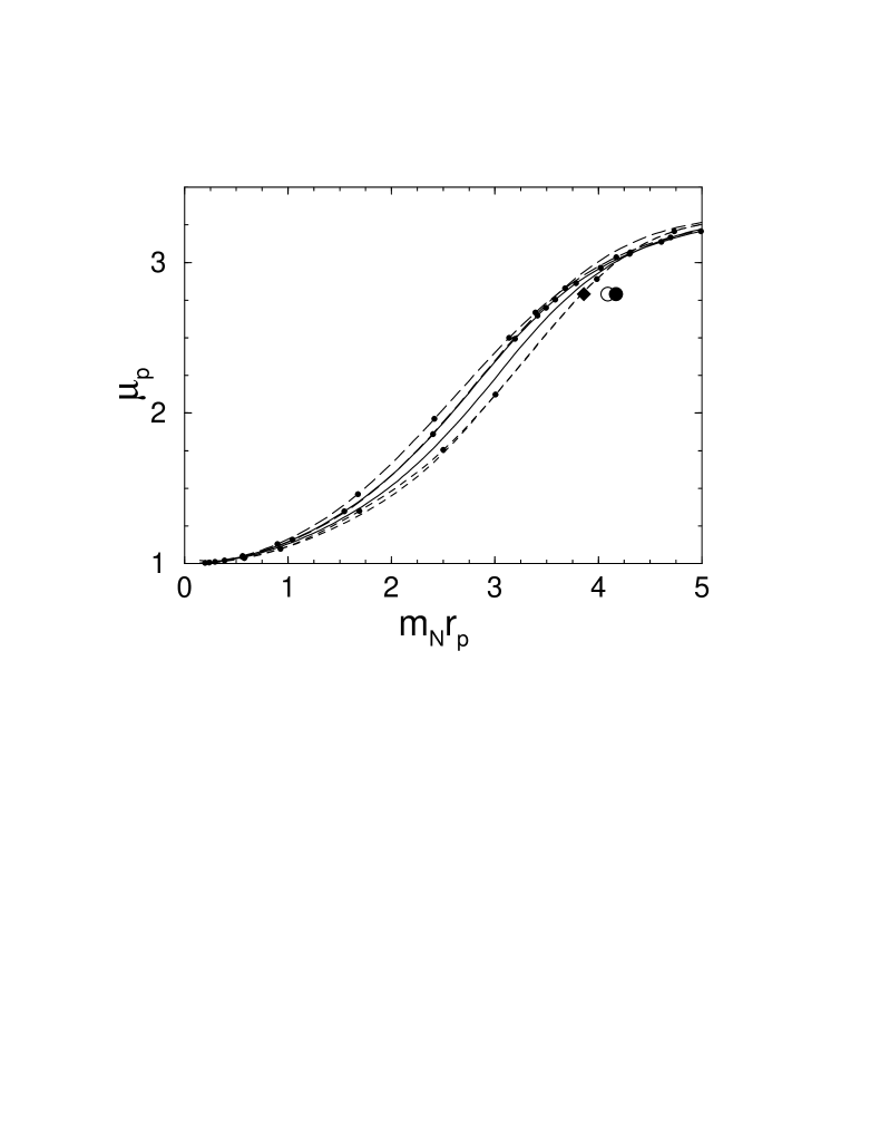
The functional dependence of the proton magnetic moment on the dimensionless product of nucleon mass and proton charge radius ($m_{N}r_{p}$) is shown in Figure 4. We basically reproduce the results previously found within the Bakamjian-Thomas spin coupling scheme[3]. We note that Ref.[3] used a proton radius given by the slope of the Dirac form factor $F_{1}(Q^{2})$. For the different spin coupling schemes there is a weak dependence of $\mu_{p}$ on the shape of the momentum wave function and moreover the dependence on different $\alpha$’s is small.

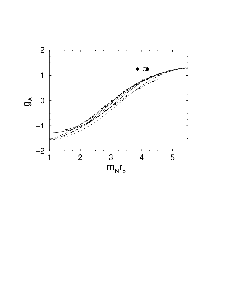
The weak isovector axial vector coupling constant $g_{A}$ as a function of the neutron magnetic moment is shown in Figure 5. Our calculations for $\alpha=1/2$ and harmonic oscillator wave function are in complete agreement with those of Konen and Weber[14], see Table III. The dependence on the shape of the momentum wave function is weak while increasing the constituent mass would allow us to achieve an agreement of the scalar quark coupling and the experimental data. The effective Lagrangian for the quark-nucleon coupling leads to an axial vector coupling constant that changes sign in the limit of a pointlike nucleon. This feature is not present in the Bakamjian-Thomas construction[3] as discussed in the previous section. In the limit $\beta\rightarrow 0$ the results for $g_{A}$ tend to the nonrelativistic value of 5/3 and in the limit of $\beta\rightarrow\infty$ corresponding to $\mu_{n}\rightarrow 0$ the axial coupling $g_{A}$ tends to $\approx-5/3$.

While the change in $\alpha$ has a considerable effect on $g_{A}$ for a given neutron magnetic moment (see Fig. 5) this behavior is not seen for $g_{A}$ as a function of the proton magnetic moment shown in Figure 6. The momentum shape of the wave function and different values of $\alpha$ produce small effects on the function $g_{A}(\mu_{p})$. Only the constituent mass can considerably shift the curve and from Table III we conclude that the experimental point can be reached with a mass of about 1/3 of the nucleon mass. However, the simultaneous fit of $\mu_{p}$, $\mu_{n}$ and $g_{A}$ for $\alpha=1$ seems difficult without invoking further physical aspects of the constituent quarks.

In Figure 7 the function defined by $g_{A}(m_{n}r_{p})$ has a weak dependence on momentum wave function form and spin coupling schemes. This result could be anticipated from the strong correlations of $g_{A}(\mu_{p})$ and $\mu_{p}(m_{n}r_{p})$ shown in Figures 6 and 4, respectively. The experimental point could be fitted by the increase of the constituent mass.

From the results shown in Figures 2 to 7 we conclude that without invoking more physics than is contained in the present model, each set of static observables either $\{r_{n},r_{p},\mu_{p},g_{A}\}$ or $\{r_{n},\mu_{n},g_{A}\}$ can be reasonably fitted to the experimental values with only two parameters, i.e. the width of the wave function and the constituent quark mass. The difficulty is related to the precise and simultaneous fit of the magnetic moments as shown in Figure 3.

B Nucleon Form Factors

In Figures 8 to 13 we show different electromagnetic and weak form factors as a function of $q^{2}$. We give results with the parameters of the Gaussian and power-law wave functions as given in Table I. For each $\alpha$ they are fitted to the neutron magnetic moment.

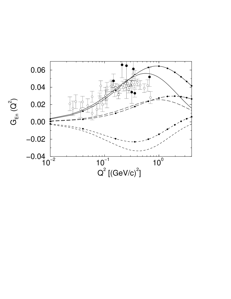
The neutron charge form factor is shown in Figure 8. The gradient spin coupling gives a negative contribution for $-q^{2}\lesssim 2$ (GeV/c)². The calculation for the mixed case ($\alpha=1/2$) underestimates the data. For the scalar quark spin coupling both types of momentum wave functions give results close to each other and within the experimental uncertainty agree with the data. For momentum transfers above 1 GeV/c, the model dependence (Power vs. HO) starts to appear in the neutron charge form factor.

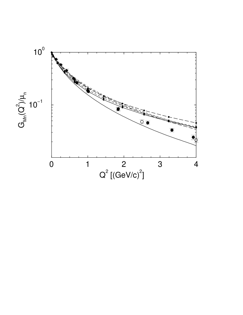
The theoretical results for $G_{Mn}(q^{2})$ are compared to the experiments in Figure 9. The calculations with scalar coupling between the quark pair ($\alpha=1$) give the best agreement with the data for both momentum wave function models. The results for $\alpha=0$ and 1/2 overestimate the data. For $-q^{2}\gtrsim 1$ (GeV/c)² the models deviate from experiments.

In Figure 10 we show the proton charge form factor compared with experiments. A common behavior is found for the calculations with both wave function models, i.e., the choice of $\alpha=1$ gives values below the experimental data. This could also be anticipated from Figures 3 and 4 that show too big values of the proton radius for $\mu_{n}=-1.91\mu_{N}$. The spin couplings given by $\alpha=0$ and 1/2 approach the data for $-q^{2}\lesssim 2$ (GeV/c)², because the proton radius is in better agreement with the experimental values.

In Figure 11 the results for the proton magnetic form factor are shown. The scalar quark spin coupling results approach experimental data for momentum transfers below 1 GeV/c and for both wave function models. The results obtained with the spin coupling parameterized by $\alpha=0$ and 1/2 overestimate the data.

In Figure 12 the results of recent measurements of the ratio $\mu_{p}G_{Ep}/G_{Mn}$ [27] are compared to our calculations. We observe a dependence on different spin couplings and momentum wave functions. However the data are generally underestimated that indicates the necessity for more sophisticated wave function models, inclusion of other spin couplings, and/or a constituent quark substructure. Let us emphasize that relativistic effects are crucial for the steeper proton charge form factor fall-off.

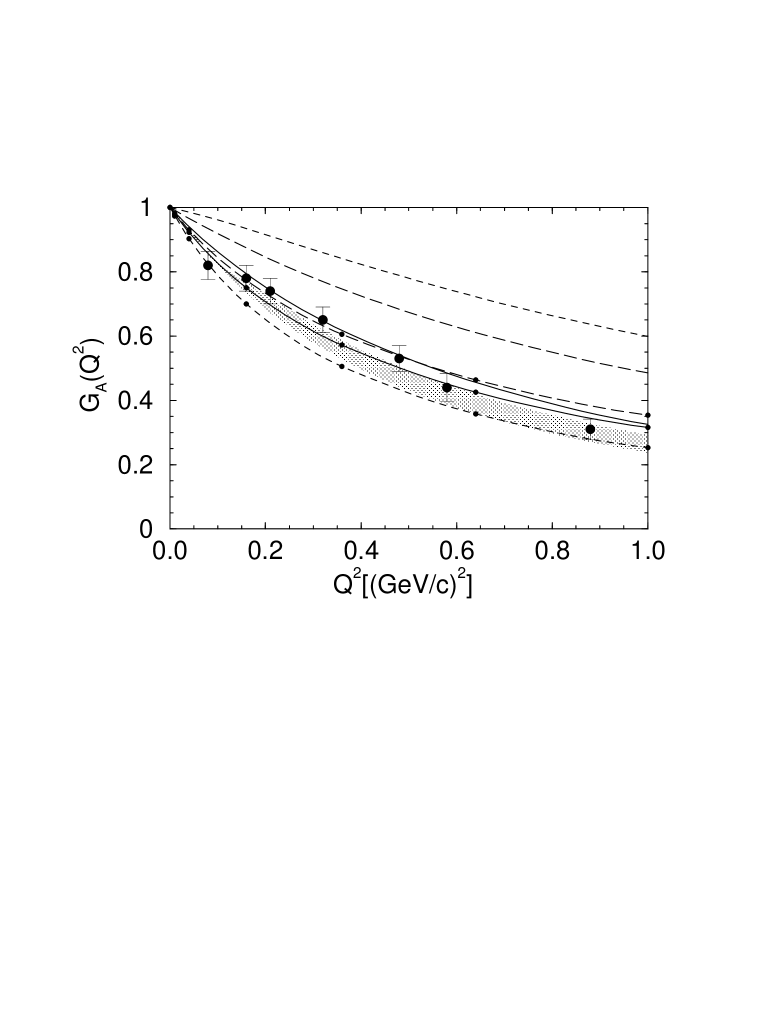
Finally, in Figure 13 the model results are compared to experimental data for the nucleon weak isovector axial vector form factor. The calculations with the scalar coupling between the quark pair produce the best agreement with the data. However a remarkable sensitivity to the coupling schemes and wave functions models is also seen in Figure 13. The model dependence found in this figure can be qualitatively understood if one looks at the approximate equation (63) for $g_{A}$, where a cancellation between two terms occurs that causes a high sensitivity to details of the models. This could also be expected for $q^{2}$-dependence of the axial vector form factor.

We must keep in mind that our wave function models are quite simplistic and even in the nonrelativistic quark model the nucleon is highly relativistic and the real wave function can strongly differ from their nonrelativistic counterparts. In this sense, the difference between the data and the present models seen in Figures 9 to 13 for momentum transfers of several GeV/c is not too serious considering the simplicity of the model. We should also mention that the concept of constituent quarks is expected to break down above the chiral symmetry breaking scale ($4\pi f_{\pi}\sim 1$ GeV), so that we expect the model to loose validity because current quarks become the relevant degrees of freedom revealing the constituent substructure.

V Summary and Conclusion

We have shown the effects of different forms of relativistic spin couplings of constituent quarks on the nucleon electroweak properties. Model independent (i.e. independent of the momentum shape of the light-front wave function) relations between the static electroweak observables are verified to hold within each quark spin coupling scheme as could be expected as $q^{2}\rightarrow 0$. It is found that, while the neutron charge form factor is very sensitive to different choices of spin coupling schemes, it is insensitive to the details of the momentum part of the three-quark wave function model for momentum transfers below 1 GeV/c. The experimental data on the neutron charge form factor – for momentum transfers below 1 GeV/c – can be reproduced by models with a scalar coupling of the constituent quark pair, independent of the shape of the wave function. This is mostly due to the momentum dependence in lower component of the quark spinors that leads to a mixed-symmetry space part (in a nonrelativistic reduction), compare also Ref. [30]. This feature is strongly suppressed in the mixed case ($\alpha=1/2$) and comes with an opposite sign for the pure scalar and pure gradient cases, respectively.

The difference between Bakamjian-Thomas and effective Lagrangian spin coupling schemes is particularly noticeable in the weak isovector axial vector coupling constant evaluated in the pointlike nucleon limit. The correlations involving the set of static observables $\{r_{p},\mu_{p},g_{A}\}$ are not very sensitive to spin coupling schemes defined by the effective Lagrangian for different values of $\alpha$ in Eq.(1). Among these relations, the function $g_{A}(\mu_{p})$ is shown to have the smallest dependence on spin coupling schemes and on the shape of the momentum wave function. The correlations involving the neutron magnetic moment are more sensitive to different spin coupling schemes. Overall, for momentum transfers above 1 GeV/c, we observe a dependence on the different spin coupling schemes and momentum wave functions. The new data on the ratio of $\mu_{p}G_{Ep}/G_{Mp}$ indicates the necessity to improve the wave function models, include other (e.g. axial-vector quark pair) spin coupling, and/or a description of constituent quarks beyond the models discussed in the present work. The influence of pionic corrections in a light front frame work has been studied in  [31]. From their results we expect that our conclusions do not change drastically, however, a complete study of pionic corrections in the present framework is still an open and challenging problem.

Acknowledgments: MB thanks R. Tegen for a discussion on $g_{A}$. HJW and MB thank the University of Virginia’s INPP for partial support. MB thanks the Deutscher Akademischer Austauschdienst (DAAD) and FAPESP for support, and the Department of Physics of ITA for the warm hospitality and for local support. WRBA thanks CNPq for financial support and LCCA/USP for providing computational facilities, EFS thanks FAPESP for financial support and TF thanks CNPq and FAPESP.

TABLE I.: Parameters for the HO $(\beta_{G})$ and power-law $(\beta_{P})$ models of the nucleon momentum wave function with different spin coupling schemes from the fit of $\mu_{n}=-1.91\mu_{\rm N}$ with $m=$ 220 MeV.

$\alpha$	$\beta_{G}$[MeV]	$\beta_{P}$ [MeV]
1	562	477
1/2	664	576
0	661	411

TABLE II.: Values for $\xi(0)$ from the different models (HO, Power) using the parameters of Table I, $\xi^{\mathrm{expt.}}=0.21\pm 0.08$.

$\alpha$	$\xi_{G}(0)$	$\xi_{P}(0)$
1	0.54	0.69
1/2	1.6	1.6
0	3.0	2.6

TABLE III.: Nucleon low-energy electroweak observables for different spin coupling parameters with a gaussian light-front wave function for $m$=330, 360 and 380 MeV with the values of $\beta$ parameter from Konen and Weber[14] (in their work the Gaussian parameter is $\beta/\sqrt{3}$ ).

$m$[MeV]	$\alpha$	$r^{2}_{En}$ [fm2]	$r^{2}_{Ep}$ [fm2]	$\mu_{n}[\mu_{\rm N}]$	$\mu_{p}[\mu_{\rm N}]$	$g_{A}$
	0	0.035	0.69	-1.83	2.84	1.09
330	1/2	-0.024	0.69	-1.73	2.80	1.20
	1	-0.080	0.71	-1.60	2.71	1.25
	0	0.023	0.66	-1.77	2.77	1.13
360	1/2	-0.025	0.66	-1.67	2.72	1.23
	1	-0.073	0.67	-1.53	2.62	1.29
	0	0.018	0.62	-1.71	2.72	1.19
380	1/2	-0.027	0.62	-1.61	2.66	1.20
	1	-0.071	0.63	-1.47	2.56	1.29
			0.66 $\pm$ 0.06[16],
EXP.		-0.113 $\pm$ 0.005[15]	0.74 $\pm$ 0.02[17],	-1.91	2.79	1.2670 $\pm$ 0.0035 [19]
			0.77 $\pm$ 0.03[18]

 

FIG. 1.: Feynman diagrams for the nucleon electroweak current. The gray blob represents the spin invariant for the coupled quark pair in the effective Lagrangian, Eq.(1). The black circle in the fermion line represents the action of the current operator on the quark. The current operator can represent either the electromagnetic current or the weak isovector axial vector current. Diagram (1a) represents either $J^{+}_{aN}$, Eq.(18), or $A^{+}_{aN}$, Eq.(41). Diagram (1b) represents either $J^{+}_{bN}$, Eq.(20), or $A^{+}_{bN}$, Eq.(43). Diagram (1c) represents either $J^{+}_{cN}$, Eq.(22), or $A^{+}_{cN}$, Eq.(45). Diagram (1d) represents $J^{+}_{dN}$, Eq.(24). Diagram (1d) does not contribute to the weak isovector axial vector current due to the isoscalar nature of the coupled quark pair.

FIG. 2.: Neutron charge square radius as a function of the neutron magnetic moment. Results for the Gaussian wave function with $\alpha$ equal to 1 (solid line), 1/2 (dashed line) and 0 (short-dashed line). Results for the power-law wave function with $\alpha$ equal to 1 (solid line with dots), 1/2 (dashed line with dots) and 0 (short-dashed line with dots). Experimental data from Ref.[15].

FIG. 3.: Proton magnetic moment as a function of the neutron magnetic moment. Theoretical curves labeled as in Fig.2. The experimental data are represented by the full circle.

FIG. 4.: Proton magnetic moment as a function of the dimensionless product $m_{N}r_{p}$. Theoretical curves labeled as in Fig.2. Experimental points are given by a full diamond[16], open circle[17] and full circle[18].

FIG. 5.: Nucleon axial vector coupling constant as a function of the neutron magnetic moment. Theoretical curves labeled as in Fig.2. The experimental point is given by the full circle.

FIG. 6.: Nucleon axial vector coupling constant as a function of the proton magnetic moment. Theoretical curves labeled as in Fig.2. The experimental point given by the full circle.

FIG. 7.: Nucleon axial vector coupling constant as a function of the dimensionless product of the proton charge radius and mass. Theoretical curves labeled as in Fig.2. Experimental points are given by a full diamond[16], open circle[17] and full circle[18].

FIG. 8.: Neutron charge form factor as a function of the momentum transfer $q^{2}=-Q^{2}$. Theoretical curves labeled as in Fig.2. The empty circles are the experimental data from Ref.[20] and the full circles from Ref.[21].

FIG. 9.: Neutron magnetic form factor $G_{Mn}/\mu_{n}$ as a function of momentum transfer squared. Theoretical curves labeled as in Fig.2. The experimental data come from Ref.[22], full circles; Ref.[23], open circles; Ref.[24], full diamonds.

FIG. 10.: Proton charge form factor as a function of momentum transfer squared. Theoretical curves labeled as in Fig. 2. The experimental data come from Ref.[25].

FIG. 11.: Proton magnetic form factor $G_{Mp}/\mu_{p}$ as a function of momentum transfer squared. Theoretical curves labeled as in Fig. 2. The experimental data come from Ref.[26].

FIG. 12.: Proton form factor ratio $\mu_{p}G_{Ep}/G_{Mp}$ as a function of momentum transfer squared. Theoretical curves labeled as in Fig. 2. The experimental data come from Ref.[27].

FIG. 13.: Normalized axial vector form factor as a function of momentum transfer squared. Theoretical curves labeled as in Fig. 2. The experimental data come from Ref.[28]. The experimental data of Ref.[29] are given in terms of a dipole form with a combined fit of $m_{A}=1.03\pm 0.05$ GeV.

REFERENCES

[1] W.R.B. de Araújo, E.F. Suisso, T.Frederico,
M.Beyer and H.J. Weber, Phys. Lett. B478 (2000) 86.
[2] J. Carbonell, B. Desplanques, V. Karmanov and
J.-F. Mathiot, Phys. Reports 300 (1998) 215 , and references
therein.
[3]S.J. Brodsky and F.Schlumpf, Phys. Lett. B329 (1994)111;
Prog.Part. Nucl.Phys. 34 (1995)69.
[4]S.J. Brodsky, H.-C. Pauli and S.S.Pinsky, Phys. Rep.
301 (1998)299.
[5] M. R. Frank, B. K. Jennings and G. A. Miller,
Nucleonic Wave Functions,”
Phys. Rev. C54, 920 (1996)
[6] T. Frederico and G.A. Miller, Phys. Rev. D45 (1992) 4207.
[7]J.P.B.C de Melo, H.W. Naus and T. Frederico,
Phys. Rev. C59 (1999) 2278.
[8] J.P.B.C. de Melo and T. Frederico,
Phys. Rev. C55 (1997) 2043, and references therein.
[9]W.R.B. de Araújo, M. Beyer, T. Frederico and H.J. Weber,
J. Phys. G 25 (1999) 158.
[10] M. Beyer, C. Kuhrts, and H. J. Weber, Ann. Phys. (NY)
269 (1998) 129, and references therein.
[11] B. Bakamjian and L. H. Thomas, Phys. Rev. 92
(1953) 1300.
[12]F. Cardarelli, E. Pace, G. Salme and S. Simula,
Phys. Lett. B357 (1995) 267; Few Body Syst. Suppl. 8 (1995) 345;
F. Cardarelli and S. Simula, Phys. Lett. B467 (1999) 1; ibidem,
nucl-th/0006023.
[13] R. Tegen, Phys. Rev. Lett. 62 (1989) 1724.
[14] W.Konen and H.J. Weber, Phys. Rev. D41 (1991) 2201.
[15] S. Kopecky et al., Phys. Rev. Lett. 74 (1995) 2427.
[16] S.J. Brodsky and J.R. Primack, Ann. Phys. (N.Y.) 52
(1969) 315.
[17] J.J. Murphy II, Y.M. Shin, and D.M. Skopik, Phys. Rev.
C9 (1974) 3125.
[18] R. Rosenfelder, Phys. Lett. B479(2000)381.
[19] D.E. Groom et al., The European Physics Journal
15 (2000) 1.
[20] S.Platchkov et al., Nucl.Phys. A510 (1990) 740.
[21] T. Eden et al., Phys. Rev. C50 (1994) R1749;
M. Meyerhoff et al., Phys. Lett. B327 (1994) 201; C. Herberg et al.,
Eur. Phys. J. A5 (1999) 131; I. Passchier et al., Phys. Rev. Lett.
82 (1999) 4988; M. Ostrick et al., Phys. Rev. Lett. 83 (1999) 276;
G. Becker et al. submitted to Eur. Phys. J.
[22] W. Albrecht et al., Phys. Lett. B26 (1968) 642.
[23] S. Rock et al., Phys. Rev. Lett. 49 (1982) 1139.
[24] E.E.W. Bruins et al., Phys. Rev. Lett. (1995) 1.
[25] G. Hohler et al., Nucl. Phys. B144 (1976) 505.
[26] W. Bartel et al., Nucl. Phys. B58 (1973) 429.
[27] M.K. Jones et al., Phys. Rev. Lett. 84(2000)1398.
[28] A. Del Guerra et al., Nucl.Phys. B99 (1975) 253;
Nucl.Phys. B107 (1976) 65.
[29] N.J. Baker et al., Phys. Rev. D23 (1982) 2499;
S.V. Belikov et al., Z. Phys. A320 (1985) 625;
T. Kitagaki et al., Phys. Rev. D42 (1990) 1331.
[30]
F. Cardarelli and S. Simula,
Phys. Rev. C62, 065201 (2000).
[31]
Z. Dziembowski, H. Holtmann, A. Szczurek and J. Speth,
Annals Phys. 258 (1997) 1.
TABLE I.: Parameters for the HO and
power-law models of the nucleon momentum wave function
with different spin coupling schemes from the fit of with 220 MeV.
[MeV]
1
562
477
1/2
664
576
0
661
411
TABLE II.: Values for from the different models
(HO, Power) using the parameters of Table I,