Density dependent hadron field theory for asymmetric nuclear matter and exotic nuclei

Abstract

The density dependent relativistic hadron field (DDRH) theory is applied to strongly asymmetric nuclear matter and finite nuclei far off stability. A new set of in-medium meson-nucleon vertices is derived from Dirac-Brueckner Hartree-Fock (DBHF) calculations in asymmetric matter, now accounting also for the density dependence of isovector coupling constants. The scalar-isovector $\delta$ meson is included. Nuclear matter calculations show that it is necessary to introduce a momentum correction in the extraction of coupling constants from the DBHF self-energies in order to reproduce the DBHF equation of state by DDRH mean-field calculations. The properties of DDRH vertices derived from the Groningen and the Bonn A nucleon-nucleon (NN) potentials are compared in nuclear matter calculations and for finite nuclei. Relativistic Hartree results for binding energies, charge radii, separation energies and shell gaps for the Ni and Sn isotopic chains are presented. Using the momentum corrected vertices an overall agreement to data on a level of a few percent is obtained. In the accessible range of asymmetries the $\delta$ meson contributions to the self-energies are found to be of minor importance but asymmetry dependent fluctuations may occur.

I Introduction

The modern approach to nuclear structure is based on relativistic models describing nuclear matter and finite nuclei as a strongly interacting systems of baryons and mesons. Starting from a Lagrangian formulation a phenomenological hadronic field theory is obtained by adjusting the meson-nucleon coupling constants to various properties of infinite nuclear matter and finite nuclei [1, 2]. A connection to free space nucleon-nucleon interactions is not attempted. The prototype for such an approach is relativistic mean-field theory (RMF) [3, 4] where nuclear forces are obtained from the virtual exchange of mesons, finally leading to condensed classically fields produced by nucleonic sources. Using this procedure recent RMF models have been remarkably successful in describing nuclei over the entire range of the periodic table [5, 6, 7, 8, 9]. In order to improve results cubic and quartic self-interactions of the mesons fields had to be introduced [10, 11]. Although higher order scalar self-interactions can be motivated by vacuum renormalization [4] in practice the strengths of the self-couplings are determined in a purely phenomenological way. In mean-field approximation the mesonic self-interactions correspond effectively to higher order density dependent contributions. Using up to quartic terms a good description of nuclear matter and finite nuclei is obtained but, depending on the sign of especially the quartic scalar $\sigma$ self-interaction, instabilities occur in the region above saturation density [5].

A more fundamental - but also more elaborate - approach is to derive in-medium interactions microscopically. An appropriate and successful method is Dirac-Brueckner theory (DB). Using realistic NN potentials in-medium interactions are derived by a complete re-summation of (two-body) ladder diagrams. A break-through was obtained with relativistic Brueckner theory which reproduces the empirical saturation properties of nuclear matter reasonably well [12, 13, 14, 15, 16, 17, 18]. Since full-scale DB calculations for finite nuclei are not feasible a practical approach is to apply infinite matter DB results in local density approximation (LDA) to finite nuclei [19, 20, 21]. Retaining a Lagrangian formulation this is achieved by introducing density dependent meson-nucleon coupling constants taken from DB self-energies [19]. In [22, 23] it was pointed out that such an approach does not comply with relativity and thermodynamics. A fully covariant and thermodynamically consistent field theory, however, is obtained by treating the interaction vertices on the level of the Lagrangian as Lorentz-scalar functionals of the field operators. In the density dependent relativistic hadron field (DDRH) theory [22, 23] the medium dependence of the vertices is expressed by functionals of the baryon field operators. An important difference to the RMF treatment of non-linearities is that the DDRH approach accounts for quantal fluctuations of the baryon fields even in the ground state. Such effects contribute as rearrangement self-energies to the baryon field equations describing the static polarization of the background medium by a nucleon [23, 24]. Since DDRH theory provides a systematic expansion of interactions in terms of higher order baryon-baryon correlation functions [22, 23], extensions beyond the mean-level are in principle possible.

In mean-field approximation DDRH theory reduces to a Hartree description with density dependent coupling constants similar to the initial proposal of Brockmann and Toki [19]. The rearrangement contributions significantly improve the binding energies and radii of finite nuclei. Several calculations in the DDRH model for stable nuclei have been performed [23, 25, 26, 27] using density dependent vertices derived from DB calculations with the Bonn A potential [15, 28]. Recently, a phenomenological approach to DDRH theory was presented [29] by determining the density dependence of the vertices empirically. Descriptions of finite nuclei of a quality comparable to non-linear RMF models were obtained. Extensions to the baryon octet sector and hypernuclei are discussed in [30].

The main intention of this paper is to apply DDRH theory to asymmetric matter and nuclei far off stability. Since the vertex functionals used in the former applications were taken from DB calculations in symmetric matter, information on the density dependence of isovector vertices was not available. From the DB results for asymmetric matter, obtained in Ref. [18, 31] with the Groningen potential [32], a new set of coupling constants has been derived, now including density dependent isoscalar ($\sigma$, $\omega$) and isovector ($\delta$, $\rho$) vertices. Contributions from the scalar-isoscalar $\delta$ meson are of special interest at extreme neutron-to-proton ratios.

From inifinite matter calculations it was found that the momentum dependence of self-energies has to be taken into account in order to reproduce the underlying DBHF equation of state by DDRH calculations. In a strict sense this means to go beyond the static Hartree limit. A closer inspection, however, shows that for a mean-field description it is sufficient to account for the momentum dependence on an average level. Rather than using the self-energies at the Fermi-surface [15, 18] a more appropriate method is to extract coupling constants from self-energies averaged over the Fermi-sphere. This still leads to static vertices but incorporating momentum dependent corrections.

The paper is arranged as follows. In Sec. II the DDRH approach and the mean-field reduction are reviewed. In Sec. III the approach to extract density dependent coupling constants from nuclear matter DB self-energies including isovector contributions and the momentum corrections is presented. The global properties of the newly determined coupling constants are investigated in applications to infinite matter. In Sec. IV we report on DDRH calculations for the isotopic chains of Ni and Sn nuclides, both including stable and exotic nuclei. These two isotopic chains are of special interest because several magic neutron numbers and the corresponding shell closures are covered on top of the magic Z=28 and Z=50 proton numbers, respectively. Results for the Groningen and the Bonn A NN potentials are compared. Contribution from the scalar-isoscalar $\delta$ meson and the influence of the momentum correction are examined in detail. The paper closes in Sec. V with a summary and conclusions.

II Density dependent hadron field theory for asymmetric nuclear matter

II.1 The model Lagrangian and the equations of motion

The density dependent relativistic hadron field (DDRH) theory has been presented and thoroughly discussed in [22, 23, 30]. In this work we restrict ourselves to a short review of the model and to a discussion of the extensions to Ref. [23].

The model Lagrangian includes the baryons represented as Dirac spinors $\Psi=\left(\psi_{p},\psi_{n}\right)^{T}$, the isocalar mesons $\sigma$ and $\omega$, the isovector $\rho$ meson and the photon $\gamma$. In addition to former models we also include the scalar isovector meson $\delta$ which is important in asymmetric systems and naturally has to be taken into account when extracting the coupling functionals from asymmetric nuclear matter DBHF calculations as will be explained in detail later. The Lagrangian is

$${\mathcal{L}} = {\mathcal{L}}_{B}+{\mathcal{L}}_{M}+{\mathcal{L}}_{int}$$

$${\mathcal{L}}_{B} = \overline{\Psi}\left[i\gamma_{\mu}\partial^{\mu}-M\right]\Psi$$ (1)

$${\mathcal{L}}_{M} = \frac{1}{2}\sum_{i=\sigma,\delta}\left(\partial_{\mu}\Phi_{i}\partial^{\mu}\Phi_{i}-m_{i}^{2}\Phi_{i}^{2}\right)-$$ (2)

$$\frac{1}{2}\sum_{\kappa=\omega,\rho,\gamma}\left(\frac{1}{2}F^{(\kappa)}_{\mu\nu}F^{(\kappa)\mu\nu}-m_{\kappa}^{2}A^{(\kappa)}_{\mu}A^{(\kappa)\mu}\right)$$

$${\mathcal{L}}_{int} = \overline{\Psi}\hat{\Gamma}_{\sigma}(\overline{\Psi},\Psi)\Psi\Phi_{\sigma}-\overline{\Psi}\hat{\Gamma}_{\omega}(\overline{\Psi},\Psi)\gamma_{\mu}\Psi A^{(\omega)\mu}+$$ (3)

$$\overline{\Psi}\hat{\Gamma}_{\delta}(\overline{\Psi},\Psi)\bm{\tau}\Psi\bm{\Phi}_{\delta}-\overline{\Psi}\hat{\Gamma}_{\rho}(\overline{\Psi},\Psi)\gamma_{\mu}\bm{\tau}\Psi\bm{A}^{(\rho)\mu}-$$

$$e\overline{\Psi}\hat{Q}\gamma_{\mu}\Psi A^{(\gamma)\mu}.$$

Here, ${\mathcal{L}}_{B}$ and ${\mathcal{L}}_{M}$ are the free baryonic and the free mesonic Lagrangians, respectively, and interactions are described by ${\mathcal{L}}_{int}$, where

$$F^{(\kappa)}_{\mu\nu}=\partial_{\mu}A_{\nu}^{(\kappa)}-\partial_{\nu}A_{\mu}^{(\kappa)}$$ (4)

is the field strength tensor of either the vector mesons ($\kappa=\omega,\rho$) or the photon ($\kappa=\gamma$) and $\hat{Q}$ is the electric charge operator.

The main difference to standard QHD models [3, 4] is that the meson-baryon vertices $\hat{\Gamma}_{\alpha}$ ($\alpha=\sigma,\omega,\delta,\rho$) are not constant numbers but depend on the baryon field operators $\Psi$. Relativistic covariance requires that the vertices are functions $\hat{\Gamma}_{\alpha}(\hat{\rho})$ of Lorenz-scalar bilinear forms $\hat{\rho}(\overline{\Psi},\Psi)$ of the field operators. Two obvious choices are the scalar density dependence (SDD) with $\hat{\rho}=\overline{\Psi}\Psi$ and the vector density dependence (VDD) where $\hat{\rho}^{2}=\hat{j}_{\mu}\hat{j}^{\mu}$ depends on the square of the baryon vector current $\hat{j}_{\mu}=\overline{\Psi}\gamma_{\mu}\Psi$. In this work we only present results for the VDD description since it leads to better results for finite nuclei [23] and gives a more natural connection to the parameterization of the DB vertices. This will be discussed in detail in the next section.

As pointed out in [23] the most important difference to RMF [2] or convential DD [19] theories is the contribution from the rearrangement self-energies to the DDRH baryon field equations. This is evident since the variational derivative of ${\mathcal{L}}_{int}$ with respect to $\overline{\Psi}$ will also act on the vertices.

$$\frac{\delta{\mathcal{L}}_{int}}{\delta\overline{\Psi}}=\frac{\partial{\mathcal{L}}_{int}}{\partial\overline{\Psi}}+\frac{\partial{\mathcal{L}}_{int}}{\partial\hat{\rho}}\frac{\delta\hat{\rho}}{\delta\overline{\Psi}}$$ (5)

The second term on the right hand side of the equation is the rearrangement contribution to the self-energy. Rearrangement accounts physically for static polarization effects in the nuclear medium, cancelling certain classes of particle-hole diagrams [24]. The usual self-energies are defined as

$$\hat{\Sigma}^{s(0)} = \hat{\Gamma}_{\sigma}(\hat{\rho})\Phi_{\sigma}+\hat{\Gamma}_{\delta}(\hat{\rho})\bm{\tau}\bm{\Phi}_{\delta}$$ (6)

$$\hat{\Sigma}^{\mu(0)} = \hat{\Gamma}_{\omega}(\hat{\rho})A^{(\omega)\mu}+\hat{\Gamma}_{\rho}(\hat{\rho})\bm{\tau}\bm{A}^{(\rho)\mu}+e\hat{Q}A^{(\gamma)\mu}.$$ (7)

while the vector rearrangement self-energies are obtained from Eq. (5) as

$$\hat{\Sigma}^{\mu(r)} = \left(\frac{\partial\hat{\Gamma}{{}_{\omega}}}{\partial\hat{\rho}}A^{(\omega)\nu}\hat{j}_{\nu}+\frac{\partial\hat{\Gamma}{{}_{\rho}}}{\partial\hat{\rho}}\bm{\tau}\bm{A}^{(\rho)\nu}\hat{j}_{\nu}\right.$$ (8)

$$- \left.\frac{\partial\hat{\Gamma}{{}_{\sigma}}}{\partial\hat{\rho}}\Phi_{\sigma}\overline{\Psi}\Psi-\frac{\partial\hat{\Gamma}{{}_{\delta}}}{\partial\hat{\rho}}\bm{\tau}\bm{\Phi}_{\delta}\overline{\Psi}\Psi\right)\hat{u}^{\mu}.$$

Here, $\hat{u}^{\mu}$ is a four velocity with $\hat{u}^{\mu}\hat{u}_{\mu}=1$. Defining

$$\hat{\Sigma}^{s}=\hat{\Sigma}^{s(0)},\quad\hat{\Sigma}^{\mu}=\hat{\Sigma}^{\mu(0)}+\hat{\Sigma}^{\mu(r)}$$ (9)

the structure of the baryon field equations takes on the standard form

$$\left[\gamma_{\mu}\left(i\partial^{\mu}-\hat{\Sigma}^{\mu}\right)-\left(M-\hat{\Sigma}^{s}\right)\right]\Psi=0,$$ (10)

however, the underlying dynamics is changed by the rearrangement contributions. In addition the effective baryon mass $M^{*}=M-\hat{\Sigma}^{s}$ differs for protons and neutrons due to the inclusion of the scalar isovector $\delta$ meson. This is an additional property of the model that was not present in the previous formulation [22, 23] where only the $\rho$ meson in the isovector part of the interaction was considered. We also find that the density dependence of the $\rho$ and $\delta$ mesons gives an additional contribution to the vector rearrangement self-energies.

II.2 Mean-field reduction

The field equations are solved in the Hartree mean-field approximation. In the Hartree approach the highly complex form of the vertex functionals and its derivatives can be treated in a simple way using Wick’s theorem [33]. Calculating the expectation value with respect to the ground state $|0\rangle$ the vertices reduce to

$$\langle\hat{\Gamma}_{\alpha}(\hat{\rho})\rangle=\Gamma_{\alpha}(\langle\hat{\rho}\rangle)=\Gamma_{\alpha}(\rho)$$ (11)

and

$$\left<\frac{\partial\hat{\Gamma}_{\alpha}(\hat{\rho})}{\partial\hat{\rho}}\right>=\frac{\partial\Gamma_{\alpha}(\rho)}{\partial\rho}.$$ (12)

where in the VDD case $\langle\hat{\rho}\rangle=\rho$ is just the baryon ground state density.

Meson fields are treated as static classical fields, time reversal symmetry is assumed, therefore only the zero component of the vector fields contributes. The meson field equations reduce to

$$(-\bm{\nabla}^{2}+m_{\sigma}^{2})\Phi_{\sigma} = \Gamma_{\sigma}(\rho)\rho^{s}$$ (13)

$$(-\bm{\nabla}^{2}+m_{\omega}^{2})A^{(\omega)}_{0} = \Gamma_{\omega}(\rho)\rho$$ (14)

$$(-\bm{\nabla}^{2}+m_{\delta}^{2})\Phi_{\delta} = \Gamma_{\delta}(\rho)\rho^{s}_{3}$$ (15)

$$(-\bm{\nabla}^{2}+m_{\rho}^{2})A^{(\rho)}_{0} = \Gamma_{\rho}(\rho)\rho_{3}$$ (16)

$$-\bm{\nabla}^{2}A^{(\gamma)}_{0} = -e\rho_{p}$$ (17)

where the densities are the following ground state expectation values

$$\rho^{s}=\langle\overline{\Psi}\Psi\rangle = \rho_{n}^{s}+\rho_{p}^{s}$$ (18)

$$\rho=\langle\overline{\Psi}\gamma_{0}\Psi\rangle = \rho_{n}+\rho_{p}$$ (19)

$$\rho_{3}^{s}=\langle\overline{\Psi}\tau_{3}\Psi\rangle = \rho_{n}^{s}-\rho_{p}^{s}$$ (20)

$$\rho_{3}=\langle\overline{\Psi}\gamma_{0}\tau_{3}\Psi\rangle = \rho_{n}-\rho_{p}$$ (21)

and the indices $n$ and $p$ stand for neutrons and protons, respectively. We will use the index $b=n,p$ to distinguisch between different nucleons.

The Dirac equation, separated in isospin, is the only remaining operator field equation

$$\left[\gamma_{\mu}\left(i\partial^{\mu}-\Sigma_{b}^{\mu}(\rho)\right)-\left(M-\Sigma_{b}^{s}(\rho)\right)\right]\psi_{b}=0$$ (22)

and contains now the static density dependent self energies

$$\Sigma_{b}^{s(0)}(\rho) = \Gamma_{\sigma}(\rho)\Phi_{\sigma}+\tau_{b}\Gamma_{\delta}(\rho)\Phi_{\delta}$$ (23)

$$\Sigma_{b}^{0(0)}(\rho) = \Gamma_{\omega}(\rho)A_{0}^{(\omega)}+\tau_{b}\Gamma_{\rho}(\rho)A_{0}^{(\rho)}+e\frac{1-\tau_{b}}{2}A_{0}^{(\gamma)}$$ (24)

$$\Sigma^{0(r)}(\rho) = \left(\frac{\partial\Gamma{{}_{\omega}}}{\partial\rho}A_{0}^{(\omega)}\rho+\frac{\partial\Gamma{{}_{\rho}}}{\partial\rho}A_{0}^{(\rho)}\rho_{3}\right.$$ (25)

$$- \left.\frac{\partial\Gamma{{}_{\sigma}}}{\partial\rho}\Phi_{\sigma}\rho^{s}-\frac{\partial\Gamma{{}_{\delta}}}{\partial\rho}\Phi_{\delta}\rho^{s}_{3}\right).$$

The self-energies differ for protons and neutrons ($\tau_{n}=+1$, $\tau_{p}=-1$) while the rearrangement self-energies are independent of the isospin.

III Relativistic Hartree description of infinite nuclear matter

III.1 Properties of infinite nuclear matter

In nuclear matter the field equations further simplify assuming translational invariance and neglecting the electromagnetic field. Solutions of the stationary Dirac equation

$$\left[\gamma_{\mu}k_{b}^{*\mu}-m_{b}^{*}\right]u_{b}^{*}(k)=0$$ (26)

are the usual plane wave Dirac spinors [34]

$$u^{*}_{b}(k)=\sqrt{\frac{E^{*}_{b}+m^{*}_{b}}{2m^{*}_{b}}}\left(\begin{array}[]{c}1\\ \frac{\bm{\sigma}\bm{k}^{*}_{b}}{E^{*}_{b}+m^{*}_{b}}\end{array}\right)\chi_{b}$$ (27)

where $\chi_{b}$ is a two-component Pauli spinor and the index $b$ distinguishes between neutrons and protons. The effective mass $m^{*}_{b}=M-\Sigma_{b}^{s}$ differs for neutrons and protons due to the inclusion of the $\delta$ meson in the scalar self-energy. The kinetic 4-momenta $k_{b}^{*\mu}=k_{b}^{\mu}-\Sigma_{b}^{\mu}$ and the energy $E_{b}^{*}$ of the particle are related by the in-medium on-shell condition ${k_{b}^{*}}^{2}={m_{b}^{*}}^{2}$ leading to $E^{*}_{b}={(k_{b}^{*0})}^{2}=\sqrt{{\bm{k}^{*}_{b}}^{2}+{m^{*}_{b}}^{2}}$. Integrating over all states $k\leq k_{F_{b}}$ inside the Fermi sphere and introducing $E_{F_{b}}=\sqrt{k_{F_{b}}^{2}+{m_{b}^{*}}^{2}}$ the scalar and vector densities in infinite nuclear matter are found as

$$\rho_{b} = \frac{2}{(2\pi)^{3}}\int_{|k|<k_{F_{b}}}d^{3}k=\frac{k_{F_{b}}^{3}}{3\pi^{2}}$$ (28)

$$\rho_{b}^{s} = \frac{2}{(2\pi)^{3}}\int_{|k|<k_{F_{b}}}d^{3}k\frac{m_{b}^{*}}{E_{b}^{*}}$$ (29)

$$= \frac{m_{b}^{*}}{2\pi^{2}}\left[k_{F_{b}}E_{F_{b}}+{m_{b}^{*}}^{2}\ln\frac{k_{F_{b}}+E_{F_{b}}}{m_{b}^{*}}\right].$$

Calculation of the energy density and the pressure from the energy-momentum tensor

$$T^{\mu\nu}=\sum_{i}\frac{\partial{\mathcal{L}}}{\partial(\partial_{\mu}\phi_{i})}\partial^{\nu}\phi_{i}-g^{\mu\nu}{\mathcal{L}}$$ (30)

$$\phi_{i}=\overline{\Psi},\Psi,\Phi_{\sigma},A^{(\omega)}_{\mu},\Phi_{\delta},A^{(\rho)}_{\mu}$$

is straightforward and the results are obtained in closed form

$$\epsilon=\langle T^{00}\rangle = \sum_{b=n,p}\frac{1}{4}\left[3E_{F_{b}}\rho_{b}+m_{b}^{*}\rho_{b}^{s}\right]$$ (31)

$$+ \frac{1}{2}\left[m_{\sigma}^{2}\Phi_{\sigma}^{2}+m_{\delta}^{2}\Phi_{\delta}^{2}+m_{\omega}^{2}{A^{(\omega)}_{0}}^{2}+m_{\rho}^{2}{A^{(\rho)}_{0}}^{2}\right]$$

$$= \sum_{b=n,p}\frac{1}{4}\left[3E_{F_{b}}\rho_{b}+m_{b}^{*}\rho_{b}^{s}\right]$$

$$+ \sum_{b=n,p}\frac{1}{2}\left[\rho_{b}\Sigma_{b}^{0(0)}+\rho_{b}^{s}\Sigma_{b}^{s(0)}\right]$$

$$p=\frac{1}{3}\sum_{i=1}^{3}\langle T^{ii}\rangle = \sum_{b=n,p}\frac{1}{4}\left[E_{F_{b}}\rho_{b}-m_{b}^{*}\rho_{b}^{s}\right]+\sum_{b=n,p}\rho_{b}\Sigma^{0(r)}$$ (32)

$$- \frac{1}{2}\left[m_{\sigma}^{2}\Phi_{\sigma}^{2}+m_{\delta}^{2}\Phi_{\delta}^{2}-m_{\omega}^{2}{A^{(\omega)}_{0}}^{2}-m_{\rho}^{2}{A^{(\rho)}_{0}}^{2}\right]$$

$$= \sum_{b=n,p}\frac{1}{4}\left[E_{F_{b}}\rho_{b}-m_{b}^{*}\rho_{b}^{s}\right]+\rho\Sigma^{0(r)}$$

$$+ \sum_{b=n,p}\frac{1}{2}\left[\rho_{b}\Sigma_{b}^{0(0)}-\rho_{b}^{s}\Sigma_{b}^{s(0)}\right]$$

From these relations it is seen that rearrangement does not affect the energy density but contributes explicitly to the pressure $p$. It is obvious from this that not taking into account rearrangement would violate thermodynamical consistency because the mechanical pressure $p$ obtained from the energy-momentum tensor must coincide with the thermodynamical derivation

$$p_{\text{thermo}}=\rho^{2}\frac{\partial}{\partial\rho}\left(\frac{\epsilon}{\rho}\right)=p.$$ (33)

III.2 Nucleon-meson vertices from Dirac-Brueckner theory and the momentum correction

Since the DDRH nucleon-meson vertices are deduced from microscopic Dirac-Brueckner calculations the question arises about the best ansatz for the extraction of the DB results. This has been discussed extensively in [30]. For a given infinite nuclear matter DB vertex $\Gamma_{\alpha}(\rho_{nm})$ the mapping to the field theoretical formulation is defined by [23]

$$\Gamma_{\alpha}(\hat{\rho})=\int_{0}^{\infty}\Gamma_{\alpha}(\rho_{nm})\delta(\rho_{nm}^{2}-\hat{\rho}^{2})2\rho_{nm}d\rho_{nm}$$ (34)

and directly allows us to apply the DB results to our model. Still, we have not defined how to extract the DB vertices $\Gamma_{\alpha}(\rho_{nm})$ at a given density $\rho_{nm}$ from the results obtained in Brueckner calculations. Results of Brueckner calculations are the binding energy and the DB selfenergies $\Sigma^{\text{DB}}$. The latter are usually calculated by projecting the T matrix onto a set of Lorentz invariant amplitudes [13, 32, 35]. They can then be related to coupling constants used in mean-field theory as was examined in the local density approximation (LDA), e.g.  [18, 19, 20, 36]. This is usually done on the level of the infinite nuclear matter meson field equations by setting the mean-field self- energies equal to $\Sigma^{\text{MF}}=\Gamma_{\alpha}\phi_{\alpha}\equiv\Sigma^{\text{DB}}$. Plugging this into the meson field equations we find $m_{\alpha}^{2}\Sigma^{\text{DB}}=\Gamma^{2}_{\alpha}\rho_{\alpha}$, with $\rho_{\alpha}$ being the corresponding density to a meson field $\phi_{\alpha}$ as defined in Eqs. (18)-(21).

From Brueckner calculations in asymmetric nuclear matter scalar and vector self- energies for protons and neutrons are given, allowing us to extract the intrinsic density dependence of isocalar and isovector meson-nucleon vertices. One finds [18]

$$\left(\frac{\Gamma_{\sigma}}{m_{\sigma}}\right)^{2} = \frac{1}{2}\frac{\Sigma^{s(DB)}_{n}(k_{F})+\Sigma^{s(DB)}_{p}(k_{F})}{\rho_{n}^{s}+\rho_{p}^{s}}$$ (35)

$$\left(\frac{\Gamma_{\omega}}{m_{\omega}}\right)^{2} = \frac{1}{2}\frac{\Sigma^{0(DB)}_{n}(k_{F})+\Sigma^{0(DB)}_{p}(k_{F})}{\rho_{n}+\rho_{p}}$$ (36)

$$\left(\frac{\Gamma_{\delta}}{m_{\delta}}\right)^{2} = \frac{1}{2}\frac{\Sigma^{s(DB)}_{n}(k_{F})-\Sigma^{s(DB)}_{p}(k_{F})}{\rho_{n}^{s}-\rho_{p}^{s}}$$ (37)

$$\left(\frac{\Gamma_{\rho}}{m_{\rho}}\right)^{2} = \frac{1}{2}\frac{\Sigma^{0(DB)}_{n}(k_{F})-\Sigma^{0(DB)}_{p}(k_{F})}{\rho_{n}-\rho_{p}}.$$ (38)

From this follows that in general the vertices are functions of the Fermi momentum and the scalar and vector densities. Specific parameterizations will be discussed in the next section. In mean-field theory, only the ratios $\frac{\Gamma_{\alpha}}{m_{\alpha}}$ determine the properties of the EoS. The same still holds true for DDRH theory as long as the ratios $\frac{\Gamma_{\alpha}}{m_{\alpha}}(k_{F})$ are the same functions of $k_{F}$ [29]. Comparing this approach to nonlinear RMF models [7, 10, 11], one finds that the nonlinear $\sigma$ or $\omega$ terms can also be interpreted as density dependent $\sigma$ or $\omega$ masses or vice versa. However, for finite nuclei this is no longer correct since the rearrangement dynamics alters the local single particle properties during the self-consistent calculation. As a consequence mass and coupling strength influence the system independently. In this paper we only consider constant meson masses and put the medium dependence completely into the coupling constants.

Self-energies of Brueckner calculations are in general momentum dependent. But the usual approach is to neglect the momentum dependence and take the value at the Fermi surface [18, 31] or to neglect it already a priori [15]. Since the mapping is done on the Hartree level, exchange contributions are implicitly parameterized into the direct terms. In order to quantify the error from neglecting the momentum dependence, we expand the full DB self-energies around the Fermi momentum.

$$\Sigma^{\text{DB}}(k,k_{F}) = \Sigma^{\text{DB}}(k_{F},k_{F})$$ (39)

$$+ (k^{2}-k_{F}^{2})\frac{\partial\Sigma^{\text{DB}}(k,k_{F})}{\partial k^{2}}|_{k=k_{F}}+O(k^{4})$$

$$\equiv \Sigma^{\text{DB}}(k_{F})+(k^{2}-k_{F}^{2})\Sigma^{\prime}(k_{F})$$ (40)

It is common practice to identify the first term with the Hartree self-energy [15]. A measure of the momentum dependence around the Fermi surface is provided by the second term. A quadratic dependence on the momentum has been chosen as supported by Brueckner calculations [18]. However, using only $\Sigma^{\text{DB}}(k_{F})$ for the determination of the vertices will, in general, not reproduce the DB EoS. Up to now a satisfactory solution to this known problem [20, 27] was not yet found. To tackle this problem we introduce as an additional constraint that the self- energies have to be chosen such that $\epsilon^{\text{DB}}\equiv\epsilon^{\text{DDRH}}$.

As can be seen from Eq. (31), the mean-field contribution of the vector self-energy to the potential energy of symmetric nuclear matter is given by $\epsilon_{pot}^{0}(k_{F})=\rho\Sigma^{0(0)}(k_{F})$. Averaging the same contribution from the DB self-energies $\Sigma^{\text{DB}}(k,k_{F})$ over the Fermi sphere and requiring it to equal the mean-field potential energy we find the condition

$$\rho(k_{F})\Sigma^{0(0)}(k_{F}) = \frac{4}{(2\pi)^{3}}\int_{|k|\leq k_{F}}d^{3}k\Sigma^{\text{DB}}(k,k_{F})$$ (41)

$$= \rho(k_{F})\Sigma^{\text{DB}}(k_{F})-\Sigma^{\prime}(k_{F})\frac{2}{15}k_{F}^{5}$$

$$= \rho(k_{F})\Sigma^{\text{DB}}(k_{F})\left[1-\frac{2}{3}k_{F}^{2}\frac{\Sigma^{\prime}(k_{F})}{\Sigma^{\text{DB}}(k_{F})}\right]$$

Obviously, the term in brackets is the correction that has to be taken into account in order to reproduce the EoS. It should also be included in the extracted self-energies. In principle, $\Sigma^{\prime}(k_{F})$ is known from Eq. (39) but usually not extracted from DBHF calculations. Therefore, we use the approach to calculate $\Sigma^{\prime}(k_{F})$ numerically by adjusting the DDRH binding energy to the DB EoS. This can also be interpreted as modifying the vertices

$$\Gamma^{2}(k_{F})\rightarrow\tilde{\Gamma}^{2}(k_{F})\equiv\Gamma^{2}(k_{F})\left[1-\frac{2}{3}k_{F}^{2}\frac{\Sigma^{\prime}(k_{F})}{\Sigma^{\text{DB}}(k_{F})}\right].$$ (42)

As a first approximation we assume the ratio $\Sigma^{\prime}(k_{F})/\Sigma^{\text{DB}}(k_{F})$ to depend weakly on $k_{F}$ which motivates the introduction of momentum corrected nucleon-meson vertices

$$\tilde{\Gamma}_{\alpha}(k_{F})=\Gamma_{\alpha}(k_{F})\sqrt{1+\zeta_{\alpha}k_{F}^{2}}$$ (43)

with $\zeta_{\alpha}$ being constants determined by adjusting to the DBHF EoS. The rearrangement terms are modified as follows

$$\frac{\partial\tilde{\Gamma}_{\alpha}(k_{F})}{\partial\rho} = \sqrt{1+\zeta_{\alpha}k_{F}^{2}}\frac{\partial\Gamma_{\alpha}(k_{F})}{\partial\rho}$$ (44)

$$+ \frac{k_{F}}{3\rho}\frac{k_{F}\zeta_{\alpha}}{\sqrt{1+\zeta_{\alpha}k_{F}^{2}}}\Gamma_{\alpha}(k_{F})$$

A more general ansatz would be to let $\zeta_{\alpha}(k_{F})$ depend on the Fermi momentum.

The contribution from the scalar mesons can be treated accordingly, however one has to note that the scalar self-energy is also contained in the effective mass $m^{*}$. Therefore a change of $\Sigma^{s(0)}$ also affects $\rho_{s}$ and couples back to the modified self-energies. For this reason it is not possible to give a closed form for the exact momentum correction. Still, the ansatz from equation (43) can be used to modify the scalar coupling constants but with the constants $\zeta_{\alpha}$ to be fixed numerically.

It should be noted that the modified self-energies do not represent the exact DB self-energies since the mapping was not done on the single particle level but by adjusting the bulk binding energy of the EoS. Also, in order to have momentum dependence on the single particle level, exchange terms would have to be taken into account explicitly. However, these are already implicitly included in the Hartree vertices through a Fierz transformation [4, 30]. Nevertheless, bulk properties of the DB calculations are retained without adjusting every single self-energy separately since $\zeta_{\alpha}$ was chosen to be a constant thus keeping the number of new parameters on a minimal level. The quality of this approximation is measured directly by the agreement of the two equations of state.

One can imagine several possibilities how to calculate the momentum correction. One way is to adjust $\zeta_{\sigma}$ and $\zeta_{\omega}$ to the minimum of isospin symmetric infinite nuclear matter. Another way would be to keep e.g. the $\sigma$ vertex fixed and adjust $\zeta_{\omega}$ for each point of the EoS which leads to a density dependent correction $\zeta_{\omega}(k_{F})$. Apparently, the procedure to determine the momentum correction $\zeta_{\alpha}$ is not unique, as already pointed out in [18, 31].

In the next section we are going to present a parameterization of coupling constants derived from DB calculations in asymmetric nuclear matter and discuss results of the momentum correction by assuming $\zeta_{\alpha}=$ const.

III.3 Fit of the nucleon-nucleon vertices

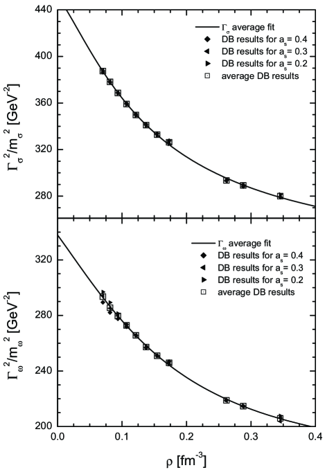
Figure 1: Effective density dependence of the $\sigma$ (upper part) and the $\omega$ (lower part) meson-nucleon vertices. Shown are results extracted from DB selfenergies from the Groningen NN potential [18] calculated for the asymmetry ratios $a_{s}=0.2,0.3,0.4$. The solid line is the asymmetry independent fit through the average of the DB results (open squares).

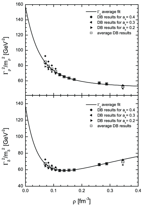
Figure 2: Same as Fig. 1 but for the $\rho$ (upper part) and $\delta$ (lower part) meson-nucleon vertices.

Several parameterizations of density dependent coupling constants exist. But they either only include density dependence in the isoscalar channel [20] due to the lack of asymmetric nuclear matter DB calculations or they are purely phenomenological [29]. Here we present a parameterization of asymmetric nuclear matter results [18, 31] derived from the Groningen potential [14, 32]. The mapping of the DB self-energies is done as proposed in equations (35) - (38) leading to a density dependence in both the isoscalar ($\sigma$, $\omega$) and the isovector ($\delta$, $\rho$) channel. Figure 1 and Fig. 2 show the dependence of the ratios $\frac{\Gamma_{\alpha}}{m_{\alpha}}(k_{F})$ on the density $\rho(k_{F})$ for different asymmetry ratios $a_{s}=\rho_{p}/\rho$. In the isoscalar channel the dependence on the asymmetry is negligible, in the iscovector channel it is extremely weak, especially around the saturation density of about $\rho_{0}=0.16fm^{-3}$. We therefore choose the ansatz that the coupling constant only depend on the total vector density $\rho(k_{F})$ and not on the proton and neutron densities separately. In order to take into account a maximum of information from the DB calculations we fit the average of the self-energies for the asymmetry ratios $a_{s}=0.2,0.3,0.4$ [18]. In [20] a polynomial expansion of $\Gamma^{2}$ in $k_{F}$ around the saturation density $k_{F_{0}}$ was chosen, leading to an excellent fit of the self-energies around $\rho_{0}$. But due to the polynomial approach the behavior at very low and very high densities is not perfectly stable. Intending applications over wide density regions ranging from nuclear halos to neutron star conditions in future investigations we choose a rational approximation as proposed in Ref. [29]

$$\Gamma_{\alpha}(\rho)=a_{\alpha}\left[\frac{1+b_{\alpha}(\frac{\rho}{\rho_{0}}+d_{\alpha})^{2}}{1+c_{\alpha}(\frac{\rho}{\rho_{0}}+e_{\alpha})^{2}}\right].$$ (45)

A clear advantage of such a rational form is the well defined behavior at low and high densities turning into a constant at very high densities. The results for the fit for $\rho_{0}=0.16fm^{-3}$ are displayed in Fig. 1 for the isoscalar channel and in Fig. 2 for the isovector channel of the interaction. The parameters are shown in Table 1. The description of the DB results is very good, in the isoscalar channel it is even sufficient to require $d_{\alpha}=e_{\alpha}$. In the isovector channel the fit is more difficult, especially since the $\delta$-meson has an ascending slope at high densities. This requires the additional parameter $e_{\alpha}$ to describe the low and the high density behavior equally well.

III.4 Results for infinite nuclear matter

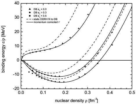
Figure 3: Equation of state for different asymmetry ratios $a_{s}$ calculated from the Groningen NN potential. DB results from [18] are represented by symbols. The dashed line shows the DDRH EoS for meson-nucleon vertices fitted to the DB self- energies, the solid line denotes results with momentum correction.

To check the quality of the effective parameterization (Table 1) of the in-medium dependence of the vertices it is instructive to look at the infinite nuclear matter EoS. The calculation was done by solving the meson field equations (13-16) with the densities from equations (28) and (29). Results for symmetric nuclear matter ($a_{s}=0.5$), pure neutron matter ($a_{s}=0.0$) and for nuclear matter with an asymmetry ratio of $a_{s}=0.3$ are shown in Fig. 3. Displayed are also the DB binding energies from [18] for the same NN potential. One sees that the equation of state is clearly not reproduced even though the fit describes the self-energies at $k_{F}$ very well. While the DB EoS has a binding energy of $\epsilon/\rho_{0}=-15.6$ MeV and a saturation density $\rho_{0}=0.182$ fm^-3, the standard choice leads to a Hartree EoS which is about 2.5 MeV weaker bound ($\epsilon/\rho_{0}=-13.13$ MeV) and the saturation density is shifted to lower densities ($\rho_{0}=0.161$ fm^-3). As discussed in Sec. III.2 due to the approximations made when neglecting the momentum dependence of the self-energies this could be expected.

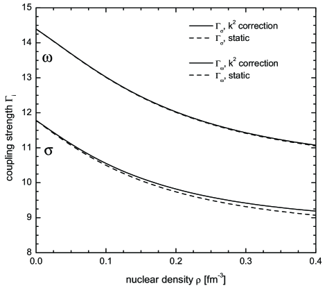
Figure 4: Momentum corrected density dependence of the $\sigma$ and $\omega$ meson-nucleon vertices. Results are shown for $\zeta_{\sigma}=0.00804$ fm^-2 and $\zeta_{\omega}=0.00103$ fm^-2 (solid line) and compared to the fits from Fig. 1 (dashed line).

We apply our momentum correction scheme to the coupling constants in a two step process. First we restrict ourselves to symmetric nuclear matter and try to reproduce the DB EoS by adjusting $\Gamma_{\sigma}$ and $\Gamma_{\omega}$. This is done in the constant momentum correction scheme by choosing $\zeta_{\sigma}$ and $\zeta_{\omega}$ in such a way that the saturation point of DB calculations is reproduced. We find the very small corrections $\zeta_{\sigma}=0.00804$ fm^-2 and $\zeta_{\omega}=0.00103$ fm^-2 and are able to reproduce the EoS very accurately as can be seen in Fig. 3. It is important to note that even though we only adjusted one point we are able to reproduce the binding energies at low as well as at high densities. This justifies our assumption of a $k_{F}^{2}$ dependence for the correction of the coupling constants. Figure 4 compares the momentum corrected couplings to the original ones. The correction increases with higher densities (or momenta) as expected from the functional form of the coupling constants but remains small for the $\sigma$ meson and nearly negligible for the $\omega$ meson. Nevertheless these small corrections suffice to gain 2.5 MeV binding energy at saturation density. We conclude that the EoS reacts extremely sensitive to small changes in the coupling constants, therefore great care has to be taken when fitting the self-energies. In addition the same is appropriate for DB calculations. One has to be very careful when extracting the self-energies and needs a consistent scheme for the projection onto the Lorentz invariants.

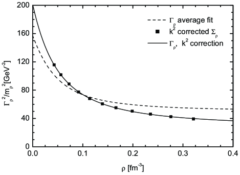
Figure 5: Momentum corrected density dependence of the $\rho$ meson- nucleon vertex. Results are shown for the fit (solid line) through the corrected self-energies and compared to the fit from Fig. 2 (dashed line).

After fixing $\Gamma_{\sigma}$ and $\Gamma_{\omega}$ the second step is to adjust the couplings in the isovector channel. This is done by keeping $\Gamma_{\delta}$ fixed and adjusting $\zeta_{\rho}$ for each given DB binding energy to neutron matter. In this approach one obtains a density dependent correction $\zeta_{\rho}(k_{F})$. The correction is incorporated in the DB self-energies and the $\rho$ meson-nucleon vertex is readjusted. The corrected self-energies and the fit through them are shown in Fig. 5, the parameters are given in Table 2. From Fig. 3 it is seen that the new fit reproduces the EoS of neutron matter very well and this even at high densities where the static fit to the DBHF self-energies leads to an interaction being far too repulsive. This is important for applications to neutron stars where the high density behavior plays a crucial role. Figure 3 also shows an excellent accordance of the calculations with DB results at intermediate asymmetry ratios, e.g. $a_{s}=0.3$, especially around the saturation density. This is a very important result since the interaction was only adjusted to pure neutron matter and justifies our assumption that the parameterization of meson-nucleon vertices is asymmetry independent. We also confirmed this for other values of $a_{s}$ where DB results were available from [18].

In Table 3 nuclear matter properties for the presented models are given. Saturation density and binding energy of the momentum corrected DDRH calculation reproduce the DB data very well, also the asymmetry-energy coefficient $a_{4}=26.1$ MeV, determined by

$$a_{4}=\rho_{0}^{2}\frac{\partial}{\partial(\rho_{3})^{2}}\frac{\epsilon}{\rho}(\rho_{0},\rho_{3})|_{\rho_{3}=0},$$ (46)

is in compliance with DB value of 25 MeV even though this value was not taken into account for the adjustment of the isovector interaction.

IV Relativistic Hartree Description of finite nuclei

IV.1 Properties of finite nuclei

The density dependent interaction derived in the preceding section for nuclear matter is now applied to finite nuclei in Hartree calculations. We solve the full meson field equations (13-17) and the Dirac equation (22) in coordinate space. The Dirac equation is solved for the upper and lower components of the eigenspinor $\psi_{b}$ simultaneously. The set of coupled equations is solved self-consistently under the assumption of spherical symmetry. Pairing effects in the particle-particle (p-p) channel have to be taken into account in open shell nuclei. Since we are mainly interested in the mean-field particle-hole (p-h) channel and especially in the isovector properties of the interaction, the BCS approximation was used. This is a standard procedure in relativistic and non-relativistic mean-field approaches. Following [37] a constant pairing matrix element of $G=2.15\text{ MeV}/\sqrt{A}$ was assumed and the standard set of BCS equations [38] was solved independently for protons and neutrons, respectively. In exotic nuclei close to the dripline pairing effects can be very important if the Fermi energy is close to the continuum. Here, relativistic Hartree-Bogoliubov (RHB) calculations, taking into account the coupling of bound states to the continuum, have been performed for phenomenological interactions [39, 40, 41] leading to excellent agreement with experimental results. We found in our calculations that pairing gives only minor to negligible contributions compared to the effects from the microscopic interaction in the p-h channel (less than 2% to the total binding energy of the Ni and Sn isotopes).

The center-of-mass correction which gives a significant contribution to the binding energy of light nuclei is treated in the usual harmonic oscillator approximation

$$E_{cm}=-\frac{3}{4}\hbar\omega\quad\text{with}\quad\hbar\omega=41A^{-1/3}\text{MeV}.$$ (47)

Then, the total ground state energy that has to be compared with experimental data is given by

$$E_{g.s.}=E_{\text{MF}}+E_{pair}+E_{cm}$$ (48)

where the Hartree ground state energy is obtained from the energy momentum tensor through spatial integration of its $T^{00}$ component.

$$E_{\text{MF}} = \sum_{i,\epsilon_{i}\leq\epsilon_{F}}v_{i}^{2}\epsilon_{i}-\int d^{3}r\rho(r)\Sigma^{0(r)}(r)$$ (49)

$$-\sum_{b=p,n}\frac{1}{2}\int d^{3}r\left[\rho_{b}^{s}(r)\Sigma_{b}^{s(0)}(r)-\rho_{b}(r)\Sigma_{b}^{0(0)}(r)\right]$$

$$+\frac{1}{2}\int d^{3}r\rho_{p}(r)eA^{(\gamma)}_{0}(r).$$

The $\epsilon_{i}$ are the Dirac eigenvalues of particles in positive energy eigenstates and energies less or equal the Fermi energy $\epsilon_{F}$ and the $v_{i}^{2}$ are the occupation probabilities obtained from BSC pairing.

In order to examine the effects of the density dependent isovector coupling constants, it is instructive to look at the mean-field potentials. In leading non- relativistic order the effective central potential $U_{b}^{C}$ is given by the difference of the strongly attractive scalar and repulsive vector fields

$$U_{b}^{C}=\Sigma_{b}^{0}-\Sigma_{b}^{s}$$ (50)

while the strength of the spin-orbit potential

$$U_{b}^{SO}=\frac{1}{2M}\frac{-\partial_{r}\left(\Sigma_{b}^{s}+\Sigma_{b}^{0}\right)}{E+M-\left(\Sigma_{b}^{s}+\Sigma_{b}^{0}\right)}$$ (51)

is determined by the sum of these fields.

Interestingly, the spin-orbit potential differs for protons and neutrons since the self-energies depend on the isospin. We define the isoscalar and isovector spin-orbit potentials as

$$U_{0}^{SO} = \frac{1}{2}\left(U_{n}^{SO}+U_{p}^{SO}\right)$$ (52)

$$U_{\tau}^{SO} = \frac{1}{2}\left(U_{n}^{SO}-U_{p}^{SO}\right)$$ (53)

as a measure for isovector spin-orbit interactions. We expect to see an enhancement of the isovector potential $U_{\tau}^{SO}$ due to the inclusion of the $\delta$ meson. While, to a large extend, the contributions of the $\rho$ and the $\delta$ mesons compensate each other in the central potential $U_{b}^{C}$, producing an effective isovector potential that is comparable in strength to the one obtained in calculations that include only the $\rho$ meson, the isovector self-energies of the $\rho$ and $\delta$ mesons add up and increase the isovector spin-orbit potential $U_{\tau}^{SO}$. This will be discussed in detail in the next section.

IV.2 Closed shell nuclei

As a first test of the momentum corrected density dependent interaction we examine closed shell nuclei. Nuclei considered in our calculations were the doubly magic nuclei ¹⁶O, ⁴⁰Ca, ¹⁰⁰Sn, ¹³²Sn, ²⁰⁸Pb, having major shell gaps at 8, 20, 50 and 82 for both protons and neutrons, as well as nuclei where one or both types of nucleons have only a minor (semimagic) shell gap at 28 or 40 (⁴⁸Ca, ⁴⁸Ni, ⁵⁶Ni, ⁶⁸Ni, ⁹⁰Zr). The nuclei have measured binding energies with very small errors [42] except for the proton rich nuclei. The binding energy of ¹⁰⁰Sn has been measured with a relatively large error [43]. ⁴⁸Ni, whose binding energy can be extrapolated in terms of the mirror binding energy difference to ⁴⁸Ca [37], has recently been produced experimentally [44]. The set of nuclei includes stable as well as $\beta$ unstable nuclei covering the range from the proton dripline to very neutron rich isotopes and allows us to investigate the interaction, determined from asymmetric nuclear matter, extensively on finite nuclei.

IV.2.1 Binding energies and charge radii

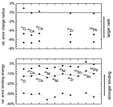
Figure 6: Relative errors for charge radii $(\rho_{c}-\rho_{c}^{\text{exp}})/\rho_{c}^{\text{exp}}$ (upper part) and binding energies $(E_{B}-E_{B}^{\text{exp}})/E_{B}^{\text{exp}}$ (lower part) obtained with the Groningen parameterization. Shown are results for magic and semimagic nuclei. Results without momentum correction are denoted by upper triangles, results for $\zeta_{\sigma}=0.00804$ fm^-2 and $\zeta_{\omega}=0.00103$ fm^-2 (adjusted to nuclear matter) by squares and results for $\zeta_{\sigma}=0.008$ fm^-2 and $\zeta_{\omega}=-0.002$ fm^-2 (adjusted to finitite nuclei) by circles. The lines are drawn to guide the eye.

In Table 5 we display results for closed shell nuclei calculated with the DDRH parameterization of the Groningen NN potential derived in Sec. III. Figure 6 shows the relative error for charge radii and binding energies compared to experimental results. The parameterization derived directly from the self-energies without momentum correction completely fails to describe the experimental results. While the charge radii are described very well, all nuclei are strongly underbound by about 30%. The proton dripline of the tin isotopes is already reached before ¹⁰⁰Sn due to the weak binding of the protons. But this had to be expected from the infinite nuclear matter results where the binding energy at saturation is also too weak. Applying the momentum correction from Sec. III.4, the results are greatly improved. While the binding energies are still underestimated by about 10%, compared to the static parameterization the improvement is remarkable. On the other hand, the size of the charge radii decreases, but with an error of about 4% the general agreement with experimental data is still satisfying.

Comparing our results with density dependent calculations for the Bonn A interaction [23, 25, 27], especially the description of the binding energies is less satisfactory, but the reason for this lies in the different NN potentials. While the parameterization of the Bonn A NN potentials has at a nuclear matter saturation density of $\rho_{0}=0.162$ fm^-3 an energy of about $-16.3$ Mev and for this reason tends to overbind finite nuclei, the saturation point of the Groningen NN potential is shifted to higher densities and the saturation energy is only about $-15.6$ MeV. These properties are clearly translated to finite nuclei, leading for the Groningen interaction to an underestimation of the binding energy, and a high nucleon density and deep mean-field potential inside the nuclei. The high saturation density stronger localizes the protons inside the nuclei leading to smaller charge radii. We compared the theoretical charge density to experimental results and found an overestimation of about 5% to 10% for all considered nuclei. Therefore, to improve results for finite nuclei, Brueckner calculations and NN potentials have to be improved first.

We were also interested in seeing how sensitive results for finite nuclei are to the momentum correction and if it is possible to improve results by adjusting the momentum correction factors $\zeta_{\alpha}$ to finite nuclei. No attempt was made to optimize the parameters in order to obtain a perfect fit of data. Isovector coupling constants remained unchanged. We found that a correction of $\zeta_{\sigma}=0.008$ fm^-2 and $\zeta_{\omega}=-0.002$ fm^-2 provides a reasonable description of both charge radii and binding energies. This modification essentially corresponds to a weakening of the repulsion of the vector self-energy compared to the original nuclear matter parameterization, but other modifications lead to similar results. It should be noted that our discussion of the momentum correction in infinite nuclear matter only partly applies to the $\zeta_{\alpha}$ determined for finite nuclei and that the strict relation to the factor $\Sigma^{\prime}/\Sigma^{\text{DB}}$ is not retained. Obviously, we implicitly take into account higher order effects and especially correct for the deficiencies of the NN potential in reproducing the binding energies of finite nuclei. This is demonstrated by the reversed sign of $\zeta_{\omega}$ compared to the nuclear matter value.

Results are shown in Table 5. As can be seen from Fig. 6, charge radii are further decreased while the agreement with the experimental binding energies is satisfying. In general, an improvement in the binding energies leads to smaller values for the charge radii and it is not possible to reproduce both observables simultaneously with the same Groningen parameter set. An improvement of the results would be possible by adjusting the $\sigma$ mass to better reproduce the charge radii but a phenomenological fit to experimental results was not the goal of our investigations.

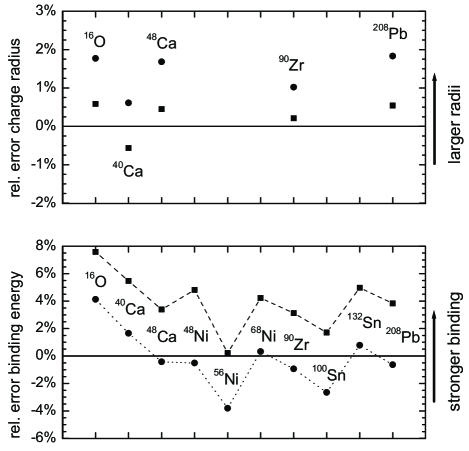
Figure 7: Same as Fig. 6 but for the Bonn A parameterization from [20, 23]. Results without momentum correction are denoted by squares and results for $\zeta_{\sigma}=-0.003$ fm^-2 and $\zeta_{\omega}=-0.0015$ fm^-2 by circles. The lines are drawn to guide the eye.

We also investigated if the momentum correction could possibly improve the description of finite nuclei for the Bonn nucleon potential. We used the parameterization of the Bonn A $\sigma$ and $\omega$ meson-nucleon vertices from [20] that was also applied to a few closed shell nuclei in [23, 25]. The $\rho$ coupling strength is chosen as $g_{\rho}^{2}/4\pi=5.19$ with a mass of $m_{\rho}=770$ MeV. Adjusting the momentum correction factors to the values $\zeta_{\sigma}=-0.0030$ fm^-2 and $\zeta_{\omega}=-0.0015$ fm^-2 leads to a good agreement with the experimental binding energies (except for some $N=Z$ nuclei where p-n pairing might be important) while preserving the good results for the charge radii. Results are presented in Table 6 and Fig. 7. One realizes the same behavior as for the Groningen parameterization. Now, a decrease in the binding energies leads to an overestimation of the charge radii.

The modification of the density dependent vertices is very small. Comparing the original fit of Haddad and Weigel [20] to the momentum corrected vertices we found that, in the density range important for finite nuclei, the reproduction of the nuclear matter self-energies is of the same accuracy. This leads to the conclusion that the momentum correction is clearly able to improve results and confirms our statement from Sec. III that bulk properties are very sensitive to small changes in the vertices.

We also recalculated the equation of state for the Bonn A potential with the modified vertices. Comparing to the original parameterization we found the agreement with the DB binding energy at saturation density to be slightly improved but not perfect. At low densities both parameterizations fail to reproduce the EoS. This seems to be a problem of the calculations of Brockmann and Machleidt who assumed a priori momentum-independent self-energies and fitted them only to the positive-energy matrix elements of the scattering matrix. We tried to adjust the coupling constants with our momentum correction procedure but were unable to resolve the inconsistency between the DB self-energies and the DB binding energy, e.g. to reproduce the EoS for all densities. This is not surprising considering the method of the DB calculations and the fact that the momentum correction is not able to change the global properties of the density dependence of the self-energies.

As can be seen from Figs. 6 and 7 the momentum correction always leads to a shift of the relative errors that is nearly identical across all considered nuclei. The reason is that the general properties of the interaction were not altered, these are already determined by the density dependence of the meson-nucleon vertices. Also the isovector part of the interaction remained unchanged. We conclude that the momentum correction is able to improve the extraction of the self-energies from Brueckner calculations preserving the microscopic structure of the NN interaction.

IV.2.2 Spin-orbit splitting

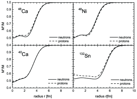
Figure 8: Isospin dependence of the effective masses of closed-shell nuclei from relativistic density dependent Hartree calculations using the parameterization of the Groningen NN potential.

As stated before, we expect the effects of including the $\delta$ meson to manifest in the isovector spin-orbit potential and in isovector dependent effective masses. In Fig. 8 effective masses for a representative sample of nuclei are displayed. While in the $N=Z$ nucleus ⁴⁰Ca the difference between proton and neutron masses is induced solely by Coulomb effects and is negligible, in the neutron rich nucleus ¹³²Sn the proton and neutron effective masses differ by about 10% at central density. This enhancement is caused by the isovector contribution to the scalar self- energy. The mirror nuclei ⁴⁸Ca and ⁴⁸Ni nicely demonstrate the effect of the scalar isovector density by showing a reversed behavior in the effective masses. We found that the momentum correction does not strongly effect the effective masses, only slightly decreasing (increasing) them due to a deeper (flatter) core potential.

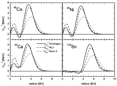
Figure 9: Spin-orbit potentials of closed-shell nuclei from DDRH calculations. Shown are the isoscalar potentials $U_{0}^{SO}$ for the Groningen parameterization (solid lines) and the Bonn A parameterization (dotted line). For comparison results calculated with the phenomenological NL3 RMF parameter set are shown (dashed lines).

The effective masses calculated with the Groningen potential are quite small, leading, together with the relatively large self-energies, to a large spin-orbit potential as can be seen from Fig. 9. Analogous to the effective masses no strong dependence on the momentum correction was found. For comparison we also display the spin-orbit potential of the Bonn A and the phenomenological NL3 parameter set [8]. The Bonn A spin-orbit potential is too small with the peak structure at the nuclear surface shifted to larger radii. We found the same behavior for the effective mass, being larger and less localized in the center of the nucleus. The properties of the Groningen and NL3 spin-orbit potentials are relatively similar, but the spin-orbit splitting of the Groningen potential is too large (about a factor two larger than the one obtained with Bonn A) as can be seen from Table 7. Compared to the NL3 parameterization that describes the experimental values well, $\Delta_{LS}$ is about 25% too strong, while for Bonn A it is about 30% too weak.

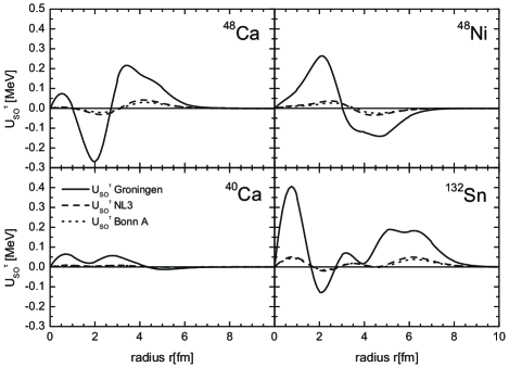
Figure 10: Same as Fig. 9 but for the isovector spin- orbit potentials $U_{\tau}^{SO}$.

Figure 10 illustrates the isovector dependence of the spin-orbit potential discussed in Sec. IV.1. While $U_{\tau}^{SO}$ has a non-negligible strength in neutron-rich nuclei and the mirror nuclei ⁴⁸Ca and ⁴⁸Ni its main contribution is not located at the nuclear surface. One could expect to see an effect comparing the spin-orbit splitting of neutrons and protons or mirror nuclei but we found no systematic behavior. The isovector spin-orbit potential does not seem to manifest itself strongly in the single particle energies and is probably overshadowed by the bulk isovector potential.

IV.3 Ni and Sn isotopes

The isotopic chains of Ni and Sn are of particular interest for nuclear structure calculations because of their proton shell closures at Z=28 (Z=50). They also extend from the proton dripline that is found nearby the doubly magic ⁴⁸Ni and ¹⁰⁰Sn nuclei to the already $\beta$ unstable neutron-rich doubly magic ⁷⁸Ni and ¹³²Sn isotopes. This allows us to investigate the isovector properties of the derived density dependent interactions and to test the interactions in regions far off stability. An extensive investigation of these nuclei can be found in [39, 48, 49] and the references therein.

IV.3.1 Binding energies

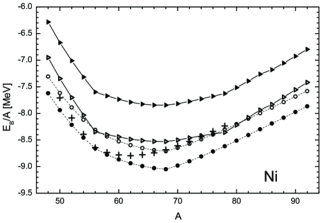
Figure 11: Binding energies per nucleon for the nickel isotopes. Shown are results with (open circles) and without momentum correction (solid circles) for the parameterizations of the Bonn A potential. Results derived from the Groningen parameter set are denoted by solid triangles (momentum corrections adjusted to nuclear matter EoS) and open triangles (adjusted to finite nuclei). Experimental binding energies are denoted by crosses (taken from Ref. [42]). The lines are drawn to guide the eye.

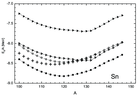
Figure 12: Same as Fig. 11 but showing binding energies of the tin isotopes.

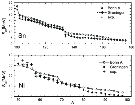
Figure 13: Two neutron separation energies for the nickel (lower part) and the tin (upper part) isotopes. Results for the Groningen (triangles) and Bonn A (circles) parameterization are shown. Experimental separation energies are denoted by crosses (taken from Ref. [42]). The lines are drawn to guide the eye.

Theoretical and experimental binding energies per nucleon are compared in Fig. 11 for nickel and in Fig. 12 for tin. The Groningen interaction derived from nuclear matter strongly underbinds the Ni and Sn isotopes. The reason for this was already discussed in Sec. IV.2. The adjusted parameter set describes neutron rich nuclei reasonably well but fails on the neutron-poor side. Agreement for the Sn isotopes is relatively poor. This is mainly caused by the extremely strong shell closure at N=82 that shifts the minimum of the binding energy from the experimental value of approximately ¹¹⁵Sn to the doubly magic ¹³²Sn. The reason is the too strong spin-orbit splitting of the Groningen potential that affects the subshell structure of the Sn isotopes and enhances the shell gap. Nevertheless, the correct shell structure is reproduced as can be seen from Fig. 13 where the two-neutron separation energies

$$S_{2n}(Z,N)=B(Z,N)-B(Z,N-2)$$ (54)

are compared with experimental values. The agreement is satisfying except for the too strong shell gaps for ¹³²Sn and ⁵⁶Ni. The momentum correction does not strongly affect $S_{2n}$ since it mainly shifts the binding energy of the isotopic chain not affecting the binding energy differences.

The Bonn A parameter set describes the neutron-poor Ni isotopes fairly well but overbinds the neutron-rich Ni and the Sn isotopes. On the other hand, agreement of the results for the momentum corrected interaction with experimental data on the neutron- rich side is very good but binding energies of neutron-poor isotopes are underestimated by 0.2 MeV. Also, comparing the two-neutron separation energies (Fig. 13), experimental results are reproduced well, but some deviations can be noticed. The shell gaps for ¹³²Sn and ⁵⁶Ni are relatively small whereas the gap for ⁶⁸Ni is too large. This also explains why the minimum of the binding energy is found at ⁶⁸Ni and the isotopes of the ⁵⁶Ni to ⁶⁸Ni shell are underbound. The reason for this probably lies in the weak spin-orbit splitting of the Bonn A potential.

Realizing that for N $\rightarrow$ Z nuclei only the Coulomb interaction determines the difference between the neutron and proton energies while the isovector interaction is strongly suppressed we conclude that the underbinding of the neutron- poor nuclei is caused by a too weak central isoscalar potential. On the other hand the neutron- rich isotopes are mostly affected by the isovector interaction that acts attractive for protons, balancing the Coulomb repulsion, and repulsive for neutrons. Since neutron-rich isotopes are described well this is an indication that for both the Groningen and the Bonn A potential the microscopic isovector potentials seem to be too weak. One can visualize this easily by shifting the curves in Figs. 11 or 12 vertically to reproduce the binding energy of $N=Z$ nuclei. This increases in first order only the isoscalar central potential. Then, the neutron-rich isotopes are overbound, indicating that the repulsion from the isovector potential is too weak.

IV.3.2 Density distributions

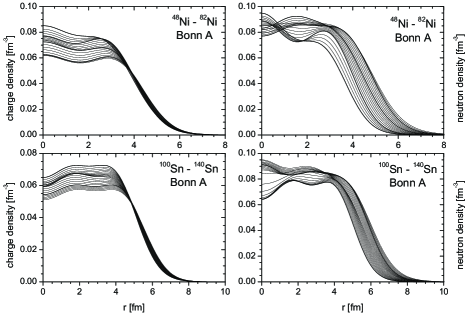
Figure 14: Charge and neutron density distributions for the isotopic chains of the Sn and Ni nuclei, calculated with the Bonn A parameter set.

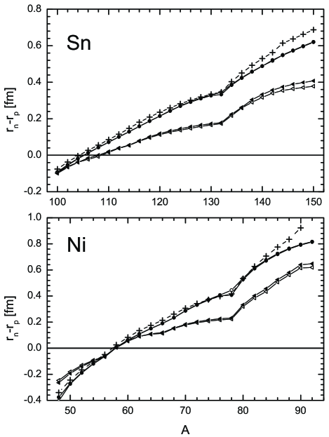
Figure 15: Difference of the root mean square radii of neutrons and protons of the nickel (lower part) and the tin (upper part) isotopes calculated with the Groningen (triangles) and Bonn A (circles) parameterizations. For comparison results calculated with the phenomenological NL3 RMF parameter set are shown (crosses). The lines are drawn to guide the eye.

Self-consistent neutron density distributions and charge densities for the Ni and Sn isotopes are displayed in Fig. 14. Closed shell nuclei are marked by bold lines. The distributions are only presented for the Bonn A potential but for the Groningen potential the same systematics is obtained. For the calculation of the charge density the theoretical point particle density distribution $\rho_{p}$ is folded with a Gaussian proton form factor [45] with $\sqrt{\langle r^{2}\rangle_{p}}=0.8$ fm. From ⁴⁸Ni to ⁷²Ni the charge density in the interior is reduced by about 30% accompanied by a mild increase of the charge radius by about 5%. For the neutron densities a more drastic evolution is found. Beyond ⁷⁸Ni (N=50 shell closure) the $2d_{5/2}$ subshell is being filled and a thick neutron skin is build up. This leads to sudden jump in the neutron rms radii while the proton rms radii increase only slowly. This behavior is more clearly visible in Fig. 15 where the differences of the proton and neutron rms radii are shown. Approaching the proton dripline a relative thick proton skin below N=28 is predicted. We also compare our results to calculations with the NL3 interaction. In Ref. [39] relativistic Hartree-Bogoliubov calculations for the Ni and Sn isotopes using this interaction were performed leading to excellent agreement with experimental data. Figure 15 shows very good agreement for the Bonn A potential with the results for the NL3 interaction. The Groningen potential has the same tendency but with smaller values. This is explained by the systematic underestimation of the rms radii (Fig. 6) that also causes a reduced difference between proton and neutron rms radii. Nevertheless, the same neutron skin is found. Since the Groningen potential leads to larger shell gaps for reasons of its strong spin-orbit potential, at the (sub)shell closure N=40 a small increase is already seen. Figure 15 also illustrates that the results are independent of the momentum correction. This is obvious since the correction only shifts all rms radii to higher or lower values.

The same calculations were performed for the Sn isotopes. In Fig. 14 density distributions from ¹⁰⁰Sn to ¹⁴⁰Sn are displayed showing the same neutron skin as the Ni isotopes. Here, one finds a sudden jump beyond N=82 where the $1h_{11/2}$ shell is filled and the $2f_{7/2}$ subshell becomes populated (Fig. 15). Again the agreement between the Bonn A and the NL3 parameter set is excellent. In Ref. [47] calculations for the Sn isotopes with non-relativistic interactions were performed and identical results were found. This shows that the observed neutron skins in Sn and Ni are relatively independent of the NN interaction and the theoretical approach.

V Summary and conclusion

We have extracted density dependent meson-nucleon vertices from DBHF self- energies of asymmetric nuclear matter, derived from realistic NN potentials. For the Groningen NN potential we found that the coupling constants can be expressed solely in terms of the nuclear matter baryon density $\rho$ and are independent of the asymmetry fraction for which the self-energies were calculated. The extraction of momentum- independent self-energies introduces errors in the density dependence of the interaction and leads to difficulties to reproduce the DB EoS in the DDRH approach. We introduced a momentum correction to account for this error and found excellent agreement of our calculated EoS for all asymmetry fractions $a_{s}=\rho_{p}/\rho$ with the Brueckner results. While the corrections are very small, the sensitivity of the saturation point of nuclear matter and the binding energies of finite nuclei to this correction is very high. This indicates the difficulty of extracting momentum independent coupling constants.

Applying the momentum corrected interaction to finite nuclei, we find that the agreement with experimental results is satisfactory, taking into account that the used parameterization contains no free parameters for finite nuclei. For the Groningen parameter set, the binding energy per nucleon is underestimated by 0.5 to 1 MeV whereas the charge radii are about 0.1 to 0.15 fm too small. These results are comparable with other mean-field calculations [25, 26, 27]. Using the Bonn A potential results are improved, indicating that the Groningen potential is not attractive enough, especially in the low density regime. We also adjusted the momentum correction factors to improve the description of the properties of finite nuclei. This leads to a good agreement with experimental data while keeping the excellent reproduction of the DB self- energies.

The inclusion of the $\delta$ meson introduces different effective masses for protons and neutrons and strongly enhances the isovector spin-orbit potential. However, we found no systematic effect in the isovector spin-orbit splitting. In order to further examine this effect, detailed experimental data for the single- particle energy levels and for exotic nuclei are necessary. Compared to phenomenological RMF interactions, we found the spin-orbit splitting of the Groningen potential to be enhanced and the one of the Bonn A potential to be suppressed. This becomes visible in the shell structure of some exotic nuclei. We also found indications that the isovector interaction of both microscopic interactions seems to be too weak to reproduce the complete isotopic chains of Sn and Ni correctly.

In general, we think that the results of the DDRH approach are quite satisfactory and that the momentum correction provides a consistent scheme to reproduce DBHF calculations and improve the agreement with finite nuclei. Improvements of the results could possibly be achieved by going beyond the ladder approximation and including, e.g., three-body interactions and ring diagrams. In future investigations we also plan to apply the density dependent interactions to neutron stars to gain additional insights in the properties of the isovector density dependence.

meson $\alpha$	$\sigma$	$\omega$	$\delta$	$\rho$
$m_{\alpha}$[MeV]	$550$	$783$	$983$	$770$
$a_{\alpha}$	$13.1334$	$15.1640$	$19.1023$	$12.8373$
$b_{\alpha}$	$0.4258$	$0.3474$	$1.3653$	$2.4822$
$c_{\alpha}$	$0.6578$	$0.5152$	$2.3054$	$5.8681$
$d_{\alpha}$	$0.7914$	$0.5989$	$0.0693$	$0.3671$
$e_{\alpha}$	$0.7914$	$0.5989$	$0.5388$	$0.3598$
$\rho_{0}=0.16$ [$fm^{-3}$]

Table 1: Parameterization of the density dependent couplings from equation (45) extracted from DB calculations in asymmetric nuclear matter[18].

$a_{\alpha}$	$b_{\alpha}$	$c_{\alpha}$	$d_{\alpha}$	$e_{\alpha}$
19.6270	1.7566	8.5541	0.7783	0.5746
$\rho_{0}=0.16$ [$fm^{-3}$]

Table 2: Parameterization of the $\rho$ meson-nucleon vertex after adjusting the neutron matter DDRH equation of state to the DB binding energy.

	DBHF	DDRH	DDRH corr.
$\rho_{sat}$ [$fm^{-3}$]	0.182	0.161	0.180
$\epsilon/\rho$ [MeV]	-15.5	-13.13	-15.60
$K$ [MeV]	–	211	282
$m^{*}/M$	–	0.592	0.554
$a_{4}$ [MeV]	25	28.2	26.1

Table 3: Comparison of infinite nuclear matter properties obtained in the DDRH model with results from DB calculations for the Groningen NN potential. Results are shown for calculations with and without momentum correction.

exp.	$r_{c}$[fm]	$E/A$[MeV/A]
16O	2.74	7.98
40Ca	3.48	8.55
48Ca	3.47	8.67
90Zr	4.27	8.71
208Pb	5.50	7.87
48Ni	–	7.27
56Ni	–	8.64
68Ni	–	8.68
100Sn	–	8.26
132Sn	–	8.26

Table 4: Experimental values of the rms charge radii and binding energies per nucleon for (semi)magic nuclei. Data are taken from Refs.[37, 42, 43, 46]

Groningen	$\zeta_{\sigma}=0.0$		$\zeta_{\sigma}=0.00804$ fm-2		$\zeta_{\sigma}=0.008$ fm-2
	$\zeta_{\omega}=0.0$		$\zeta_{\omega}=0.00103$ fm-2		$\zeta_{\omega}=-0.002$ fm-2
	$r_{c}$	$E/A$	$r_{c}$	$E/A$	$r_{c}$	$E/A$
16O	$2.76$	$5.65$	$2.61$	$7.00$	$2.56$	$7.56$
40Ca	$3.47$	$5.96$	$3.30$	$7.52$	$3.24$	$8.16$
48Ca	$3.48$	$6.09$	$3.31$	$7.79$	$3.25$	$8.49$
90Zr	$4.26$	$6.00$	$4.06$	$7.77$	$3.99$	$8.49$
208Pb	$5.49$	$5.28$	$5.24$	$7.10$	$5.15$	$7.84$
48Ni	$3.77$	$4.68$	$3.54$	$6.28$	$3.46$	$6.95$
56Ni	$3.73$	$5.78$	$3.53$	$7.60$	$3.46$	$8.35$
68Ni	$3.88$	$6.13$	$3.69$	$7.83$	$3.63$	$8.52$
100Sn	$(4.46)$	$(5.42)$	$4.24$	$7.25$	$4.16$	$8.00$
132Sn	$4.69$	$5.86$	$4.47$	$7.68$	$4.40$	$8.42$

Table 5: Root-mean-square charge radii $r_{c}$[fm] and binding energies per nucleon $E_{B}/A$ [MeV/A] of (semi)magic nuclei from density dependent relativistic Hartree (DDRH) calculations using the Groningen NN potential. Results for different momentum correction factors $\zeta_{\sigma}$ and $\zeta_{\omega}$ (see text) are shown. The values in parenthesis correspond to unbound nuclei.

Bonn A	$\zeta_{\sigma}=0.0$		$\zeta_{\sigma}=-0.0030$ fm-2
	$\zeta_{\omega}=0.0$		$\zeta_{\omega}=-0.0015$ fm-2
	$r_{c}$	$E/A$	$r_{c}$	$E/A$
16O	$2.75$	$8.58$	$2.79$	$8.30$
40Ca	$3.46$	$9.02$	$3.50$	$8.69$
48Ca	$3.49$	$8.96$	$3.53$	$8.63$
90Zr	$4.26$	$8.98$	$4.31$	$8.63$
208Pb	$5.53$	$8.17$	$5.60$	$7.82$
48Ni	$3.84$	$7.62$	$3.89$	$7.31$
56Ni	$3.79$	$8.66$	$3.84$	$8.31$
68Ni	$3.88$	$9.05$	$3.93$	$8.71$
100Sn	$4.51$	$8.40$	$4.57$	$8.04$
132Sn	$4.74$	$8.67$	$4.78$	$8.32$

Table 6: Same as Table 5 but with results for the Bonn A NN potential.

$\Delta_{LS}(n,p)$	16O	40Ca	48Ca	48Ni
Gron.	8.0/7.8	8.3/8.0	8.0/7.7	7.5/7.4
Gron. adj.	9.0/8.7	9.6/8.8	8.8/8.5	8.3/8.2
Bonn A	4.2/4.2	4.6/4.6	4.0/4.1	3.9/3.8
Bonn A adj.	4.0/4.0	4.4/4.3	3.7/3.8	3.6/3.6
exp.	6.1/6.3	6.3/7.2	5.6/4.3	–

Table 7: Neutron and proton spin-orbit splitting $\Delta_{LS}(n,p)$ in MeV for the $1p$ shell (¹⁶O) and the $1d$ (⁴⁰Ca, ⁴⁸Ca and ⁴⁸Ni) shell. Results are shown for the Groningen and the Bonn A NN potential, for the interaction derived from nuclear matter and for the adjustment to finite nuclei, respectively. For experimental values see Ref.[23]