HBT correlation functions from event generators - a reliable approach to determine the size of the emitting source in ultrarelativistic heavy ion collisions ?

Abstract

and R differ by up to $30\%$.

I Introduction

Which particle and energy densities are reached during an ultra relativistic heavy ion reaction? This is one of the present key questions in this field. If the density exceeds a critical value, theory predicts that a plasma, consisting of quarks and gluons, is produced whereas below that density the matter stays in its hadronic phase, consisting of mesons and baryons.

Theoretical predictions on the density and the energy density obtained in present (SPS) or future (RHIC and LHC) heavy ion reactions are rather vague because the understanding of the initial phase in which projectile and target become decelerated is still a theoretical challenge without a reliable answer yet. Therefore the present efforts concentrate on an experimental determination of these densities.

It is all but easy to measure coordinate space dependent quantities in heavy ion reactions. Single particle spectra contain direct information on the momentum space only. Therefore more complicated observables have to be employed to study the density. Probably the most powerful but certainly the most employed approach is based on a suggestion of Goldhaber, Goldhaber, Lee and Pais (GGLP) [1] who used the Hanbury-Brown and Twiss (HBT) effect [2]. It is based on the fact that the amplitudes of two indistinguishable processes interfere. If an object emits two identical bosons or fermions with momenta ${\bf k}_{1}$ and ${\bf k}_{2}$ which are registered by two detectors the dependence of the cross section ${d^{6}\sigma\over d^{3}k_{1}d^{3}k_{2}}$ on the relative distance between the detectors or on the relative momentum of the registered particles is an image of the emitting source. This method has been proven to be quite powerful for measuring the size of stars [2].

In heavy ion physics the situation is much more difficult:
a) There is nothing like a static source which emits particles. The system has a complicated geometrical structure and expands in space and time. Therefore not only one parameter (like in astrophysics the rms radius of a star) but the functional dependence of several parameters on time is encoded in the data.
b) There is no unique definition of when a particle is emitted because the emission is in reality a disconnection from the expanding system. Usually one assumes that after its last collision the particle can be considered as emitted. The space-time point of the last collision is called freeze out point.
c) There are long range Coulomb forces which change the particle momenta after emission.

Two approaches are possible in this situation:
A) One neglects the complications, limits the problems with the geometry by using only particles which are emitted at midrapidity and parameterizes the source with a couple of parameters. The parameters are then determined from the measured one and two particle cross sections [3]. For a review on the present status of this approach we refer to the recent paper of Wiedemann and Heinz [4]. The problem is that it is not easy to reveal the physical significance of the numerical values of these parameters.
B) One employs numerical simulation programs which have been validated by reproducing the measured single particle spectra. These programs, however, are semiclassical in their nature and hence particles and not wave functions are propagated. Therefore one has to extend these programs by a quantum calculation (classical particles do not interfere) if one would like to employ them for the prediction of the HBT correlation function. Here the rationale is as follows: If the extended program reproduces the correlation data, one can assume that it describes properly not only the momentum but also the coordinate space distribution of the particles. Hence the distribution of the particles in these simulation programs can be used to calculate densities and energy densities. The first suggestion to use the simulation programs to study the HBT effect has been advanced in [5]. Later Csörgö et al. [6] and Pratt et al. [7] have performed the first calculations using Fritjof, an event simulation program. In these calculations it has been assumed that a) the Coulomb interaction can simply be taken into account by multiplying the two particle Wigner density by the Gamow correction factor and b) one can identify the Wigner density of the nucleon with the classical phase space density. The latter is obtained by averaging the phase space points of the particles at the end of the simulation over many events. This has become the standard approach for a comparison of simulations and experiments [8]. Already in ref. [9] it has been found that in heavy ion collisions the Gamow correction factor overpredicts the true effects and rather a classical trajectory calculation has to be employed. Recently several propositions have been made to improve the treatment of the Coulomb interaction [10, 11, 12, 13]. The difference between the classical one body phase space density and the Wigner density of a emitted particle has been pointed out in [14].

Here we study these both assumptions. In particular, using one of the up to date simulation programs which reproduces the single particle spectra quite well (section 2), we study how the source parameters, obtained from the asymptotically observed correlation function, are related to the true source. This includes a study of the source (section 3), a study of the Wigner density of the emitted particles and its relation to the classical phase space density (section 4), a study of the influence of the Coulomb fields (chapter 5), a study of the influence of the resonance decay and a study of the kaon correlation function. We will show that the relation between the source and its image (coded in the correlation function) is all but simple and that the source density as determined by the correlation function may differ by a factor of two from that determined directly in the simulation program.

Whereas the study of the difference between the Wigner density and the classical phase space density and the consequences for the interpretation of the correlation function in terms of a source radius is rigorous, the study of the influence of the Coulomb interaction can be only considered as a first step. It shows the order of magnitude of the corrections one has to expect but present computer power does not allow to supplement the simulation programs by the solution of a Schrödinger equation to calculate the (anti)symmetrized wave function of the correlated pions in the field of all other charges.

II The method

A neXus

To study the space time structure of ultrarelativistic heavy ion collisions one has to rely on simulation programs like VENUS [15], neXus[16] or URQMD [17]. These event generators describe the reaction from the initial separation of projectile and target until the final state which is registered in the detectors. They assume that during the heavy ion reaction strings are formed which disintegrate into hadrons. The hadrons are treated semiclassically and can scatter among themselves elastically or inelastically before they are detected. For our study we use neXus (version 2.0 beta), the successor of VENUS, one of the most developed event generators, which describes the single particle spectra of the observed mesons and baryons at CERN energies quite well. We refrain from describing the details of this model and refer to ref. [16]. The program is used in its version without droplet formation in order to avoid the unknown Coulomb forces between droplets and hadrons. In using one of these models we follow here the common believe that up to the last strong interaction collision (freeze out) the hadrons are well described by a semiclassical approach.

B Implementation of the electromagnetic interaction in neXus

In order to study more rigorously the influence of the electromagnetic interaction on the two-particle correlation function we have to implement it directly into the simulation program. Because the average distance $r(t_{2})$ (where $t_{2}$ is the time when the later emitted hadron has its last collision) between the correlated hadrons is rather large (as we will see in part III) it is sufficient to implement the interaction on a semiclassical level [9, 18]. Correlated hadrons or pairs we call those pairs of particles which have a relative momentum smaller than 100 MeV. As we will see later the correlation function differs from one only for those pairs and hence only they carry information on the size of the system.

The electromagnetic interaction of a particle $i$ with another charged particle $j$ is given by

$$m_{i}\frac{du_{i}}{d\tau}=\sum_{j\neq i}\frac{e_{i}}{c}F_{ij}^{\mu\nu}u_{i}^{\nu}.$$ (1)

Here j runs over all charged particles of the system. The particle $i$ has the mass $m_{i}$, the charge $e_{i}$ and the 4-velocity $u_{i}=\{1,{\bf v}\}/\sqrt{1-{\bf v}^{2}}$. The tensor $F_{ij}^{\mu\nu}$ is given by

$$F_{ij}^{\mu\nu}=\frac{e_{j}}{c}\frac{X^{\mu}u_{j}^{\nu}-X^{\nu}u_{j}^{\mu}}{(\frac{1}{c^{2}}(u^{\lambda}_{j}X^{\lambda})^{2}-X_{\lambda}X^{\lambda})}$$ (2)

where $X^{\lambda}$ is the relative 4 - distance between the particles $i$ and $j$.

The formula  (1) assumes point like particles and the absence of acceleration of the particle j. In our case this is a valid assumption because at high energies the electromagnetic force changes the momenta only little. Applying this formalism at each time step in the neXus program (which updates the particle positions and momenta at common light cone times) we create Coulomb trajectories of all charged particles.

For the analysis presented later we store the mutual Coulomb force between all charged particles at all time steps. Whether two mesons form a correlated pair we know only at the end of the simulation. Using these stored forces we can separate the change of the relative momentum of the pair particles $\mbox{${\bf k}$}_{S}$ due to their mutual interaction ($\Delta\mbox{${\bf k}$}_{pair}$) from that due to their interaction with the environment (i.e. all other charged particles)($\Delta\mbox{${\bf k}$}_{environ}$). The final relative momentum of the correlated pair $\mbox{${\bf k}$}_{final}$ is

$$\mbox{${\bf k}$}_{S}+\Delta\mbox{${\bf k}$}_{environ}+\Delta\mbox{${\bf k}$}_{pair}=\mbox{${\bf k}$}_{final}.$$ (3)

As we will see in this classical trajectory calculation the average change of the relative momentum of the correlated pair particles due to their mutual Coulomb interaction is about as large as that due to the interaction with the environment. This suggests that also in a quantal calculation both are equally important. The importance of the Coulomb interaction between a particle and its environment can also be seen experimentally by comparing the measured $\pi^{+}$ and $\pi^{-}$ spectra as done in fig.1.

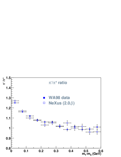
FIG. 1.: $\pi^{-}$ spectrum divided by the $\pi^{+}$ spectrum, both obtained by the WA98 collaboration [11], as compared to the NeXus result.

We see that at relative momenta smaller than 100 MeV the spectra differ considerably and that this difference is well reproduced by the neXus calculation including the classical Coulomb interaction. This relative momentum has to be compared with the relative momentum ${\bf k}$ for which the correlation function $C(\mbox{${\bf k}$})$ becomes one and hence ceases to carry information on the source size. As we will see later ${\bf k}$ is as well around 100 MeV. Hence the influence of the Coulomb interaction on the correlation function cannot be neglected.

III Space time structure of the source

The first question we address is when and where the particles, which are finally seen in the detectors, are created. We limit ourselves to pions emitted at midrapidity $y_{cm}-1\leq y\leq y_{cm}+1$. For our study we use the reaction Pb + Pb at 158 AGeV for b $\leq$ 3.2 fm. Fig.2 top presents the distribution of freeze out times of charged mesons. We display this time separately for particles created by string decay, by resonance decay or inelastic collisions, and by elastic collisions. We see no sudden freeze out, rather a distribution which is almost flat between 3 and 10 fm/c. Without rescattering we would have seen one peak at 1 fm/c (string breaking) and another one around 5 fm/c ($\rho$ decay ).

The distribution of transverse distances $R_{T}=\sqrt{x^{2}+y^{2}}$ of pions at freeze out with respect to the center of the reaction is displayed in the middle part of the figure. We observe as well a rather flat distribution followed by a very long tail which ranges up to 18 fm! Hence according to the simulation program rescattering made it impossible to define a unique radius of the system at freeze out which could hopefully be measured. The transverse momentum distribution of the pions does not strongly depend on their origin. This can be concluded from the bottom part of fig.2, where the momentum distribution of the pions is displayed.

FIG. 2.: Distribution of freeze out times, freeze out radii and freeze out momenta for charged $\pi$’s with $y_{cm}-1<y<y_{cm}+1$ from neXus+Coulomb. Black squares show particles from string fragmentation, open circles show pions from elastic collisions and open triangles those from resonance decay or from inelastic collisions.

More interesting than the average properties of all particles are that of those pions, which finally have a small relative momentum with respect to another pion of the same charge state. We will see later that the correlation function differs from 1 only for those pairs of particles which have a relative momentum smaller than 100 MeV. These pairs we call correlated pairs and only they carry information on the size of the system.

The distribution of freeze out times $t_{2}$ of those pairs can be directly translated into a distribution of source sizes $R_{source}(t_{2})=\sqrt{{1\over N_{pion}}\sum_{all\ pions}{\bf r}_{i}(t_{2})^{2}}$. This distribution of source sizes is displayed in fig.3 for two cases: for all pairs and for those pairs where none of the pions come from resonance decay. We see a broad distribution with a maximum at 8 (10)fm and a mean value of 11.3 (12.4)fm. For calculating the mean value we have omitted all particles beyond $R_{source}$ = 30 fm, i.e. pions which come from long living resonances like $\omega$ or $\Lambda$.

Thus there is neither a common freeze out time nor a common freeze out volume.

FIG. 3.: Distribution of source sizes for pairs with a relative momentum of less than 100 MeV.

FIG. 4.: Distribution of relative distances at freeze out for pairs with a final momentum of $k<100MeV$ in comparison with that of all pairs of positively charged pions.

In fig.4 we compare the distribution of the relative distance $r(t_{2})$ at freeze out for the correlated pairs in comparison with that for all pion pairs. First of all, the average distance is above 10 fm. We observe furthermore that the average value for the small relative momentum pairs ($\sqrt{<r^{2}(t_{2})>}$ = 10.8 fm) differs considerably from that for all pairs ($\sqrt{<r^{2}(t_{2})>}$ = 15.6 fm). Consequently, the pairs with a small relative momentum are not representative for all pairs. This one has to keep in mind if one likes to interpret the correlation function in terms of physical source radii.

FIG. 5.: Momentum-position correlation in the neXus model.

The difference between the distribution of relative distances of pairs with $k<100MeV$ and that of all pairs is a consequence of strong space - momentum space correlations, in beam (z) direction as well as in the direction of the impact parameter (x). These correlations of freeze out momenta and positions are displayed in fig. 5 and are well known. They give rise to the identity of rapidity and space time rapidity. We see that even in the small rapidity interval around midrapidity, in which we perform our investigation, these correlations are by far not negligible.

Now, after we have described the source, we can investigate to which extend its properties can be recovered by measuring correlation functions.

IV The correlation function without electromagnetic interactions

A The formalism

All semiclassical simulation programs propagate classical particles which have a sharp momentum ${\bf k}_{A}$and a sharp position ${\bf r}_{A}$. This is conceptually necessary in order to determine the sequence of collisions and the center of mass energy of each collision. On the other hand, two particles emitted with sharp momenta and sharp positions do not interfere because their trajectories are distinguishable. In order to model physics which is based on the interference of wave functions, like the HBT effect, one has to treat the particles as quantum particles for which the uncertainty principle is fulfilled. Therefore a transition from classical to quantal physics is necessary. In view of the construction of the simulation programs this transition can only be made after the last collision.

This transition from classical to quantal physics requires more than the knowledge of ${\bf k}_{A}$and ${\bf r}_{A}$ provided by the simulation programs. In order to construct a wave function one needs at least one additional parameter (the width of the wave function) which is not provided by the simulation program. A popular choice for the wave function is a Gaussian superposition of plane waves. This wave function requires only one unknown parameter, the variance L/4, and there is even hope that its physical relevance can be understood, as we will see.

Two identical particles emitted at $t_{1}$ and $t_{3}$ at the source points ${\bf r}_{A}$ and ${\bf r}_{B}$ with the momenta centered around ${\bf k}_{A}$ and ${\bf k}_{B}$ observed in detectors with the momenta ${\bf k}_{1}$ and ${\bf k}_{2}$ can have two indistinguable trajectories. Either the particle emitted at ${\bf r}_{A}$ arrives with momentum ${\bf k}_{1}$ (and that from ${\bf r}_{B}$ with momentum ${\bf k}_{2}$)

$$A_{1} = \int d\mbox{${\bf p}_{1}$}d\mbox{${\bf p}_{2}$}<\mbox{${\bf k}_{1}$},t_{2}|t_{1},\mbox{${\bf p}_{1}$}><\mbox{${\bf p}_{1}$},t_{1}|\Phi_{A}>$$ (5)

$$\cdot<\mbox{${\bf k}_{2}$},t_{4}|t_{3},\mbox{${\bf p}_{2}$}><\mbox{${\bf p}_{2}$},t_{3}|\Phi_{B}>$$

or that emitted at ${\bf r}_{A}$ arrives with momentum ${\bf k}_{2}$ and correspondingly that emitted at ${\bf r}_{B}$ with ${\bf k}_{1}$

$$A_{2} = \int d\mbox{${\bf p}_{1}$}d\mbox{${\bf p}_{2}$}<\mbox{${\bf k}_{1}$},t_{2}|t_{1},\mbox{${\bf p}_{1}$}><\mbox{${\bf p}_{1}$},t_{1}|\Phi_{B}>$$ (7)

$$\cdot<\mbox{${\bf k}_{2}$},t_{4}|t_{3},\mbox{${\bf p}_{2}$}><\mbox{${\bf p}_{2}$},t_{3}|\Phi_{A}>.$$

For the wave function of the emitted particle

$$<\mbox{${\bf p}_{1}$},t_{1}|\Phi_{A}>=f_{A}(\mbox{${\bf p}_{1}$})e^{i\mbox{${\bf p}_{1}$}\mbox{${\bf r}_{A}$}}e^{-i\mbox{${\bf p}_{1}$}^{2}t_{1}/2m}$$ (8)

we assume a Gaussian form

$$f_{A}(\mbox{${\bf p}_{1}$})=({L\over 2\pi})^{3/4}e^{-(\mbox{${\bf p}_{1}$}-\mbox{${\bf k}_{A}$})^{2}L/4}.$$ (9)

If L is large the momentum of the particle is close to the source momentum but we loose the information on the source position. If L is small we have the opposite scenario.

$<\mbox{${\bf k}_{1}$},t_{2}|t_{1},\mbox{${\bf p}_{1}$}>=\delta^{(3)}(\mbox{${\bf k}_{1}$}-\mbox{${\bf p}_{1}$})e^{-i\mbox{${\bf p}_{1}$}^{2}(t_{2}-t_{1})/2m}$ is the propagator in momentum space. Because both trajectories are indistinguishable their amplitudes have to be added to obtain the correlation function

$$C^{(2)}(\mbox{${\bf k}$})={\int d\mbox{${\bf K}$}|A_{1}+A_{2}|^{2}\over\int d\mbox{${\bf K}$}(A_{1}^{2}+A_{2}^{2})}$$ (10)

$$= {g(\mbox{${\bf k}$}-\mbox{${\bf k}_{S}$})+g(\mbox{${\bf k}$}+\mbox{${\bf k}_{S}$})+2g(\mbox{${\bf k}$})g(\mbox{${\bf k}_{S}$})cos(2\mbox{${\bf k}$}\mbox{${\bf r}_{S}$})\over g(\mbox{${\bf k}$}-\mbox{${\bf k}_{S}$})+g(\mbox{${\bf k}$}+\mbox{${\bf k}_{S}$})}$$ (11)

where $\mbox{${\bf k}$}={\mbox{${\bf k}_{1}$}-\mbox{${\bf k}_{2}$}\over 2}\ ,\mbox{${\bf K}$}=(\mbox{${\bf k}_{1}$}+\mbox{${\bf k}_{2}$})\ ,\mbox{${\bf k}_{S}$}={\mbox{${\bf k}_{A}$}-\mbox{${\bf k}_{B}$}\over 2}\ ,\mbox{${\bf r}_{S}$}=(\mbox{${\bf r}_{A}$}-\mbox{${\bf r}_{B}$})$ and $g(\mbox{${\bf k}$})=({L\over\pi})^{3/4}e^{-\mbox{${\bf k}$}^{2}L}$. In our calculation we update the coordinates of the first emitted particle until the emission of the second particle of the correlated pair (at $t_{2}$). Therefore $cos(k_{\mu}r^{\mu})=cos\mbox{${\bf k}$}\mbox{${\bf r}$}$ where $r_{\mu}=\{0,\mbox{${\bf r}$}(t_{2})\}$ and the time component of the 4-vector of the relative distance disappears from the correlation function. If the two bosons have the same source momentum (${\bf k}_{A}$=${\bf k}_{B}$) and are measured in the detector with the same momentum we obtain an enhancement of $C^{(2)}(\mbox{${\bf k}$})$ by a factor of two as compared to distinguishable particles. However, if the source momenta are different, the result is more complicated.

If L is sufficiently small, the difference in the arguments of the exponential functions can be neglected and we obtain

$$C^{(2)}_{SM}(\mbox{${\bf k}$})={g(\mbox{${\bf k}$}-\mbox{${\bf k}_{S}$})(1+e^{-\mbox{${\bf k}$}^{2}L}cos(2\mbox{${\bf k}$}\mbox{${\bf r}_{S}$}))\over g(\mbox{${\bf k}$}-\mbox{${\bf k}_{S}$})}.$$ (12)

This approximation is called smoothness assumption. It is frequently used in the literature for the following reason: The measured correlation function can be well described by a Gaussian function [14]

$$C({\mbox{${\bf k}$}})=1+\lambda exp(-{4R^{2}}\cdot\mbox{${\bf k}$}^{2})$$ (13)

where $\lambda$ allows for the correction of a possible coherence in the source or for pairs of non identical particles. Assuming that the emission points have as well a Gaussian distribution in coordinate and momentum space

$$S(\mbox{${\bf k}_{S}$},\mbox{${\bf r}_{S}$})\propto e^{-\mbox{${\bf k}_{S}$}^{2}B}e^{-\mbox{${\bf r}_{S}$}^{2}/C},$$ (14)

where ${\bf k}_{S}$ and ${\bf r}_{S}$ are the relative distances in momentum and coordinate space, the convolution of $C^{(2)}_{SM}(\mbox{${\bf k}$})$ with the source distribution function S(${\bf k}_{S}$,${\bf r}_{S}$) yields

$$C_{SM}(\mbox{${\bf k}$})=$$ (15)

$${\int d\mbox{${\bf r}_{S}$}d\mbox{${\bf k}_{S}$}S(\mbox{${\bf k}_{S}$},\mbox{${\bf r}_{S}$})g(\mbox{${\bf k}$}-\mbox{${\bf k}_{S}$})(1+e^{-\mbox{${\bf k}$}^{2}L}cos(2\mbox{${\bf k}$}\mbox{${\bf r}_{S}$})\over\int d\mbox{${\bf r}_{S}$}d\mbox{${\bf k}_{S}$}S(\mbox{${\bf k}_{S}$},\mbox{${\bf r}_{S}$})g(\mbox{${\bf k}$}-\mbox{${\bf k}_{S}$})}$$ (16)

$$=1+e^{-\mbox{${\bf k}$}^{2}(L+C)}.$$ (17)

(18)

The apparent source size ${4R^{2}}$ is, in the Gaussian source approximation, four times the sum of the variance of the source C/4 and of that of the wave function squared L/4. In this approximation we find the following relation between the root mean square radius of the freeze out points $\sqrt{<r(t_{2})^{2}>}$ and the apparent source radius

$$<r(t_{2})^{2}>=3R^{2}=3/4(L+C).$$ (19)

Thus in the smoothness approximation one has only to fit the experimentally observed correlation function by a function of the form of eq.13 and can then use eq. 19 to determine the desired $<r(t_{2})^{2}>$. Consequently one can avoid to perform a Fourier transform, a difficult task in view of the large experimental error bars. In addition this equation is easy to interpret.

In the simulation programs we do not have a continuous source distribution. Rather we have to sum over all emission points:

$$C(\mbox{${\bf k}$})={\sum\int d\mbox{${\bf K}$}|A_{1}^{i}+A_{2}^{i}|^{2}\over\sum\int d\mbox{${\bf K}$}(|A_{1}^{i}|^{2}+|A_{2}^{i}|^{2})}$$ (20)

which yields in the smoothness approximation

$$C_{SM}(\mbox{${\bf k}$})=$$ (21)

$${\sum_{s=1}^{N_{ev}}\sum_{i=1}^{N_{pairs}}(1+e^{-\mbox{${\bf k}$}^{2}L}cos(2\mbox{${\bf k}$}\mbox{${\bf r}_{S}$}_{s,i}))*g(\mbox{${\bf k}$}-\mbox{${\bf k}_{S}$}_{s,i})\over\sum_{s=1}^{N_{ev}}\sum_{i=1}^{N_{pairs}}g(\mbox{${\bf k}$}-\mbox{${\bf k}_{S}$}_{s,i})}.$$ (22)

$N_{pairs}$ is the number of pairs in the event s.

Now it is important to realize which information is needed to calculate a correlation function and which information is to our disposal in these simulation programs. As seen in eqs. 5,7,20,22 we need
a) the single particle wave function for the two correlated particles emitted from emission points with relative coordinates ${\bf r}_{S}$ and ${\bf k}_{S}$.
b) the distribution of emission points. Because in the derivation of the correlation function [14] the source is treated classically these emission points $\mbox{${\bf r}_{S}$},\mbox{${\bf k}_{S}$}$ are either given by a source function like eq.14 or as a sum of delta functions in coordinate and momentum space as in eq.20,22.
The simulation programs treat the rescattering of the hadrons like the scattering of classical billiard balls. Only initially, when the hadrons are created by string decay, quantum mechanical constraints are taken into account. Consequently, the simulation programs present the time evolution of a classical chaotic system whose initial configuration is inspired by quantum mechanics. Hence we have to our disposal the classical n-body phase space density. Assuming that emission takes place at freeze out the classical n-body phase space density allows to calculate the emission points.

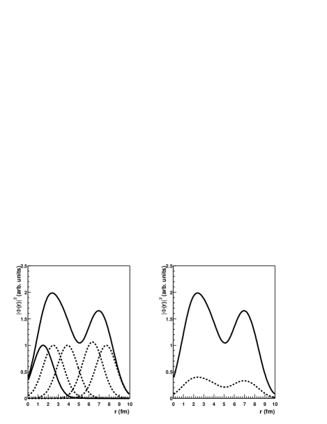
FIG. 6.: 2 different sets of single particle wave functions squared $\sum_{i}\mid\Phi_{i}(r)\mid^{2}$ which give the same one body Wigner density $\int F_{W}^{1}(r,k)dk$. On the right hand side $\mid\Phi_{i}(r)\mid^{2}=(\int F_{W}^{1}(r,k)dk)/5$.

It has been argued in the past [21, 20] that the knowledge of the classical n-body phase space density is sufficient to determine the single particle wave function as well. The argument goes as follows: From the classical n-body phase space density we can construct the classical one body phase space density (we use the nonrelativistic formulas here because there the argument becomes more transparent)

$$F^{1}_{cl}(\mbox{${\bf r}$},\mbox{${\bf k}$},t)=\sum_{i=1}^{n}\delta^{(3)}(\mbox{${\bf k}$}-\mbox{${\bf k}$}_{i}(t))\ \delta^{(3)}(\mbox{${\bf r}$}-\mbox{${\bf r}$}_{i}(t)).$$ (23)

Averaged over many events[21] or over one event [20] the classical one body density can be identified with the quantal one body Wigner density

$$F^{1}_{W}(\mbox{${\bf r}$},\mbox{${\bf k}$},t)={1\over N_{ev}}\sum_{N_{ev}}\sum_{i=1}^{n}g(\mbox{${\bf k}$},\mbox{${\bf r}$},\mbox{${\bf k}$}_{i}(t),\mbox{${\bf r}$}_{i}(t))$$ (24)

where $g(\mbox{${\bf k}$},\mbox{${\bf r}$},\mbox{${\bf k}$}_{i}(t),\mbox{${\bf r}$}_{i}(t))$ is the Wigner density of the single particle wave function $\Phi(\mbox{${\bf k}$},\mbox{${\bf k}$}_{i}(t),\mbox{${\bf r}$}_{i}(t))$ defined as

$$g(\mbox{${\bf k}$},\mbox{${\bf r}$},\mbox{${\bf k}$}_{i}(t),\mbox{${\bf r}$}_{i}(t)) = \int{d\mbox{${\bf q}$}\over(2\pi)^{3}}e^{i\mbox{${\bf q}$}\mbox{${\bf r}$}}\Phi^{*}(\mbox{${\bf k}$}+\mbox{${\bf q}$}/2,\mbox{${\bf k}$}_{i}(t),\mbox{${\bf r}$}_{i}(t))$$ (25)

$$\cdot \Phi(\mbox{${\bf k}$}-\mbox{${\bf q}$}/2,\mbox{${\bf k}$}_{i}(t),\mbox{${\bf r}$}_{i}(t)).$$ (26)

Now one assumes that all $\mbox{${\bf k}$}_{i}(t),\mbox{${\bf r}$}_{i}(t)$ are identical. Then we can identify

$$F^{1}_{W}(\mbox{${\bf r}$},\mbox{${\bf k}$},t)=n\cdot g(\mbox{${\bf k}$},\mbox{${\bf r}$})$$ (27)

Knowing $g(\mbox{${\bf k}$},\mbox{${\bf r}$})$ one can calculate the amplitudes $A_{1}$ (eq.5) and $A_{2}$ (eq.7).

There are, however, three shortcomings in this argument:
1) There is an infinity of single particle wave functions $\Phi$(eq.26) which give the same one body Wigner density (eq.24). They yield, however, quite different correlation functions. Fig.6 shows as example two sets of single particle wave functions which give the same one body Wigner density but different two body correlations C(k). Thus eq. 27 is one out of an infinity of choices of a single particle wave function for a given one body Wigner density. One may wonder if this is a good choice because it ignores all correlations between the $\mbox{${\bf k}$}_{i}(t)^{\prime}s$ and $\mbox{${\bf r}$}_{i}(t)^{\prime}s$. In addition it is difficult to motivate why until freeze out the particles are treated as point like in coordinate and momentum space whereas thereafter they are well described by a wave function for which $\Delta k\Delta r>>\hbar$. It is more natural to replace the precise momenta and positions of the particles by the ”most classical” wave functions around the classical $\mbox{${\bf k}$}_{i}(t)^{\prime}s$ and $\mbox{${\bf r}$}_{i}(t)^{\prime}s$, i.e. Gaussians which fulfill the uncertainty principle. In general, the ignorance of L and the impossibility to derive from the known one body Wigner density the single particle wave functions are two ways to express the same unknown physics.

Averaging over many events raises even more questions:
2) Two particles emitted next to each other (i.e. those which are finally interfering strongly) have a mutual Coulomb repulsion, which introduces a two body correlation between the pair even on the classical level. Averaging over many events (which means to allow that particles from different events interfere) destroys this correlation. Thus event averaging destroys correlations already present on the classical level.
3) There is no proof that the classical n-body phase space density averaged over many events is equivalent to the quantal one body Wigner density. On the contrary there are good reasons that this is not the case, if the size of the system is comparable to the width of the single particle wave function: If all particles are sitting on top of each other a classical n-body density is point like whereas the Wigner density has to obey the uncertainty principle.

For the determination of the correlation function from experimental data the denominator is obtained by event mixing. For our theoretical studies this is not necessary. Therefore we would not like to comment here on the consequences of the event mixing procedure for the correlation function. Numerically we observe quite a difference in the results if we replace the denominator of eqs.20,22 by the corresponding quantity for mixed events. This is caused by mutual Coulomb interactions (see 2)) which get lost by event mixing.

B The Correlation Function in neXus without electromagnetic interactions

As discussed, for a Gaussian source (eq.14) with no space-momentum space correlations there is a simple relation between the true source radius and the apparent source radius (eq.19).

Is this observation also true for the source as given by the simulation programs? This is the seminal question which we will discuss in this and in the next paragraphs. In the simulation programs we are confronted with three different source radii

• the classical source radius $R_{class}=\sqrt{<r(t_{2})^{2}}>$ as given by the simulation program where $<..>$ means averaging over all pions which are part of a pair. Their radius is taken at the time when the later emitted pair particle has its last collision. The distribution of $r(t_{2})^{2}$ ( i.e. of the freeze out points) is displayed in fig. 7. We see that this distribution deviates from a Gaussian form. It can be considered approximately as a sum of two Gaussians.

• the true source radius $R_{true}$ given by the rms radius of the system after the freeze out points have been convoluted with a Gaussian wave function squared of a variance of L/4. This source radius is called true because it is the relevant source radius if one wants to determine densities or energy densities and it is also the source radius the correlation function should ”measure”. For L=0 $R_{true}=R_{class}$.

• the apparent source radius R as given by eq.13. This apparent source radius can be calculated from the correlation function using the formalism derived in the last section. This is the only radius which can be measured experimentally.

FIG. 7.: Distribution of the freeze out points.

We start the investigation by calculating the correlation function (eq.20 or eq.22) of identically charged pions at midrapidity for different values of the variance L/4. We discard for the beginning those pairs which contain pions coming from resonance decay. These correlation functions have a form which can be well described by eq.13. We can therefore determine R by fitting the simulation results with a function of the form of eq.13. In fig.8 we display this dependence of the fit parameter $R^{2}$ on L. We separate the results obtained with (eq.22) and without (eq.20) the smoothness assumption.

Per definition for L=0 both agree. For larger values they differ by not more than 10% and hence the smoothness assumption is acceptable for the analysis of the results of the simulation programs. For the unrealistic case that $\sqrt{L}$ is large as compared to the source we see the expected (see eq.19) linear behavior, but this is not true anymore if $\sqrt{L}<R_{class}$, for the smoothness assumption as well as for the exact calculation.

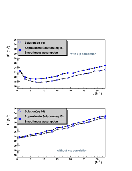
FIG. 8.: The square of the apparent source radius $R^{2}$ as a function of the variance L/4 of the single particle wave function squared. We display calculations with and without smoothness assumption. In the bottom figure we have artificially decorrelated the positions and momenta of the particles. $R^{2}$ is obtained by fitting the correlation function with $C(\mbox{${\bf k}$})=1+\lambda exp(-4\mbox{${\bf k}$}^{2}R^{2})$.

In order to understand the origin of this deviation from the expected behavior we decorrelate position and momentum of the pions. We attribute to each pion with a given source momentum a position randomly chosen among the source positions of the other pions. The result is displayed in the bottom panel of fig.8. We see now the expected behavior: The apparent source size increases if the width of the wavefunction and hence the true source radius increases.

In fig. 9 we plot the true source radius as a function of the apparent source radius. As explained, both can be obtained independently in the simulation program. Without space-momentum space correlations the apparent source radius follows the true source size, the convolution of the classical source with the single particle wave function squared, which can be independently calculated in the simulation program. The absolute values are, however, different. The reason for this difference is that the distribution of emission points (fig. 7) is not a Gaussian (despite of the fact that the correlation function can be well described by a Gaussian).

If we include the correlations generated in the simulation program the apparent source radius is, however, a quite complicated function the true source radius. Assuming that the apparent source size is the true source size one overpredicts the density of the source by up to a factor of 2. Thus we conclude that for the reaction investigated here the true source radius cannot even approximately be inferred from the apparent radius without a detailed knowledge of the space-momentum space correlations . We just like to mention that the experiments yield apparent source sizes which are considered as too small in order to be the true source size, a fact which, according to our results, may have its explanation in space-momentum space correlations.

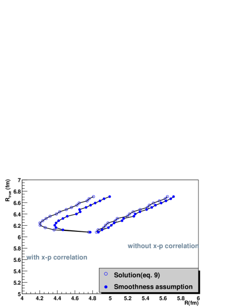
FIG. 9.: The true source size $R_{true}$ (as given by the simulation program) as a function of the apparent source size R determined by fitting the calculated correlation function by $C(\mbox{${\bf k}$})=1+\lambda exp(-4\mbox{${\bf k}$}^{2}R^{2})$ including (see fig. 8 top) and excluding (see fig. 8 bottom) space-momentum space correlations.

We would like to add two remarks:
a) The space-momentum space correlation in the simulation program is not created by flow. It is already caused by the string dynamics and is modified later due to rescattering. Thus adding only a radial (or in plane) flow to models which have otherwise no correlations between space and momentum space would not reduce the difference between R and $R_{true}$.
b) Being forced to introduce L as a free parameter we have lost the predictive power of the simulation programs as far as two body correlations are concerned. Instead of predicting the two body correlation function we can only state whether there is a value of L for which the simulation program reproduces the measured apparent source radius R. (As said the different values of $R_{true}$ are obtained by folding the same classical source distribution with the square of wave functions with different variances L/4.)

V Simulations including electromagnetic interactions

A The momentum change due to the electromagnetic interaction

After freeze out and during their way to the detectors the mesons change their momentum due to the Coulomb interaction. In fig. 10

FIG. 10.: Distribution of the change of the relative momentum between the particles of a correlated pair after freeze out. We separate the change due to the electromagnetic interaction with the environment (black circle), with the other pion of the correlated pair (open cross), and the sum of both (open circle).

we display the distribution of the change of the relative momentum of the correlated pairs between $t_{2}$ and detection, separated into the different origins. The average momentum change is of the order of 25 MeV and the interaction between the correlated pair contributes as much as the interaction of the pair particles with the environment. Even if these numbers are based on classical trajectory calculations, presented in section II, it is evident that calculations which take into account only one of these effects are not suited for the situation at hand.

B Standard treatment of electromagnetic interactions

As said already, the correlation function $C(\mbox{${\bf k}$})$ differs from one only for pairs with a relative momentum $k=\sqrt{(\mbox{${\bf k}_{1}$}-\mbox{${\bf k}_{2}$})^{2}}<100MeV$. Only these pairs carry information on the size of the system. The change of the relative momentum of a correlated pair due to the Coulomb interaction is of the same order of magnitude and therefore not negligible.

This is well known since long and several attempts have been made to correct the two body correlation function for the electromagnetic interaction [10, 11, 12, 13]. The correlation function $C(\mbox{${\bf k}$},\mbox{${\bf K}$})$ for a pair of particles emitted with a center of mass momentum ${\bf K}$ and an asymptotic relative momentum ${\bf k}$ is given by the square of the projection of the particle wave function $\phi^{K}({\bf r})$ , where ${\bf r}$ is the relative distance of the pair particles, onto the Coulomb wave function $\Phi^{coul}_{k/2}(\mbox{${\bf r}$})$,

$$C(\mbox{${\bf k}$},\mbox{${\bf K}$})=\int d^{3}r|<\Phi^{coul}_{k/2}|\mbox{${\bf r}$}><\mbox{${\bf r}$}|\phi^{K}>|^{2}.$$ (28)

$\Phi^{coul}_{k/2}(\mbox{${\bf r}$})$ is the solution of

$$({-\nabla^{2}_{{\bf r}}\over 2\mu}+V(\mbox{${\bf r}$}))\Phi^{coul}_{k/2}(\mbox{${\bf r}$})={\mbox{${\bf k}$}^{2}\over 2\mu}\Phi^{coul}_{k/2}(\mbox{${\bf r}$}).$$ (29)

Assuming identical freeze out points for the two particles $|\phi^{K}(\mbox{${\bf r}$})|^{2}=\delta^{3}(\mbox{${\bf r}$})$ we obtain the so called Gamow correction factor

$$G(\eta)=|\Phi_{k/2}^{coul}(r=0)|^{2}=\frac{2\pi\eta}{exp[2\pi\eta]-1}$$ (30)

with $\eta=\mu\alpha/k$ , $\mu$ the reduced mass. Often the ”Coulomb corrected” correlation function at freeze out is calculated by dividing the measured correlation function by the Gamow correction factor.

This approach has been recently critically studied and extended to a system of n bosons by Alt et al. [13]. They have shown that in a certain limit the n-body wave function can be approximated by the product of the relative wave functions of all pairs and that for small source sizes ($\approx 1fm$) this product can be replaced by that of the relative wave functions at zero relative distance. Then the Coulomb correction is nothing else than a product of Gamow correction factors. However, already for sources of 5 fm this product of correction factors overestimates the true Coulomb correction [13]. In view of the large source size we see in neXus (fig.3) these results elucidate why the Gamow correction does not work well for heavy ion reactions at ultrarelativistic energies, as has been observed in [22, 23, 24, 25].

C The correlation function in presence of electromagnetic fields

The above mentioned quantal approaches for the Coulomb correction are implicitly based on the assumption that the correlated pair particles are emitted very close to each other. Only then the environment changes the momentum of the pair particles by the same amount, leaving the relative momentum k unchanged. In this case one can solve eq.29. This is not the situation we see in the simulations. There the change of the relative momentum of a correlated pair particles due to the mutual Coulomb interaction is of the same order of magnitude as that due to the interaction with all the other particles. Then eq. 29 is not anymore a good approximation even more it is not even calculable: the asymptotic relative momenta k, necessary to calculate the Coulomb wave functions, are only known at the very end of the simulation, after the mutual Coulomb interactions have ceased, and are based in our approach on classical trajectory calculations. Thus we are left with the fact, that if quantal effects are important, our asymptotic relative momenta, based on a classical calculation are not correct, on the contrary, if they are correct quantal effects are negligible and we can live with calculating Coulomb corrections classically, as done here. Thus the quantal Coulomb correction proposed in [13] are incompatible with semiclassical simulation programs.

It has been proposed as well to replace in the Coulomb wave function the asymptotic momentum by the momentum at freeze out. For many applications this is certainly a very good approximation, but in our context it is not useful: this ansatz would eliminate the effect we would like to study: How the correlation function is modified by the interaction of the pair particles with the environment.

We would like to mention another problem which renders the application of a static quantal Coulomb correction in the context of semiclassical simulation programs quite difficult: Coulomb interactions and strong interactions cannot be separated in time. The earlier emitted pair particle has moved already in a (strong) Coulomb field when the later emitted one has its last collision.

Due to these problems even the most modest quantal approach, to describe the correlated pair by a two body wave function in which all other charges are treated in the Born Oppenheimer approximation, i.e. by supplementing in the Hamiltonian of eq. 29 $V(\mbox{${\bf r}$})$ by the Coulomb interaction with all other charged particles $\sum_{k}(V^{C}(\mbox{${\bf r}$}_{ik},t)+V^{C}(\mbox{${\bf r}$}_{jk},t)$, and then to solve the time dependent version of this equation, is not feasible with present day computers.

What can we do in this situation? Because the exact calculation is not possible we employ approximative methods to study the influence of the electromagnetic interaction on the correlation function. These approximations are crude, too crude probably to yield quantitatively reliable results, but sufficiently precise to demonstrate that more precise methods have to be developed before a quantitative relation between the apparent radius and the true source radius of the system can be established.

Our approximation consist in assuming that the momentum transfer due to the electromagnetic interaction is instantaneous. Under this assumption we study two cases. First we assume that the change of the momentum due to the electromagnetic interaction happens immediately at freeze out. This result is then compared with calculations which assume that the instantaneous momentum change happens at t, the time where in neXus on the average half of the momentum change has happened. t is of the order of 20 fm/c. Because the momentum change due to the electromagnetic interaction is moderate it does not completely destroy the correlation function obtained by neglecting the electromagnetic interaction (as for example collisions with large momentum transfer would do). Rather one expects a smooth modification.

The first case is easy to study. We have only to replace ${\bf k}_{S}$ by ${\bf k}_{S}$+${\bf q}$ where ${\bf q}$$=\Delta\mbox{${\bf k}$}_{pair}+\Delta\mbox{${\bf k}$}_{environment}$ is the momentum change due to the electromagnetic interaction. The second case requires a more careful study. As said, in order to create a correlation function one has to describe the mesons after freeze out by a wave function with a finite width in coordinate and momentum space. Therefore, if we take the quantum character of the mesons seriously, we have now 4 different amplitudes which are visualized in fig.9.

$$B_{1} = \int d\mbox{${\bf p}_{1}$}d\mbox{${\bf p}_{2}$}d\mbox{${\bf p}_{3}$}d\mbox{${\bf p}_{4}$}d\mbox{${\bf p}_{5}$}d\mbox{${\bf p}_{6}$}$$

$$<\mbox{${\bf k}_{1}$},t_{2}|t_{1},\mbox{${\bf p}_{5}$}>\delta(\mbox{${\bf p}_{3}$}+\mbox{${\bf q}_{1}$}-\mbox{${\bf p}_{5}$})<\mbox{${\bf p}_{3}$},t_{1}|0,\mbox{${\bf p}_{1}$}>$$

$$<\mbox{${\bf p}_{1}$},0|\Phi_{A}><\mbox{${\bf k}_{2}$},t_{2}|t_{1},\mbox{${\bf p}_{6}$}>\delta(\mbox{${\bf p}_{4}$}+\mbox{${\bf q}_{2}$}-\mbox{${\bf p}_{6}$})$$

$$<\mbox{${\bf p}_{4}$},t_{1}|0,\mbox{${\bf p}_{2}$}><\mbox{${\bf p}_{2}$},0|\Phi_{B}>$$

$$= <\mbox{${\bf k}_{1}$}-\mbox{${\bf q}_{1}$},t_{1}|\Phi_{A}><\mbox{${\bf k}_{2}$}-\mbox{${\bf q}_{2}$},t_{1}|\Phi_{B}>$$

$$B_{2} = \int d\mbox{${\bf p}_{1}$}d\mbox{${\bf p}_{2}$}d\mbox{${\bf p}_{3}$}d\mbox{${\bf p}_{4}$}d\mbox{${\bf p}_{5}$}d\mbox{${\bf p}_{6}$}$$

$$<\mbox{${\bf k}_{1}$},t_{2}|t_{1},\mbox{${\bf p}_{6}$}>\delta(\mbox{${\bf p}_{4}$}+\mbox{${\bf q}_{2}$}-\mbox{${\bf p}_{6}$})<\mbox{${\bf p}_{4}$},t_{1}|0,\mbox{${\bf p}_{1}$}>$$

$$<\mbox{${\bf p}_{1}$},0|\Phi_{A}><\mbox{${\bf k}_{2}$},t_{2}|t_{1},\mbox{${\bf p}_{5}$}>\delta(\mbox{${\bf p}_{3}$}+\mbox{${\bf q}_{1}$}-\mbox{${\bf p}_{5}$})$$

$$<\mbox{${\bf p}_{3}$},t_{1}|0,\mbox{${\bf p}_{2}$}><\mbox{${\bf p}_{2}$},0|\Phi_{B}>$$

$$= <\mbox{${\bf k}_{1}$}-\mbox{${\bf q}_{2}$},t_{1}|\Phi_{A}><\mbox{${\bf k}_{2}$}-\mbox{${\bf q}_{1}$},t_{1}|\Phi_{B}>$$

$$B_{3} = \int d\mbox{${\bf p}_{1}$}d\mbox{${\bf p}_{2}$}d\mbox{${\bf p}_{3}$}d\mbox{${\bf p}_{4}$}d\mbox{${\bf p}_{5}$}d\mbox{${\bf p}_{6}$}$$

$$<\mbox{${\bf k}_{1}$},t_{2}|t_{1},\mbox{${\bf p}_{6}$}>\delta(\mbox{${\bf p}_{4}$}+\mbox{${\bf q}_{2}$}-\mbox{${\bf p}_{6}$})<\mbox{${\bf p}_{4}$},t_{1}|0,\mbox{${\bf p}_{2}$}>$$

$$<\mbox{${\bf p}_{2}$},0|\Phi_{B}><\mbox{${\bf k}_{2}$},t_{2}|t_{1},\mbox{${\bf p}_{5}$}>\delta(\mbox{${\bf p}_{3}$}+\mbox{${\bf q}_{1}$}-\mbox{${\bf p}_{5}$})$$

$$<\mbox{${\bf p}_{3}$},t_{1}|0,\mbox{${\bf p}_{1}$}><\mbox{${\bf p}_{1}$},0|\Phi_{A}>$$

$$= <\mbox{${\bf k}_{1}$}-\mbox{${\bf q}_{2}$},t_{1}|\Phi_{B}><\mbox{${\bf k}_{2}$}-\mbox{${\bf q}_{1}$},t_{1}|\Phi_{A}>$$

$$B_{4} = \int d\mbox{${\bf p}_{1}$}d\mbox{${\bf p}_{2}$}d\mbox{${\bf p}_{3}$}d\mbox{${\bf p}_{4}$}d\mbox{${\bf p}_{5}$}d\mbox{${\bf p}_{6}$}$$

$$<\mbox{${\bf k}_{1}$},t_{2}|t_{1},\mbox{${\bf p}_{5}$}>\delta(\mbox{${\bf p}_{3}$}+\mbox{${\bf q}_{1}$}-\mbox{${\bf p}_{5}$})<\mbox{${\bf p}_{3}$},t_{1}|0,\mbox{${\bf p}_{2}$}>$$

$$<\mbox{${\bf p}_{2}$},0|\Phi_{B}><\mbox{${\bf k}_{2}$},t_{2}|t_{1},\mbox{${\bf p}_{6}$}>\delta(\mbox{${\bf p}_{4}$}+\mbox{${\bf q}_{2}$}-\mbox{${\bf p}_{6}$})$$

$$<\mbox{${\bf p}_{4}$},t_{1}|0,\mbox{${\bf p}_{1}$}><\mbox{${\bf p}_{1}$},0|\Phi_{A}>$$

$$= <\mbox{${\bf k}_{1}$}-\mbox{${\bf q}_{1}$},t_{1}|\Phi_{B}><\mbox{${\bf k}_{2}$}-\mbox{${\bf q}_{2}$},t_{1}|\Phi_{A}>.$$

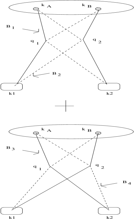
FIG. 11.: The 4 indistinguishable different amplitudes if the electromagnetic interaction happens instantaneously, with a momentum transfer of ${\bf q}_{2}$ and ${\bf q}_{1}$ .

Calculating $|\sum_{l}B_{l}|^{2}$ we find after integration over the center of mass motion:

$$Re(B_{1}B_{2}^{*})=D\cos(2\mbox{${\bf q}$}(\mbox{${\bf r}_{S}$}+2\mbox{${\bf k}$}\mbox{${t/m}$}))e^{-(\mbox{${\bf k}$}-\mbox{${\bf k}_{S}$})^{2}L-\mbox{${\bf q}$}^{2}L}$$

$$Re(B_{1}B_{3}^{*})=D\cos(2\mbox{${\bf k}$}(\mbox{${\bf r}_{S}$}+2\mbox{${\bf q}$}\mbox{${t/m}$}))e^{-(\mbox{${\bf q}$}+\mbox{${\bf k}_{S}$})^{2}L-\mbox{${\bf k}$}^{2}L}$$

$$Re(B_{1}B_{4}^{*})=D\cos(2\mbox{${\bf r}_{S}$}(\mbox{${\bf k}$}-\mbox{${\bf q}$}))e^{-(\mbox{${\bf k}$}-\mbox{${\bf q}$})^{2}L-\mbox{${\bf k}_{S}$}^{2}L}$$

$$Re(B_{2}B_{3}^{*})=D\cos(2\mbox{${\bf r}_{S}$}(\mbox{${\bf k}$}+\mbox{${\bf q}$})))e^{-(\mbox{${\bf k}$}+\mbox{${\bf q}$})^{2}L-\mbox{${\bf k}_{S}$}^{2}L}$$

$$Re(B_{2}B_{4}^{*})=D\cos(2\mbox{${\bf k}$}(\mbox{${\bf r}_{S}$}-2\mbox{${\bf q}$}\mbox{${t/m}$}))e^{-(\mbox{${\bf q}$}-\mbox{${\bf k}_{S}$})^{2}L-\mbox{${\bf k}$}^{2}L}$$

$$Re(B_{3}B_{4}^{*})=D\cos(2\mbox{${\bf q}$}(\mbox{${\bf r}_{S}$}-2\mbox{${\bf k}$}\mbox{${t/m}$}))e^{-(\mbox{${\bf k}$}+\mbox{${\bf k}_{S}$})^{2}L-\mbox{${\bf q}$}^{2}L}$$

$$B_{1}B_{1}^{*}=De^{-(\mbox{${\bf k}$}-\mbox{${\bf q}$}-\mbox{${\bf k}_{S}$})^{2}L}$$

$$B_{2}B_{2}^{*}=De^{-(\mbox{${\bf k}$}+\mbox{${\bf q}$}-\mbox{${\bf k}_{S}$})^{2}L}$$

$$B_{3}B_{3}^{*}=De^{-(\mbox{${\bf k}$}-\mbox{${\bf q}$}+\mbox{${\bf k}_{S}$})^{2}L}$$

$$B_{4}B_{4}^{*}=De^{-(\mbox{${\bf k}$}+\mbox{${\bf q}$}+\mbox{${\bf k}_{S}$})^{2}L}$$

where D contains the normalization. The exact result $C(\mbox{${\bf k}$})={|\sum B_{l}|^{2}\over\sum|B_{l}|^{2}}$ is too complex to discuss the physics. Therefore we apply the smoothness assumption, i.e we assume that all exponential functions can be approximated by $e^{-(\mbox{${\bf k}$}-\mbox{${\bf q}$}-\mbox{${\bf k}_{S}$})^{2}L}$. Then we obtain

$$C_{SA}(\mbox{${\bf k}$}) = (\sum_{s=1}^{N_{ev}}\sum_{i=1}^{N_{pairs(s)}}e^{-(\mbox{${\bf k}$}-\mbox{${\bf q}$}-\mbox{${\bf k}_{S}$}_{s,i})^{2}L}$$ (36)

$$(1+0.5\times e^{-(\mbox{${\bf k}$}-\mbox{${\bf q}$})^{2}L}\;cos(2\mbox{${\bf r}_{S}$}_{s,i}(\mbox{${\bf k}$}-\mbox{${\bf q}$}))+$$

$$0.5\times e^{-(\mbox{${\bf k}$}+\mbox{${\bf q}$})^{2}L}\;cos(2\mbox{${\bf r}_{S}$}_{s,i}(\mbox{${\bf k}$}+\mbox{${\bf q}$}))+$$

$$e^{-\mbox{${\bf k}$}^{2}L}\;cos(2\mbox{${\bf r}_{S}$}_{s,i}\mbox{${\bf k}$})cos(4\mbox{${\bf q}$}\mbox{${\bf k}$}\mbox{${t/m}$})+$$

$$e^{-\mbox{${\bf q}$}^{2}L}\;cos(2\mbox{${\bf r}_{S}$}_{s,i}\mbox{${\bf q}$})cos(4\mbox{${\bf q}$}\mbox{${\bf k}$}\mbox{${t/m}$}))$$

$$/(\sum_{s=1}^{N_{ev}}\sum_{i=1}^{N_{pairs(s)}}e^{-(\mbox{${\bf k}$}-\mbox{${\bf q}$}-\mbox{${\bf k}_{S}$}_{s,i})^{2}L}).$$

If ${\bf k}$ is equal 0 the correlation function is not anymore two but $\propto 1+e^{-\mbox{${\bf q}$}^{2}}\;cos(2\mbox{${\bf r}$}\mbox{${\bf q}$})$. For finite ${\bf k}$ and if ${\bf q}$ is small we find $C_{SA}(\mbox{${\bf k}$})=2(1+e^{-\mbox{${\bf k}$}^{2}L}cos(2\mbox{${\bf k}$}\mbox{${\bf r}_{S}$}))$ and hence up to a normalization constant the same result as in section IV. It is important to realize that the change of the momentum due to the electromagnetic forces modifies the result in a nonlinear way.

This general result will be compared later with that obtained under the assumption that ${\bf q}_{1}$ is the momentum transfer of the particle emitted with the momentum ${\bf k}_{A}$ (and correspondingly that the particle emitted with ${\bf k}_{B}$ suffers a momentum transfer of ${\bf q}_{2}$).

D The correlation function in neXus including electromagnetic interactions

Before discussing our results in detail we compare the calculated correlation function for $\pi^{+}\pi^{+}$ and $\pi^{-}\pi^{-}$ correlations in fig.12. Here we have assumed that the change of the momentum due to the electromagnetic interaction happens at $t_{2}$ and we choose $L=0fm^{2}$.

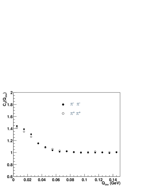
FIG. 12.: Correlation functions for $\pi^{+}\pi^{+}$ and $\pi^{-}\pi^{-}$ pairs emitted at midrapidity in 158 GeV/N Pb+Pb central collisions

As observed experimentally (fig. 1) the correlation function is almost identical for $\pi^{+}$ and $\pi^{-}$ pairs even including the Coulomb interaction in distinction to the single particle spectra (fig. 1). Please note that (as discussed in section IV A) the correlation function would be strongly modified if one uses mixed events for the normalization. In true simulation events the correlated pair particles suffer from a mutual Coulomb interaction before freeze out, whereas in mixed events this not the case.

We present now our results for three different scenarios. All are based on the assumption that the momentum transfer due to the Coulomb potential is instantaneous. In the first scenario we assume that the change of the momentum due to the electromagnetic interaction happens at $t_{2}$, in the second and third scenario that it happens at the time when in the classical trajectory calculation on the average half of the momentum change due to the electromagnetic interaction has occurred. The latter scenario is calculated for two different assumptions. First we assume that the particle emitted at A suffers a momentum change of ${\bf q_{1}}$ (and that emitted at B changed its momentum by ${\bf q_{2}}$). Then only the trajectories $B_{1}$ and $B_{3}$ of fig.11 are allowed. Finally we admit all 4 amplitudes $B_{1}-B_{4}$.

Fig.13 displays the correlation function under the assumption that the momentum transfer happens immediately at freeze out. We separate 4 different source momenta to discriminate the different origins of momentum change: a)${\bf k}_{S}$ momentum at freeze out (No Coulomb) b)${\bf k}_{S}$ + ${\bf\Delta k_{environ}}$ (Environment), the change of the relative momentum of the pair due to the interaction with the environment. c)${\bf k}_{S}$ + ${\bf\Delta k_{pair}}$ (Pairs), the change of the relative momentum of the pair particles due to their mutual Coulomb interaction and d)${\bf k_{final}}$=${\bf k}_{S}$ + ${\bf\Delta k_{pair}}$ + ${\bf\Delta k_{environ}}$ (All). The correlation functions are rather similar and the fit yields very similar results for R. Due to the fact that we don’t mix events for the determination of the denominator of eq.20, this result was expected. Event mixing would create a shift of the maximum to a finite value of $Q_{int}$ due to the lack of Coulomb repulsion between the particles from different events.

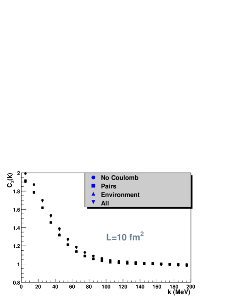
FIG. 13.: Correlation functions for 4 different final momenta (see text). We assume that the momentum transfer due to electromagnetic interaction happens at freeze out. L is assumed to be = $10fm^{2}$.

If we assume that the momentum transfer happens at 10 fm/c resp. 20 fm/c after $t_{2}$ and admitting only the amplitudes $B_{1}$ and $B_{3}$ we observe the dependence of the true source on the apparent source radius R as displayed in fig.14. For a given source size $R_{true}$ the Coulomb interaction increases the measurable apparent source size. The later the momentum transfer happens the larger is this change. For a given $R_{true}$ a momentum transfer at 20 fm/c may increase of the apparent source size radius by as much as 25%. No Coulomb is identical with the curve displayed in fig.9. We like to mention that the change of the apparent source radius due to the Coulomb interaction is of the order of magnitude expected from the schematic study in ref. [9].

If we allow for all 4 different amplitudes $B_{1}-B_{4}$ we see another time a quite different behavior. The correlation function has not anymore a Gaussian form as can be seen in fig.15. Fitting only the low momentum component by a Gaussian function one obtains R values which are slightly lower than if only the amplitudes $B_{1}$ and $B_{3}$ are allowed. The error bars of the fit are, however, large. We would like to mention that the non Gaussian form of the correlation function becomes only evident in our approach. If the correlation function is normalized by event mixing an overall normalization appears. Because the correlation function is normalized to 1 at large values of k this overall normalization absorbs the large ${\bf k}$  offset seen in fig.15.

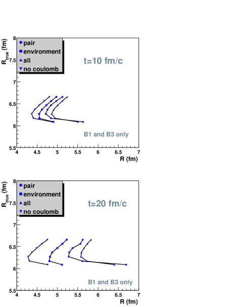
FIG. 14.: The true source radius $R_{true}$ (as given by the simulation program) as a function of the apparent source radius R determined by $C({\bf k})=1+\lambda exp(-{4\bf k}^{2}R^{2})$ including the Coulomb interaction (see text). We admit here only the amplitudes $B_{1}$ and $B_{3}$ (see text) and assume that the momentum transfer due to the electromagnetic interaction takes place at t= 10 fm/c (left) or at 20 fm/c (right).

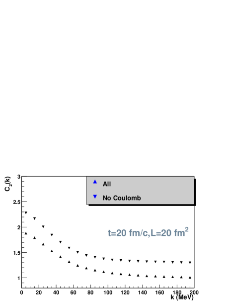
FIG. 15.: Correlation function obtained for the general case where all amplitudes $B_{1}-B_{4}$ (see text) are admitted. We assume that the momentum transfer takes place at t= 20 fm/c. The correlation function is not anymore Gaussian.

The influence of the pions from resonance decay on the correlation function is rather weak although the resonances can decay very late, when the distance to its pair partner is very large. This large distance increases $R_{true}$ tremendously. Therefore we have excluded them up to now from the analysis. The apparent source radius of all pairs as compared to pairs of particle where no pion comes from resonance decay is displayed in fig.16 as a function of L (L/4 being the variance of the wave function).

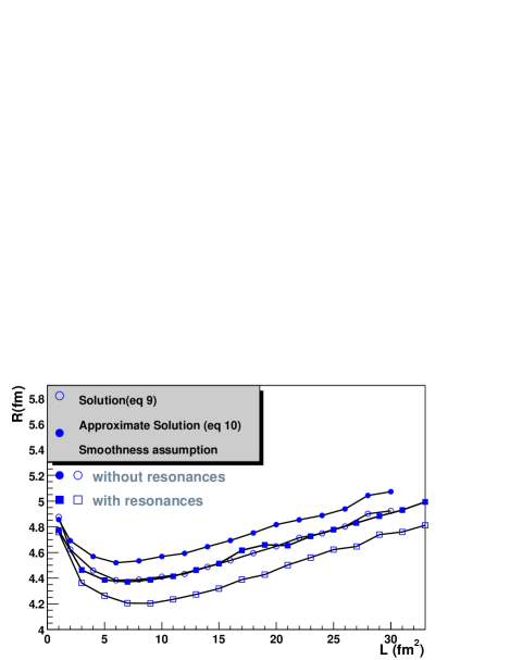
FIG. 16.: The apparent source radius R determined by $C({\bf k})=1+\lambda exp(-{4\bf k}^{2}R^{2})$ as a function of L including and excluding the pairs in which at least one pion comes from resonance decay

This result is understandable: at the late time when the resonances disintegrate there is no other particle close by and hence the value of $\mbox{${\bf q}$}\mbox{${\bf r}$}(t_{2})$ is large. On the average this contribution is therefore negligible.

VI correlation function of the kaons

So far we have investigated pions. In the simulation programs we have sufficient $K^{+}$ to allow for the calculation of a correlation function. The result is displayed in fig.17.

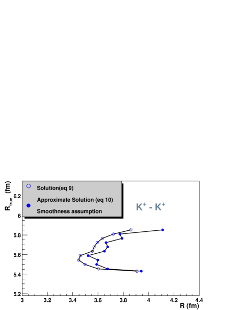
FIG. 17.: The true source radius $R_{true}$ (as given by the simulation program) for kaons as a function of the apparent source radius R determined by $C({\bf k})=1+\lambda exp(-{4\bf k}^{2}R^{2})$.

We observe a very similar behavior as for the pions because the space-momentum space correlations are similar. The kaon source is smaller than that of the pions: $R_{true}$ as well as R are smaller. The $K^{+}$ cross sections are lower and therefore the freeze out happens earlier. Consequently the smaller source radius is a natural consequence of known physics. We observe as well a large discrepancy between $R_{true}$ and R.

VII Conclusion

We studied in detail two problems which one encounters if one tries to interpret HBT correlation functions obtained from numerical simulations of heavy ion reactions at CERN energies: The influence of space - momentum space correlations and the influence of final state Coulomb interactions. For this purpose we supplemented one of the presently available programs, neXus, by electromagnetic interactions.

We find, first of all, that there is nothing like a static source which emits particles. The particles come from sources of quite different sizes because the system expands as a whole. Momenta and positions of the particles are strongly correlated and hence the source is not chaotic. Both observations render the task rather difficult to extract from the correlation function useful information on the size of the system or on densities. The most one can expect to obtain are a time averaged values. However, even these time averaged quantities are neither unique (different particle species give different values) nor representative (pairs of particles with small relative momenta (to which the correlation function is sensitive) are emitted from a smaller source then arbitrary pairs).

In order to calculate a correlation function in these semiclassical simulation programs one has to introduce (at least) one free parameter. Here we assume that the particles have a Gaussian wave function after their last collisions. Consequently, the simulation programs cannot predict the two body correlation functions. They can only determine for which variance the calculated two body correlation functions agrees with experiment.

Knowing the variance of the wave function and the freeze out points we can calculate in the simulation programs directly the average rms radius of the source. It is called $R_{true}$. All correlation functions we obtain have the form $C(\mbox{${\bf k}$})=1+\lambda e^{-4\mbox{${\bf k}$}^{2}R^{2}}$, the same form as seen in the experiments. Thus the crucial problem is to relate the apparent source radius R with physically meaningful quantities like $R_{true}$.

The simulation program tells us that there is no simple relation between R and $R_{true}$ due to four different reasons:

1) The distribution of the emission points is not Gaussian, whereas (due to the the finite error bars in the simulation as well as in the experiments) the correlation function is well described by a Gaussian and finer details of the source cannot be resolved in the correlation function. Therefore there is a difference between R and $R_{true}$ already of the order of 20%. Furthermore, the distribution of emission points and the distribution of sources (as displayed in fig.3) differ as well considerably. The latter is the relevant quantity if one would like to extract densities or energy densities.

2) For the reaction investigated the strong space-momentum space correlations modify the relation between R and $R_{true}$ in an important way. Thus R does not measured the true size of the source but underestimates it by $\approx 16\%$ and hence the true average density of the system is $60\%$ lower than that extract from R. This may explain the fact that the experimental source sizes, when analyzed under the assumption that the source is (almost) chaotic are incomprehensibly small. The relation between R and $R_{true}$ depends in a complicated way on the dynamics of the system and is not due to quantities like flow. Thus it is not evident how the information on space-momentum space correlations can be incorporated in more phenomenological approaches and, consequently, how this type of models can extract the true source radius from the observed apparent source radius.

3) The Coulomb interaction changes the relation between R and $R_{true}$ as well. Assuming that our calculation gives quantitatively reliable results, the difference between R and $R_{true}$ can reach $30\%$ and hence the densities differ by a factor of 2. For the influence of the Coulomb interaction we presented here only very approximative results. They are based on classical Coulomb trajectory calculations. They show that the Coulomb interaction between the correlated pairs and the other charges is as important as the Coulomb interaction between the particles of the correlated pair and that the standard procedure to use Gamow correction factors is not justified, because the average particle distance at freeze out is too large.

4) The difference between R and $R_{true}$ depends on the particle species because their cross section are different.

Thus this study shows that two problems have to be solved before the correlation function measurements can provide useful information on the density of the system. We have a) to understand how the apparent source radius is related to the time averaged true source radius and b) how the true source radius can be related to physical quantities like energy densities or densities. Here we have addressed the first question only and found that the difference between R and $R_{true}$ is all but negligible. Hence a naive interpretation of the observed apparent source radius as the radius of the system at freeze out is certainly premature.

The Coulomb interaction produces still another effect if one employs the standard method of event mixing because the absence of the Coulomb interaction in mixed events modifies the correlation function. This effect we have observed in the simulations but not discussed here. It will further add to the difficulty to relate the apparent source radius to the true source size.