About the parity-non-conserving asymmetry in $\vec{n}+p\rightarrow d+\gamma$

Abstract

The parity-non-conserving (pnc) asymmetry in $\vec{n}+p\rightarrow d+\gamma$ at thermal energies has recently been calculated using effective field-theory methods. A comparison of this calculation with much more elaborate calculations performed in the 70’s is made. This allows one to assess the validity of this new approach as presently used. It is found to overshoot the almost exact calculations by a factor close to 2 for the contribution involving the ${}^{3}S_{1}$ component of both the initial and final states. This is much larger than anticipated by the authors. This discrepancy is analyzed and found to originate from the over-simplified description of the deuteron and capture states which underlies the new approach. The claim that earlier determinations of the sign would be in error is also examined. It is found that the sign discrepancy is most probably due, instead, to the fact that the pion-nucleon interaction referred to by the authors corresponds to a parity-non-conserving potential with a sign opposite to what is currently used. Some estimates and constraints relative to the pnc $\pi$NN coupling, $h^{1}_{\pi}$, which the above asymmetry is dependent on, are reviewed. Further details are given in an Appendix.

1 Introduction

At the time where a new measurement of the parity-non-conserving (pnc) asymmetry in radiative neutron-proton capture at low energy is in preparation at LANSCE [1], intending to improve upon a previous one at ILL [2], it is appropriate to wonder about the validity of theoretical estimates of the effect. This one is expected to be dominated by the contribution of the pnc pion-exchange force and its measurement should therefore provide unique information on the pnc $\pi$NN coupling, $h^{1}_{\pi}$, which it strongly depends on. This coupling constant is an important ingredient of pnc NN forces and its determination represents a major goal in the field (see [3] for a review). This program supposes that theoretical uncertainties related to the description of the deuteron and np capture states are small enough so that the coupling can be reliably extracted from the measurement. By examining studies performed in the 70’s [4, 5, 6, 7] and later [8], some values with different signs and magnitudes can be found. Yet, it was concluded that the estimates of the asymmetry were rather independent of the strong interaction model [9] but not much detail was published on the relevance of some ingredients (see below). When correct ones are used, the relation between the pnc asymmetry to be measured, $A_{\gamma}$, and the above coupling, $h^{1}_{\pi}$, is essentially given by:

$$A_{\gamma}=-0.11\,h^{1}_{\pi}.$$

From the comparison of results obtained with reasonable strong interaction models, an uncertainty of about 5% could be ascribed to the above value. This one is slightly larger than the first estimate by Danilov [10], $A_{\gamma}=-0.08\,h^{1}_{\pi}$, which was obtained on the basis of an approach directly relying on nucleon-nucleon phase shifts, but neglecting the effect of the tensor force.

Recently, a new calculation based on a different approach, namely an effective field theory [11], came with a larger value, $A_{\gamma}=+0.17\,h^{1}_{\pi}$, and furthermore an opposite sign. An uncertainty of about 30% was ascribed to this value by the authors. This one could thus be compatible with the previous one, but it could also be twice as large. Apart from the fact that the discrepancy invalidates at first sight the argument that the coupling, $h^{1}_{\pi}$, could be determined unambiguously from the measurement of $A_{\gamma}$, it is important to determine how reliable is the new calculation and how it should be corrected when improvements are made. Notice that values of the asymmetry with a size comparable to the above one may be found in the literature but they correspond to a singlet scattering length inappropriate for the neutron-proton system.

The sign of the effect is another issue which deserves attention. It is the first information that one can hope to extract from an experiment, prior to the size itself. When calculations of the asymmetry $A_{\gamma}$ were performed in the early 70’s, it was believed that the sign of the pnc coupling, $h^{1}_{\pi}$, could not be determined theoretically, partly explaining the existence in the literature of relations of $A_{\gamma}$ to $h^{1}_{\pi}$ with different signs [9]. Since a theoretical determination of this sign has been made relatively to the parity conserving one, $g_{\pi NN}$, (this is the information that matters) [12], it is essential to establish what is the correct sign for the relation of $A_{\gamma}$ to $h^{1}_{\pi}$.

It this paper, we intend to compare the recent calculation to earlier ones, which, because they were quite sophisticated, can be used as a benchmark for testing the applicability of the effective field-theory methods to the process under consideration. At the same time, we discuss the points that are sources of discrepancy between calculations. After reminding a few ingredients required for the calculation of the pnc asymmetry of interest here, we show that the expression obtained in the new approach at the leading order identifies to a standard potential based calculation employing zero-range nucleon-nucleon forces (Sect. 2). In the third section, we discuss the size of the effect in relation with a better description of the nucleon-nucleon states. This is partly done by using analytical calculations, which has the advantage to show how the result changes while improvements are made. Section 4 is devoted to the sign of the effect. Details are given, allowing one to check its derivation. We, in particular, discuss the independence of this sign with respect to conventions that appear at intermediate steps of the calculation. In the fifth section, we present a short critical review of what is known, both theoretically and phenomenologically, on the elementary pnc $\pi$NN coupling constant, $h^{1}_{\pi}$. More details about this coupling are given in an Appendix.

2 Main ingredients entering the calculation of $h^{1}_{\pi}$

Due to parity-non-conservation in nucleon-nucleon forces, the emission of photons in the thermal neutron-proton capture can evidence an asymmetry with respect to the neutron polarization. This one, $A_{\gamma}$, is defined by the angular dependence of the capture cross section on the angle, $\theta$, between the direction of the photon emission and the neutron polarization, $W(\theta)\propto(1+A_{\gamma}\,{\rm cos}\,\theta)$. A simplified expression, which accounts for the dominant contributions of interest here, is given by:

$$A_{\gamma}=-2\;\frac{\tilde{E}1}{M1}.$$ (1)

In this formula, the factor 2 is a current one appearing in expressions for an asymmetry. The sign is well defined but supposes that appropriate conventions are used to calculate the matrix elements, $\tilde{E}1$ and $M1$. This will be detailed in the fourth section together with the spin-isospin algebra relative to the corresponding operators as well as to the pnc pion-exchange potential. The calculation of the two matrix elements are performed from the standard expressions for the electric and magnetic, $\Delta J=1$, transition operators. For the first one, we rely on the Siegert theorem, which allows one to sum up various contributions implied by gauge invariance, including those pertaining to the description of the pnc interaction. The sign difference which depends on whether the photon is absorbed or emitted is taken care of. For simplicity, factors that cancel out in the ratio given by Eq. (1) are ignored.

The matrix element $M1$ of interest here involves the overlap of the wave functions of the deuteron state and the ${}^{1}S_{0}$ scattering state, which is the dominant one and provides most of the contribution to the capture cross section. It is given by:

$$M1=(\frac{\mu_{p}-\mu_{n}}{2M_{N}})\;\int dr\,r^{2}\;\psi_{d}(r)\,\psi_{s}(r).$$ (2)

The matrix element, $\tilde{E}1$, involves a transition between the deuteron state and the ${}^{3}S_{1}$ scattering state. Its value, which is zero if parity is conserved, depends on the odd-parity component admixed to either state by the pnc nucleon-nucleon force. Capture from the ${}^{3}S_{1}$ state is not large, but it appears here because a state with a polarized neutron necessarily results from its coherent superposition with a ${}^{1}S_{0}$ state. The expression of the matrix element is given by:

$$\tilde{E}1=\frac{1}{3}\,\int dr\,r^{2}\;\left(\psi_{d}(r)\,r\,\tilde{\psi}_{t}(r)-\tilde{\psi}_{d}(r)\,r\,\psi_{t}(r)\right),$$ (3)

where the factor $\frac{1}{3}$ comes from integrating over angles the angular dependence due to both the dipole operator and the parity admixed component with the result

$$\int\frac{d\Omega}{4\pi}\,r^{i}r^{j}=\,\frac{1}{3}\,r^{2}\,\delta^{ij}.$$

The minus sign in Eq. (3) comes from taking the complex conjugate of the complete deuteron wave function whose parity admixture contains the extra imaginary number, i (which combines with a i in the electric dipole operator to produce a real number). For simplicity, the admixture of a ${}^{3}D_{1}$ component to the ${}^{3}S_{1}$ one has been omitted in the above equation (as it was in [11]) but it is accounted for in the most elaborate calculations whose results are reminded below. For the calculation of interest here, its effect can be accounted for by replacing the current ${}^{3}S_{1}$-wave component, $u(r)$, by the combination involving the D-wave component, $u(r)+\frac{1}{\sqrt{2}}\,w(r)$. As to the quantities, $\tilde{\psi}_{d}(r)$ and $\tilde{\psi}_{t}(r)$, they respectively describe the parity admixed components to the deuteron and the ${}^{3}S_{1}$ scattering states. As shown by Danilov [10], these components involve a pnc transition from a ${}^{3}S_{1}$ to a ${}^{3}P_{1}$ state (the electric dipole operator does not change the spin for its dominant contribution) and, thus, implies a $T=0$ to a $T=1$ transition. This can only arise from an isovector pnc force.

The isovector pnc force is expected to be largely dominated by the pion-exchange contribution, due to the relatively low mass of the pion and, consequently, its somewhat long range. The expression for this force, first given in [13], is currently written down as follows [14, 15, 3]:

$$V_{\pi}=i\,\frac{g_{\pi NN}\,h^{1}_{\pi}}{2\sqrt{2}}\;(\vec{\tau}_{1}\times\vec{\tau}_{2})^{z}\,(\vec{\sigma}_{1}+\vec{\sigma}_{2})\left[\frac{\vec{p}_{1}-\vec{p}_{2}}{2M_{N}},\frac{e^{-m_{\pi}r}}{4\pi\,r}\right],$$ (4)

where $g_{\pi NN}$ represents the strong $\pi$NN coupling constant, which is taken positive here as usually done. Contrary to the meson-nucleon interaction, the above expression of the pnc potential is essentially free of any convention. The sign of $V_{\pi}$ is therefore determined by the sign of $h^{1}_{\pi}$ (see Sect. 4 for more details).

Knowing the expression of the pnc force, one can now determine the parity admixed components it produces in the total deuteron or ${}^{3}S_{1}$ scattering states, which we write as:

$$|\Psi>_{d,t}=\left(\psi_{d,t}(r)+...+i\,\frac{\tau^{z}_{p}-\tau^{z}_{n}}{2}\,(\vec{\sigma}_{p}+\vec{\sigma}_{n}).\frac{\vec{r}_{p}-\vec{r}_{n}}{|\vec{r}_{p}-\vec{r}_{n}|}\,\tilde{\psi}_{d,t}(r)\right)|S=1>,$$ (5)

where the dots stand for the tensor component we omit for simplicity. From now on, particles 1 and 2 are ascribed to the proton and neutron respectively, but we nevertheless keep track of the isospin factor, equal to 1, to evidence the symmetry between the two particles. As the pnc force is a small perturbation, the expressions of the parity admixed components, $\tilde{\psi}_{d}(r)$ and $\tilde{\psi}_{t}(r)$, can be obtained using the full Green’s function projected on $l=1$ angular momentum states. For the deuteron state, one gets:

$$\tilde{\psi}_{d}(r)=\int dr^{\prime}\,r^{\prime 2}\;G^{l=1}_{E}(r,r^{\prime})\frac{g_{\pi NN}\,h^{1}_{\pi}}{4\pi M_{N}\sqrt{2}}\;\frac{e^{-m_{\pi}r^{\prime}}}{r^{\prime 2}}(1+m_{\pi}r^{\prime})\;(\psi_{d}(r^{\prime})+...),$$ (6)

where $E=-|E_{d}|$. A similar expression holds for the scattering state with the appropriate replacements. Spin and isopin dependences have been factored out so that Exp. (1) (together with Exps. (2, 3, 6)) offers no ambiguity as to its sign once the sign of $h^{1}_{\pi}$ is given (intrinsic phases relative to the deuteron or scattering states cancel out).

A first but unrealistic estimate of the asymmetry, $A_{\gamma}$, can be obtained by using the following wave functions corresponding to a zero-range force together with the free Green’s function projected on the $l=1$ space:

$$\psi^{0}_{s}(r)=1-\frac{a_{s}}{r},\;\;\;\;\psi^{0}_{t}(r)=1-\frac{1}{\alpha r},\;\;\;\;\psi^{0}_{d}(r)=\sqrt{2\alpha}\;\frac{e^{-\alpha r}}{r},$$ (7)

$$G^{l=1}_{E=0}(r,r^{\prime})=-M_{N}\,\frac{1}{\,r^{2}}\,\left(\frac{r^{\prime}}{3}\;\;\theta(r-r^{\prime})\right)+...,\hskip 142.26378pt$$

$$G^{l=1}_{E=-|E_{d}|}(r,r^{\prime})=-M_{N}\,\frac{e^{-\alpha r}\,(1+\alpha r)}{r^{2}}\hskip 184.9429pt$$

$$\left(\frac{e^{-\alpha r^{\prime}}\,(1+\alpha r^{\prime})-e^{\alpha r^{\prime}}\,(1-\alpha r^{\prime})}{2\alpha^{3}\,r^{\prime 2}}\;\;\theta(r-r^{\prime})\right)+....$$ (8)

In these equations, $\alpha$ is related to the deuteron binding energy, $\alpha=\sqrt{M_{N}|E_{d}|}$. The expression of the Green’s function, only given for $r^{\prime}<r$, allows one to precise factors.

The calculation of integrals in Eqs. (2, 3, 6) can be performed analytically with the result:

$$A^{0}_{\gamma}=-\frac{g_{\pi NN}\,h^{1}_{\pi}\,M_{N}\sqrt{2}}{3\pi\,(\mu_{p}-\mu_{n})(1-\alpha a_{s})}\left[\frac{m_{\pi}}{(m_{\pi}+\alpha)^{2}}+\frac{m_{\pi}^{2}}{\alpha^{2}(m_{\pi}+\alpha)}-\frac{m_{\pi}^{2}}{2\alpha^{3}}\,{\rm log}(1+\frac{2\alpha}{m_{\pi}})\right].$$ (9)

This expression is identical to that one obtained by Kaplan et al. when using the effective field theory at the leading order. In view of the extreme simplicity of the wave functions it corresponds to, the result can be easily improved. By using more realistic wave functions, one can provide insight on the corrections that should be applied to the estimate of $A_{\gamma}$ made by these authors. Let’s notice that, due to different inputs concerning mainly the strong $\pi NN$ coupling, the magnitude of the asymmetry given by the above equation is slightly larger than what they obtain. The discrepancy has not much physical relevance but is important in order to assess the precise validity of the approach. Thus, the value to be compared with more elaborate estimates presented below is $-0.187\,h^{1}_{\pi}$ (corresponding to $\frac{g^{2}_{\pi NN}}{4\pi}=14.4,\,m_{\pi}=0.7\,{\rm fm}^{-1},\,M_{N}=4.76\,{\rm fm}^{-1},\,\mu_{p}-\mu_{n}=4.706,\,\alpha=0.232\,{\rm fm}^{-1},\,a_{s}=-23.7\,$fm).

3 Size of the effect

The size of the pnc asymmetry, $A_{\gamma}$, has been calculated in many papers [10, 4, 5, 6, 7, 8]. They evidence discrepancies depending on whether results are corrected for the fact that most realistic models used in the past were not providing the right neutron-proton scattering length for the ${}^{1}S_{0}$ state. These models were assuming isospin symmetry, often predicting a scattering length of about $-17\,$fm. This represents the main source of difference, roughly a factor 1.4 ($\simeq\frac{-23.7}{-17}$). Actually, this can be remedied by taking the value of the regular transition amplitude, $M1$, from the measured capture cross section, which offers the further advantage to also account for a 5% correction due to meson-exchange currents. Results also depend on whether interaction in P waves or effects due to the tensor force are considered. When the main ingredients mentioned above are accounted for [9], the uncertainty is due to the strong interaction models themselves and the precise way to correct for their deficiencies. Asymmetries calculated on the same footing with the Hamada-Johnston, Reid-soft-core and de Tourreil-Sprung potential models for instance were found to be equal to $-0.109\,h^{1}_{\pi}$, $-0.114\,h^{1}_{\pi}$ and $-0.107\,h^{1}_{\pi}$ respectively [5]. In all cases, the effect of the repulsion in the ${}^{3}P_{1}$ state ($\simeq 25-30\%$) is partly compensated by an effect of about 20% due to the admixture of a ${}^{3}D_{1}$ component to the ${}^{3}S_{1}$ one. Careful examination also indicates that part of the differences has a well determined origin: a slightly too large binding energy for the deuteron in the case of the Hamada-Johnston model and a 2% difference for the triplet scattering length for the two other models. The discrepancies can therefore be made smaller by using improved models of the NN interaction.

The insensitivity to the strong interaction model was confirmed later on by using the Paris potential [8], which is a more up to date model, including an accurate treatment of the two pion-exchange contribution. Prior to the comparison, the result has to be corrected for a wrong ${}^{1}S_{0}$ scattering length however.

The above values have a magnitude smaller than what was obtained by Kaplan et al., $-0.187\,h^{1}_{\pi}$ with our inputs (see remark end of previous section). The discrepancy can be easily ascribed to the oversimplified wave functions, which the Kaplan et al.’s calculation corresponds to (Eq. 9). With respect to these ones, Hulthén wave functions (corresponding to a separable Yamaguchi potential) represent a significant improvement although they are not good ones in view of the present standard. They offer the advantage of providing an analytic expression for the pnc asymmetry, $\tilde{E}1$, which can be used to estimate the effect of the finite range of the strong interaction neglected in the above calculation. It is given by:

$$A^{1}_{\gamma}=-\frac{g_{\pi NN}\,h^{1}_{\pi}\,M_{N}\sqrt{2}}{3\pi\,(\mu_{p}-\mu_{n})\;\left(1-(\frac{\alpha}{\eta_{t}})^{2}-\alpha a_{s}(1-\frac{\alpha}{\eta_{t}}-\frac{\alpha}{\eta_{s}+\alpha}+\frac{\alpha}{\eta_{s}+\eta_{t}})\right)}\hskip 113.81102pt$$

$$\times\left[\frac{m_{\pi}}{(m_{\pi}+\alpha)^{2}}+\alpha a_{t}\,\left(\frac{m_{\pi}^{2}}{\alpha^{2}(m_{\pi}+\alpha)}-\frac{m_{\pi}^{2}}{2\alpha^{3}}\,{\rm log}(1+\frac{2\alpha}{m_{\pi}})\right)\right.\hskip 113.81102pt$$

$$\left.-\frac{m_{\pi}}{(m_{\pi}+\eta_{t})^{2}}-\frac{\eta_{t}^{2}-\alpha^{2}}{2\eta_{t}(m_{\pi}+\eta_{t})^{2}}\right.\hskip 227.62204pt$$

$$\left.-\alpha a_{t}\left(\frac{2m_{\pi}^{2}-2\eta_{t}^{2}-\alpha m_{\pi}+\alpha\eta_{t}}{4\alpha^{2}(m_{\pi}+\eta_{t})}+\frac{2m_{\pi}^{2}-2\eta_{t}^{2}+\alpha m_{\pi}-\alpha\eta_{t}+\alpha^{2}}{4\alpha^{2}(m_{\pi}+\eta_{t}+\alpha)}\right.\right.\hskip 85.35826pt$$

$$\left.\left.-\frac{2m_{\pi}^{2}-2\eta_{t}^{2}+\alpha^{2}}{2\alpha^{3}}{\rm log}(\frac{m_{\pi}+\eta_{t}+\alpha}{m_{\pi}+\eta_{t}})\right)\right.\hskip 142.26378pt$$

$$\left.+\frac{\alpha^{2}a_{t}}{(\eta_{t}+\alpha)^{2}}\left(\frac{2m_{\pi}^{2}+\eta_{t}^{2}+m_{\pi}\eta_{t}-\alpha m_{\pi}-\alpha^{2}}{4(\eta_{t}-\alpha)(m_{\pi}+\eta_{t}+\alpha)}-\frac{m_{\pi}^{2}}{2(\eta_{t}-\alpha)^{2}}{\rm log}(\frac{m_{\pi}+\eta_{t}+\alpha}{m_{\pi}+2\alpha})\right)\right.\hskip 28.45274pt$$

$$\left.-\frac{\alpha^{2}a_{t}}{\eta_{t}^{2}}\left(\frac{2m_{\pi}^{2}+\eta_{t}^{2}+m_{\pi}\eta_{t}}{4\eta_{t}(m_{\pi}+\eta_{t})}-\frac{m_{\pi}^{2}}{2\eta_{t}^{2}}{\rm log}(\frac{m_{\pi}+\eta_{t}}{m_{\pi}})\right)\right.\hskip 85.35826pt$$

$$\left.-\frac{\alpha^{2}a_{t}}{(\eta_{t}+\alpha)^{2}}\left(\frac{2m_{\pi}^{2}-2\eta_{t}^{2}+m_{\pi}\eta_{t}-\alpha m_{\pi}+2\alpha\eta_{t}}{4(\eta_{t}-\alpha)(m_{\pi}+2\eta_{t})}-\frac{m_{\pi}^{2}-\eta_{t}^{2}+\alpha^{2}}{2(\eta_{t}-\alpha)^{2}}{\rm log}(\frac{m_{\pi}+2\eta_{t}}{m_{\pi}+\eta_{t}+\alpha})\right)\right.$$

$$\left.+\frac{\alpha^{2}a_{t}}{\eta_{t}^{2}}\left(\frac{2m_{\pi}^{2}-2\eta_{t}^{2}+m_{\pi}\eta_{t}}{4\eta_{t}(m_{\pi}+2\eta_{t})}-\frac{m_{\pi}^{2}-\eta_{t}^{2}}{2\eta_{t}^{2}}{\rm log}(\frac{m_{\pi}+2\eta_{t}}{m_{\pi}+\eta_{t}})\right)\right].\hskip 85.35826pt$$ (10)

In the limit of a zero-range force ($\eta_{t}\rightarrow\infty,\,\alpha a_{t}\rightarrow 1$), the front factor together with the first line in the above equation allow one to recover Eq. (9), while the other terms vanish as $\eta_{t}^{-1}$ or $\eta_{t}^{-2}$. For the value that $\eta$ is expected to take in the case of a finite range force ($\eta_{t}=1.386\,{\rm fm}^{-1}$ corresponding to $a_{t}=5.42\,{\rm fm}$ and $\alpha=0.232\,{\rm fm}^{-1}$, and $\eta_{s}=1.203\,{\rm fm}^{-1}$), one gets a reduction by a factor 1.33.

Another analytical estimate of the effect can be obtained using the Danilov’s approach [10]. This one, which relies on dispersion relations, only uses the knowledge of NN scattering phase shifts. It has been shown to give a good account of pnc effects in the neutron-proton radiative capture process, the uncertainty being of the order of 20-25% in absence of accidental cancellation [16]. In this approach, the whole effect is factorized into two parts involving the electric dipole operator and the pnc NN force, which respectively are sensitive to the long and medium plus short range description of NN states. The pnc effect is thus determined by the strength of the pnc neutron-proton scattering amplitude, $M_{N}C$, whose expression is given by:

$$M_{N}C=-\frac{g_{\pi NN}\,h^{1}_{\pi}}{4\pi\sqrt{2}}\frac{M_{N}}{a_{t}}F_{t}(0)\;\int_{-\infty}^{-\frac{m^{2}_{\pi}}{4}}dp^{\prime 2}\;(-\frac{m^{2}_{\pi}}{8\,p^{\prime 6}})\;F^{-1}_{t}(p^{\prime 2}).$$ (11)

where

$$F^{-1}_{t}(p^{2})=(1+\frac{p^{2}}{\alpha^{2}})\;\;{\rm exp}\left(\frac{p^{2}}{\pi}\int_{0}^{\infty}\frac{dp^{\prime 2}(\delta_{t}(p^{\prime 2})-\pi)}{p^{\prime 2}\,(p^{2}-p^{\prime 2}+i\epsilon)}\right),\;\;(\delta(0)=\pi).$$ (12)

Inserting in this equation the standard low energy effective range parametrization for phase shifts, $\frac{p}{{\rm tg}\,\delta_{t}}=-\frac{1}{a_{t}}+\frac{r_{t}\,p^{2}}{2}$, one gets:

$$F^{-1}_{t}(p^{2})=\frac{1-\frac{\sqrt{-p^{2}}}{\alpha}}{1+\frac{\alpha a_{t}r_{t}\sqrt{-p^{2}}}{2}}\;\;({\rm for}\,p^{2}<0),$$ (13)

and from it:

$$M_{N}C = -\frac{g_{\pi NN}\,h^{1}_{\pi}}{4\pi\sqrt{2}}\frac{M_{N}}{a_{t}}\int_{\frac{m_{\pi}}{2}}^{\infty}dq\,\frac{m^{2}_{\pi}}{4\,q^{5}}\,\frac{1-\frac{q}{\alpha}}{1+\frac{\alpha a_{t}r_{t}\,q}{2}}$$

$$= \frac{g_{\pi NN}\,h^{1}_{\pi}}{4\pi\sqrt{2}}\frac{M_{N}}{\alpha a_{t}m_{\pi}}\left((1+\frac{2\alpha}{m_{\pi}}\,x)(\frac{2}{3}-x+2x^{2}-2x^{3}{\rm log}(1+\frac{1}{x}))-\frac{\alpha}{m_{\pi}}\right),$$

with $x=\frac{\alpha\,a_{t}\,r_{t}\,m_{\pi}}{4}$. A numerical estimate of the effect of the range is immediately obtained by comparing values of $M_{N}C$ calculated with $r_{t}=\,1.765\,$fm and $r_{t}=\,0$. A reduction by a factor 1.6 is thus found in the case of the scattering state. This is partly reduced by the fact that the scattering length $a_{t}$ is simultaneously enhanced, the real reduction factor being closer to 1.3.

The apparent independence of expressions (11-14) of strong interaction models (it is sufficient to know the phase shifts) is partly misleading. It is likely that the off-shell effects that the underlying approach neglects have to be accounted for by extra contributions to the dispersion relation, Eq. (11).

Estimates due to a better description of the S states given above do not take into account the repulsion at short distances. From the comparison with results from realistic NN interaction models, an extra reduction by a factor $\simeq 1.15-1.20$ is found for this part. Some reduction by a factor $\simeq 1.25-1.30$ is also due to the repulsion in the ${}^{3}P_{1}$-state. Thus the total reduction of $A_{\gamma}$ with respect to the value $-0.187\,h^{1}_{\pi}$ amounts to a factor $\simeq 1.9-2.0$. The size of the effect is larger than the 30% referred to in ref. [11]. With this respect, we would like to mention that this uncertainty is almost reached by the effect of neglecting the finite range of the interaction. The value of the product $\alpha\,a_{t}$, which is set to 1 in the zero-range limit, is actually larger by a factor 1.26. The deuteron asymptotic normalization, $\sqrt{2\alpha}$, is found smaller than the experimental one, 0.884 fm${}^{-\frac{1}{2}}$ by a factor 1.30. As these discrepancies concern long range properties, one should not be surprised by the significantly larger discrepancy we found for the pnc effect. This one depends on the short range properties that are much less well described by the present use of effective field-theory methods.

The agreement obtained for the total capture cross section was considered by Kaplan et al. as a support for their approach [11]. In view of the previous comments, it looks somewhat accidental. It results from a cancellation of two effects: a long range contribution that is too small and a shorter range contribution (further enhanced for the pnc case) that is too large.

4 Sign of the effect

Signs in the field of parity violation are an important information but have not always received the attention they deserve. The size of the measured pnc asymmetry in pp scattering at low energy has been reproduced in many papers for instance. A careful examination nevertheless showed that ten of them were actually missing the sign [17]. In view of this, we here precise ingredients that enter into the determination of the sign of the pnc asymmetry, $A_{\gamma}$, together with its expression. They concern the pnc potential, $V_{\pi}$, the electromagnetic transition operators, and the calculation of the asymmetry itself.

The determination of the sign of the pion-exchange pnc force, Eq. (4), has been made for the first time in ref. [12]. It makes sense as far as the expression of Pauli matrices and the relation $\vec{p}=-i\vec{\nabla}$ are universally accepted. The sign is then related to the sign of the product of the strong and weak $\pi$NN couplings. Individually, the sign of each of them depends on many conventions: intrinsic phase of the meson field, definition from an Hamiltonian or from a Lagrangian, expression of the $\gamma$ matrices, especially the $\gamma_{5}$ matrix which makes the difference between a pc and a pnc interaction, spin-$\frac{1}{2}$ fields referring to particles or anti-particles, metric, … While it is possible to get rid of all these conventions with some care, this is not sufficient to determine the sign of the product of the couplings. The last step is achieved by noticing that the calculation of the pnc coupling, $h^{1}_{\pi}$, using PCAC and current algebra, is involving a factor proportional to the strong coupling, hence a dependence of $g_{\pi NN}\,h^{1}_{\pi}$ on the quantity $g^{2}_{\pi NN}$, which is always positive [12]. The sign of the three types of contributions considered in DDH (sum rule, “parity admixture” into the wave function and factorization; see Fig. 1c, 1b, 1a in the Appendix) could thus be determined. Taking as positive the strong coupling appearing in the pnc potential, Eq. (4), as done in DDH and subsequent papers [14, 3], the estimated weak coupling $h^{1}_{\pi}$ and its range given in these works correspond to a positive value.

The electric $E1$ and magnetic $M1$ operators are a possible source of sign mistake. They can be derived from the electromagnetic Hamiltonian, which may be written as:

$$H_{el}=e\sum_{j}\left((\frac{(\vec{p}_{i}+\vec{p}_{f})\,.\,\vec{\epsilon}}{2\,M_{N}})_{j}\,(\frac{1+\tau^{z}}{2})_{j}\pm i(\frac{\mu_{p}}{2M_{N}}\,\frac{1+\tau^{z}}{2}+\frac{\mu_{n}}{2M_{N}}\,\frac{1-\tau^{z}}{2})_{j}\;\vec{\sigma}_{j}\,.\,\vec{q}\times\vec{\epsilon}\,\right)+...$$ (15)

where the dots account for meson-exchange currents required to ensure gauge invariance. The photon polarization is represented by the vector $\vec{\epsilon}$ and its momentum (energy) by $\vec{q}\,(q^{0})$. An alternative expression, which is of more direct usefulness for the present work, relies on the Siegert theorem to account for the dominant contributions due to exchange currents (represented by dots below),

$$\sum_{j}(\frac{\vec{p}\,.\,\vec{\epsilon}}{2\,M_{N}})_{j}\,(\frac{1+\tau^{z}}{2})_{j}+....=i\,\frac{1}{2}\,\left[H_{pc}+H_{pnc},\sum_{j}\vec{r}_{j}\,(\frac{1+\tau^{z}}{2})_{j}\right].$$

It is given by:

$$H_{el}=e\left(\pm i\,\frac{1}{2}\,q^{0}\,(\vec{r_{p}}-\vec{r_{n}}).\vec{\epsilon}\pm i\,\frac{1}{2}\,\frac{\mu_{p}-\mu_{n}}{2M_{N}}(\vec{\sigma_{p}}-\vec{\sigma_{n}})\,.\,\vec{q}\times\vec{\epsilon}\right)\,\frac{\tau^{z}_{p}-\tau^{z}_{n}}{2}+....$$ (16)

where the dots, here and below, represent contributions that are irrelevant for our purpose. Different signs appear in Eq. (16) as well as Eq. (15), depending on whether an absorption or an emission of the photon is considered (or on whether one calculates the matrix element $<i|H|f>$ or $<f|H|i>$). The present ones are given for an emission (radiative capture) and respectively correspond to $<i|H|f>\;(<np|H|d\gamma>)$ and $<f|H|i>\;(<d\gamma|H|np>)$ for the upper and lower sign. Either way leads to the same result, but we nevertheless emphasize the point as the electric dipole operator, $\vec{r}$, in Eq. (16) has not always been used with the appropriate sign for the energy factor $q^{0}$, giving rise to different signs for the parity violating asymmetries [5, 9].

Using the expression of the electromagnetic interaction, Eq. (16), the expression of the total wave function, Eq. (5), together with Eq. (6) for the parity admixed component, one obtains the transition matrix operator in terms of the matrix elements, $M1$ and $\tilde{E}1$, previously defined, Eqs. (2, 3):

$$T(n\,p\rightarrow d\,\gamma)\propto\left(\pm i\,M1\,\,(\vec{\sigma_{p}}-\vec{\sigma_{n}})\,.\,\vec{q}\times\vec{\epsilon}+\tilde{E}1\,(\vec{\sigma_{p}}+\vec{\sigma_{n}})\,.\,(q^{0}\,\vec{\epsilon}-\vec{q}\,\epsilon^{0})+....\right).$$ (17)

The last term has been completed with a contribution from the charge density so that to emphasize its gauge invariance. Using the relation, $i\,(\vec{\sigma_{p}}-\vec{\sigma_{n}})=(\vec{\sigma_{p}}\times\vec{\sigma_{n}})\;P_{\sigma}$, one obtains an alternative expression. Less dependent on conventions as far as the relative sign of $M1$ and $\tilde{E}1$ contributions is concerned, it is given by:

$$T(n\,p\rightarrow d\,\gamma)\propto\left(M1\,(\vec{\sigma_{p}}\times\vec{\sigma_{n}})\,.\,\vec{q}\times\vec{\epsilon}+\tilde{E}1\,(\vec{\sigma_{p}}+\vec{\sigma_{n}})\,.\,(q^{0}\,\vec{\epsilon}-\vec{q}\,\epsilon^{0})+....\right).$$ (18)

The angular distribution of the emitted photons with respect to the neutron polarization $\vec{n}$ is obtained by taking the matrix element of the transition operator, $T$, corresponding to a given neutron polarization along this direction, multiplying it by its complex conjugate and summing over all polarizations in the final states. This amounts to calculate:

$$\sigma(\theta)\propto\sum_{\epsilon}{\rm Tr.}\;(\;(\frac{1+\vec{\sigma_{n}}.\vec{n}}{2})\;\;T\;\;(\frac{3+\vec{\sigma_{p}}.\vec{\sigma_{n}}}{4})\;\;T^{+}\;)$$

$$\propto(M1^{2}\,-2\;M1\;\tilde{E}1\;\;\vec{n}.\hat{q}+...),$$ (19)

from which Eq. (1) immediately follows.

5 Present estimates and constraints for the pnc coupling, $h^{1}_{\pi}$

There are in the literature numerous papers dealing with the estimate of the pnc coupling, $h^{1}_{\pi}$, in the standard electro-weak interaction model [18, 12, 19, 14, 20, 21, 22, 23, 24, 25, 26]. The most comprehensive work is still probably the DDH one [14]. Contributions considered since then most often correspond to one of those estimated in this earlier work. While the improvement is not always obvious, at least, they provide a better estimate of the uncertainty that should be ascribed to each of them. Due to expected cancellations between different contributions, picking up one of them is however misleading. Some details and a discussion are given in ref. [3] as well as in the Appendix. One of the features evidenced by the results, summarized in DDH, was their strong dependence on the factor, K, that accounts for strong interaction effects. Since then, due to improvements in determining the strong QCD coupling, the value of K has decreased from $K=6$ to $K=3$ for an energy scale of $\mu=1\,$GeV. It was also realized that there was some cancellation between the effect due to a dependence of the K factor on this (arbitrary) energy scale and that one for the quark masses [27], with the result of making estimates of pnc meson-nucleon couplings less dependent on it, as it should be. The introduction of a contribution implying strange quarks in the nucleon could have the same effect for another contribution involving strange quarks in the hadronic weak interaction. Thus, an up-dated range for the coupling would now be: $0<h^{1}_{\pi}<2.5\,10^{-7}$ (see [28] for an analysis of some uncertainties). Due to large cancellations in the total contribution involving u and d quarks (see Table 4 of ref. [3] and Appendix), most of the contribution arises from the part of the weak interaction involving strange quarks. It is interesting to notice that a recent estimate of the same contribution [26] falls in the above range. Other estimates fall outside. While that one for the strange quark in ref. [25] is not a serious source of concern in view of its very rough character, those based on QCD sum rules [20, 23, 24], which in any case ignore strange quarks, are. It is not clear which contribution they correspond to in the DDH picture. Let’s finally mention that all studies give positive values for $h^{1}_{\pi}$. From the examination of the papers however, we did not get the certitude that the sign was carefully determined (assuming it was looked at).

Phenomenological constraints on the coupling, $h^{1}_{\pi}$, have been recently discussed in the literature [3, 29]. To explain the recent measurement of the anapole moment in ${}^{133}Cs$ [30], it has been suggested that a large value of the coupling would be required [31, 32], exceeding the upper limit determined from the experiment performed at ILL in the past [2] ( $h^{1}_{\pi}=(1.4\pm 4.4)\,10^{-7}$, in absence of other contribution). An isoscalar pnc force enhanced in the nuclear medium could do as well with a coupling that would be smaller and essentially in agreement with what the absence of observed effect in ${}^{18}F$ indicates, $h^{1}_{\pi}\leq 1.3\,10^{-7}$ [3]. It is remembered that the calculation of the nuclear pnc matrix element in this case can be checked by using information from first forbidden $\beta$ decay from ${}^{18}Ne$. Although it has not the same probing strength as in ${}^{18}F$, the absence of effect in ${}^{21}Ne$ and in ${}^{93}Tc$ also points to a small coupling if one discards it results from accidental cancellations [3, 33]. Let’s remind that the present theoretical contribution of the pion-exchange to the circular polarization of photons emitted in the transition, $\frac{1^{-}}{2}\rightarrow\frac{3^{+}}{2}$ in ²¹Ne is expected to be about $|P^{\pi}_{\gamma}|=10^{5}\,|h^{1}_{\pi}|$, whereas the measurement puts the limit $P_{\gamma}=(0.8\pm 1.4)\times 10^{-3}$.

6 Conclusion

We have shown that, far from representing a progress, the recent calculation of the pnc asymmetry in $\vec{n}+p\rightarrow d+\gamma$, based on using effective field-theory methods at leading order, is a step back to pre-historic times of the field. While this approach looks appealing at first sight, it evidences large discrepancies with previous calculations. Realizing that these latter rely on much more elaborate descriptions of the deuteron and scattering states, they can be used to assess the validity of the new approach as used until now.

From the comparison we made, the uncertainty of 30% ascribed to it by the authors is reasonable for the calculation of observables that have a long range, such as magnetic or electric transitions. In the present case however, part of the effect involves a weak pnc interaction which has a shorter range. Examination of their expression for the asymmetry $A_{\gamma}$, which corresponds to an attractive zero-range force, shows that it behaves like $\frac{1}{m_{\pi}}$, while for reasonable potentials one rather expects $\frac{1}{m_{\pi}^{2}}$ (all other quantities being supposed to be small). This part of the calculation is overestimated by a factor of about 2. The discrepancy has its origin in the treatment of nucleon-nucleon correlations and especially their well known short range repulsive part, which prevents two nucleons to have an infinite probability to be close to each other (phase space factor put apart) as the present calculation by Kaplan et al. supposes. It decomposes into a factor roughly given by $(1+c\,\frac{r_{t}\,m_{\pi}}{3})\simeq 1.5-1.6$, representing the combined effect of a finite range attraction together with a short range repulsion for the force in the ${}^{3}S_{1}$ state ($r_{t}$ represents the effective range and $c\simeq 1.3$) and a factor $\simeq 1.25-1.30$ representing the effect of long and short range repulsion in the ${}^{3}P_{1}$ states. The overestimate is actually smaller by a factor $\simeq 1.15$ due to a contribution from the tensor force that is constructive in the present case, itself reduced by the correction of mesonic exchange currents to the regular transition, M1. While the new result by Kaplan et al. lets hope that the pnc asymmetry, $A_{\gamma}$, could be quite large in view of the error ascribed to the theoretical method, it thus appears that: 1) the error with respect to the actual value is underestimated, 2) this value is slightly outside the range they provided, in the lower part.

The underestimate of the error indicates that the parameter which, in the approach, governs the expansion at different orders does not provide a good magnitude of their relative contributions. This conclusion is supported by the omission of the dominant contribution to the deuteron anapole moment in [34] (corrected in [35]) which suggests that the determination of what is relevant at some order is not so straightforward. This does not preclude the use of effective approaches for describing pnc effects however. Such approaches were initiated in the field by Danilov with a different foundation [10] and extented to nuclei in [9]. They can give a good account of pnc effects in a large variety of low energy processes.

The determination of the sign of the asymmetry requires some care, especially to get rid of numerous conventions that appear at different steps of the calculation. Assuming that the authors of ref. [11] have relied on commonly used definitions for writting down the expression of the pion-nucleon coupling, we found that the pion-exchange potential which it gives rise to has a sign opposite to the current one, thus producing an asymmetry with the sign different from that one generally referred to. After correcting their result for this different choice, the determination of the sign by these authors confirms the earlier determination, thus providing the independent check that they were calling for.

Concluding, there is a long way ahead before the effective field-theory approach to the calculation of the asymmetry $A_{\gamma}$ be able to compete with more elaborate calculations. For the pion-exchange contribution, these ones converge to the value $A_{\gamma}=-(0.11\pm 0.01)\,h^{1}_{\pi}$. The sign refers to the current expression of the $\pi$-exchange pnc potential and the error, estimated largely, results from the comparison of the most realistic descriptions of the process.

Appendix: More about $h^{1}_{\pi}$

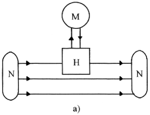
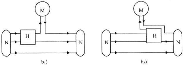
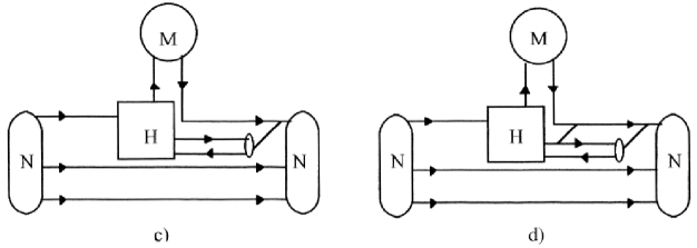
Figure 1: Quark processes contributing to the pnc meson-nucleon couplings. Diagrams labelled a, b, c, d, arise respectively from the factorization approximation, parity admixture into the nucleon, first order and part of the second order sea quarks. Diagram c) has been corrected with respect to the one presented in Ref. [3]. In all diagrams, the box represents the pnc quark interaction. Its effective character can be seen from the examination of the last two diagrams. By extending the box, it is possible to have it to incorporate that part involving gluon exchange so that to get a diagram a) type. On the other hand, the $\bar{q}q$ pair, which the gluon couples to, contains in particular a $\bar{s}s$ pair, colored in c), partly uncolored in d). This last diagram involves a sub-diagram similar to that one responsible for reducing the contribution of quarks to the nucleon spin.

Details on the theoretical estimates of the pnc coupling constant, $h^{1}_{\pi}$, are given here. As well known, this coupling depends on the isovector part of the hadronic weak interactions, which reads in the “free” case:

$$H^{pnc}(\Delta T=1)=\frac{G_{F}}{\sqrt{2}}\left(\frac{1}{2}sin^{2}\theta_{c}\,[\bar{s}\gamma^{\mu}u\,\bar{u}\gamma_{\mu}\gamma_{5}s+\bar{s}\gamma^{\mu}\gamma_{5}u\,\bar{u}\gamma_{\mu}s-u\rightarrow d]\right.$$

$$\left.-\frac{1}{3}sin^{2}\theta_{{\rm W}}\bar{s}\gamma^{\mu}s\,(\bar{u}\gamma_{\mu}\gamma_{5}u-\bar{d}\gamma_{\mu}\gamma_{5}d)\right.$$

$$\left.-(\frac{1-2sin^{2}\theta_{{\rm W}}}{2})[\bar{s}\gamma^{\mu}s\,(\bar{u}\gamma_{\mu}\gamma_{5}u-\bar{d}\gamma_{\mu}\gamma_{5}d)+\bar{s}\gamma^{\mu}\gamma_{5}s\,(\bar{u}\gamma_{\mu}u-\bar{d}\gamma_{\mu}d)]\right.$$

$$\left.-\frac{1}{3}sin^{2}\theta_{{\rm W}}(\bar{u}\gamma^{\mu}u+\bar{d}\gamma^{\mu}d)\,(\bar{u}\gamma_{\mu}\gamma_{5}u-\bar{d}\gamma_{\mu}\gamma_{5}d)\right).$$ (20)

In practice, it can be calculated from an effective interaction which incorporates effects due to strong interactions (QCD). In the four-flavor case, this interaction involves the factor,

$$K=1+\frac{25\,g^{2}(\mu)}{48\pi^{2}}\;{\rm ln}(\frac{M^{2}_{W}}{\mu^{2}}).$$ (21)

The quantity, $g^{2}(\mu)$, is the QCD running coupling constant at the energy scale $\mu$. This energy scale is in principle arbitrary, but an optimal value often quoted in the literature is $\mu=1$ GeV. The determination of this coupling has varied (and improved) with time. It has dropped from the value 1.0 used in DDH, corresponding to $K=6$, to a value 0.4, corresponding to $K=3$. For this value, the detail of the various contributions to the coupling constant $h^{1}_{\pi}$ estimated in DDH reads:

$$h^{1}_{\pi}=f^{c}_{\pi}\,(\;\;1\,+\,3.8\,-\;\;\;\;\;3.3\;\;\;\;\;\;+\;\;\;\;\;\;\;0.5\;\;\;\;\;\;\;+\;\;\;3.3\;\;\;)=2.0\,10^{-7}.$$

$$\bar{s}s\;+\;\bar{s}s\,+(\bar{u}u+\bar{d}d)+par.\;admixt.+\;fact.\;\;\;\;\;\;\;\;\;\;\;\;\;\;\;\;\;\;\;\;\;$$ (22)

The sign in this expression refers to a positive sign of the strong coupling, $g_{\pi NN}$, appearing in Eq. 4. Otherwise, all the contributions are normalized to the contribution of the charged current, $f^{c}_{\pi}=0.38\,10^{-7}$, which was calculated first in [13] and involves strange quarks (this is remembered below the corresponding contribution). The other contributions in Eq. (22) arise from the neutral current. The second and third contributions, like the first one involves sea quarks, respectively strange and non-strange. They can all be traced back to the diagram c of the figure. The fourth contribution involves “parity-non-conservation” in the nucleon wave function (see diagrams b of the figure). The last contribution corresponds to the factorization approximation (diagram a of the figure).

Concerning the order of magnitude, the first term in Eq. (22) contains a factor ${\rm sin}^{2}\,\theta_{c}\simeq 0.05$, explaining for some part its small contribution. It arises from the first line in Eq. (20). The second one essentially involves a factor $1-2\,{\rm sin}^{2}\,\theta_{W}\simeq 0.5$, which makes its contribution larger than the first one. It arises from the second and third lines in Eq. (20). Being of the second order in gluon exchange, instead of the first order, the enhancement is not as large as one could naively expect from the comparison of the factors mentioned above. The three other terms in Eq. (22) contain a factor $\frac{{\rm sin}^{2}\,\theta_{W}}{3}\simeq 0.08$. They only involve u and d quarks and arise from the fourth line in Eq. (20). While examination of factors give some insight on the magnitude of each term, making a precise prediction is difficult due to the presence of a destructive contribution. Depending on the prejudice on the size of the various contributions, one can reasonably expect the coupling constant, $h^{1}_{\pi}$ to be in the following range, $(-1,\,3)\times 10^{-7}$.

It is instructive to make a detailed comparison of the above results with other works. Prior to DDH, Weinberg considered the contribution from neutral currents involving strange quarks [19]. The value he got was much larger than obtained above but was calculated in the limit $K\rightarrow\infty$. The finite value of K reduces his estimate from about 12 to 3.8 in Eq. (22). A contribution involving sea- but non-strange quarks was also considered by Gari and Reid [18]. After correction for a factor -4, their contribution is decreased to provide a value that is accounted for by the negative contribution -3.3 in Eq. (22). Dubovik and Zenkin [21] considered contributions that can be compared (and do compare) to the fourth and fifth numbers in this equation. Using QCD sum rules, Khatsimovskii [20] made an estimate which turns out to be larger than in Eq. (22) and close to the “best guess” DDH value. In principle, it should involve some of the three last contributions in this equation (see comment below). Kaiser and Meissner [22], using a quite different approach based on a chiral Lagrangian, calculated a contribution that involves non-strange quarks and got a small number for the coupling $h^{1}_{\pi}$ . This one compares reasonably well with the sum of the three last contributions in Eq. (22). With this respect the possibility that one of the contributions has a destructive character is important and should deserve some attention. The role of strange quarks, neglected in the last four works just mentioned above but taken into account in earlier works was reminded by Kaplan and Savage [25]. Their estimate agrees with that one made by Weinberg and, in view of its very rough character, can be considered as consistent with the contribution proportional to 3.8 in Eq. (22). Another QCD sum rule estimate by Henley, Hwang and Kisslinger [23], always neglecting strange quarks, first turned out to be in agreement with what was expected from the three last numbers in Eq. (22). After correction for the relative sign of two contributions (see errata in [23] and [24]), this estimate came closer to that one made previously by Khatsimovskii. More recently, Meissner and Weigel [26] considered the contribution of strange quarks in a chiral model. Their estimate is close to that one given by the number 3.8 in Eq. (22).

While most contributions considered in the literature have a counterpart in the DDH framework, there is a serious problem with QCD sum rule based calculations. One can imagine that they take into account a new contribution, but one would like to know which one in terms of quarks, knowing that DDH accounts for the simplest ones depicted in Fig. 1 (a,b,c). The other possibility is that something is missed by these approaches. With this respect, we would like to mention that a recent examination of the contribution involving sea quarks (Fig. 1a) led us to a contribution with a sign opposite to what is suggested by the analysis of hyperon decay amplitudes, used in DDH. In such a case, the two contributions due to non-strange quarks involving the $\bar{q}q$ vacuum expectation value, $<g.s.|\;\bar{q}\,q\;|g.s.>$, (3rd and 5th terms in Eq. (22)), would add together. However, it seems that such an estimate misses a contribution that is required to ensure the conservation of an axial current coupled to the gluon field (there is some similarity with the calculation of an anapole moment). Enforcing this conservation might lead to a contribution with an opposite sign, in agreement with Eq. (22).

As mentioned above, the energy scale, $\mu$, which the K factor depends on, is arbitrary. Two contributions in Eq. (22) evidence a strong dependence on this factor K and, through it, on the energy scale (see [3]). This one, which determines the frontier between strong interaction effects incorporated separately in the effective weak interaction and in the description of hadrons, should not intervene in the determination of physical quantities. In the case of the fifth contribution to Eq. (22) (factorization), this result is qualitatively achieved by cutting off the high momentum part of the effective interaction between quarks (as is expected), which, most probably, is equivalent to the effect of introducing a dependence of quark masses on the energy scale [27]. In the case of the strange quark contribution (second term in Eq. (22)), which vanishes in absence of strong interaction ($K=1$), the energy scale independence requires to introduce a strange quark-antiquark pair, $\bar{s}s$, in the description of hadrons. A contribution that may play some role in this respect is represented in Fig. 1d. It has some relationship to the contribution that tends to reduce that part of the nucleon spin carried by quarks.

Concerning notations, let’s mention that the coupling $h^{1}_{\pi}$ used here is denoted $h^{1}_{\pi NN}$, or $f_{\pi}$ in other works. The notation $f_{\pi}$ is confusing as it represents another quantity frequently used in the field of strong interactions. The coupling, $h^{1}_{\pi}$, is also related to the quantity introduced in [15], $H^{1}_{\pi}=\frac{g_{\pi NN}h^{1}_{\pi}}{\sqrt{32}}=2.38\,h^{1}_{\pi}$.

References

- [1] M. Snow et al., Nucl. Inst. and Meth. 440 (2000) 729.
- [2] J.F. Cavaignac, B. Vignon and R. Wilson, Phys. Lett. 67B (1977) 148; J. Alberi et al., Can. J. Phys. 66 (1988) 542.
- [3] B. Desplanques, Phys. Rep. 297 (1998) 1.
- [4] D. Tadic, Phys. Rev. 174 (1968) 1694.
- [5] B. Desplanques, Nucl. Phys. A242 (1975) 423.
- [6] K. R. Lassey and B.H.J. McKellar, Nucl. Phys. A260 (1976) 413.
- [7] M. Gari and J. Schlitter, Phys. Lett. 59B (1975) 118.
- [8] S. Morioka, P. Grangé and Y. Avishai, Nucl. Phys. A 457 (1986) 518.
- [9] B. Desplanques and J. Missimer, Nucl. Phys. A 300 (1978) 286.
- [10] G. S. Danilov, Sov. J. Nucl. Phys. 14 (1972) 443; Phys. Lett. 18 (1965) 40 ; Phys. Lett. 35B (1971) 579.
- [11] D.B. Kaplan et al., Phys. Lett. B 449 (1999) 1.
- [12] B. Desplanques and J. Micheli, Phys. Lett. 68B (1977) 339.
- [13] B.H.J. McKellar, Phys. Lett. B 26 (1967) 107.
- [14] B. Desplanques, J. Donoghue and B. Holstein, Ann. Phys. 124 (1980) 449.
- [15] E.G. Adelberger and W.C. Haxton, Ann. Rev. Nucl. Part. Sci. 35 (1985) 501.
- [16] G.N. Epstein, K.R. Lassey and B.H.J. McKellar, report UM-P-76/57.
- [17] B. Desplanques, Nucl. Phys. A 586 (1995) 607.
- [18] M. Gari and J.H. Reid, Phys. Lett. B 53 (1974) 237.
- [19] S. Weinberg in Proc. 7th Int. Conf. on High Energy and Nuclear Structure, ed. M.P. Locher, Zürich, 29 August-2 September 1977 (Birkhauser, Basel) p. 339.
- [20] V.M. Khatsimovskii, Yad. Fiz. 42 (1985) 1236 [Sov. J. Nucl. Phys. 42 (1985) 781].
- [21] V.M. Dubovik and S.V. Zenkin, Ann. Phys. 172 (1986) 100.
- [22] N. Kaiser and U.G. Meissner, Nucl. Phys. A 489 (1988) 671, A 499 (1989) 699, A 510 (1990) 759.
- [23] E.M. Henley, W.H.P. Hwang and L.S. Kisslinger, Phys. Lett. B 367 (1996) 21; errata, ibid. B 440 (1998) 449.
- [24] W-H.P. Hwang, Z. für Physik C 75 (1997) 701.
- [25] D.B. Kaplan and M.J. Savage, Nucl. Phys. A 556 (1993) 653.
- [26] U.G. Meissner and H. Weigel, Phys. Lett. B447 (1999) 1.
- [27] J. Gasser and H. Leutwyler, Phys. Rep. 87 (1982) 77.
- [28] Shi-Lin Zhu et al., hep-ph/0005281.
- [29] W.S. Wilburn and J.D. Bowman, Phys. Rev. C 57 (1998) 3425.
- [30] C.S. Wood et al., Science 275 (1997) 1759.
- [31] W.C. Haxton, Science 275 (1997) 1753.
- [32] V.V. Flambaum and D.W. Murray, Phys. Rev. C 56 (1997) 1641.
- [33] B. Desplanques and O. Dumitrescu, Nucl. Phys. A 565 (1993) 818.
- [34] M. Savage and R. Springer, Nucl. Phys. A 644 (1998) 235.
- [35] M. Savage and R. Springer, nucl-th/9807014.