A six-body calculation of the alpha-deuteron radiative capture cross section

Abstract

We have computed the cross section for the process $d(\alpha,\gamma)^{6}{\rm Li}$ at the low energies relevant for primordial nucleosynthesis and comparison with laboratory data. The final state is a six-body wave function generated by the variational Monte Carlo method from the Argonne $v_{18}$ and Urbana IX potentials, including improved treatment of large-particle-separation behavior. The initial state is built up from the $\alpha$-particle and deuteron ground-state solutions for these potentials, with phenomenological descriptions of scattering and cluster distortions. The dominant $E2$ cross section is in reasonable agreement with the laboratory data. Including center-of-energy and other small corrections, we obtain an $E1$ contribution which is larger than the measured contribution at 2 MeV by a factor of seven. We calculate explicitly the impulse-approximation $M1$ contribution, which is expected to be very small, and obtain a result consistent with zero. We find little reason to suspect that the cross section is large enough to produce significant ⁶Li in the big bang.

I Introduction

Radiative capture of deuterons on alpha particles is the only process by which ⁶Li is produced in standard primordial nucleosynthesis models [1]. Because the low-energy cross section for this process is so small ($<10^{-2}$ nb), it has long been held that no measurable amount of ⁶Li can be made in big bang nucleosynthesis (BBN) without recourse to exotic physics (baryon-inhomogeneous scenarios, hadronically-evaporating black holes, etc.). However, there has been new interest in ⁶Li as a cosmological probe in recent years, for two reasons. First, ⁶Li is more sensitive to destruction in stars than is ⁷Li. There has consequently been an attempt to set limits on ⁷Li depletion in halo stars by determining how much ⁶Li they have destroyed over their lifetimes. Second, the sensitivity of searches for ⁶Li has been increasing as a result, so that there are now two claimed detections in metal-poor halo stars, and two more detections in disk stars [2, 3, 4, 5]. The explanation of these data in terms of chemical-evolution models remains an open question [6, 7, 8]. They are presently at a level exceeding even optimistic estimates of how much ⁶Li could have been made in standard BBN [1], and the observed ⁶Li is believed to have been created in interactions between cosmic rays and the interstellar medium. However, it remains interesting from the point of view of understanding these observations to remove as many remaining uncertainties as possible from the standard scenario. The main such uncertainty arising in the standard BBN calculation is the cross section for $d(\alpha,\gamma)^{6}{\rm Li}$.

At the same time, electroweak processes in light nuclei are interesting from the point of view of few-body nuclear physics. The advent of realistic two- and three-nucleon potentials has enabled calculation of nuclear wave functions and energy observables of systems with up to $A=8$ [9]. Calculation of electroweak observables allows both comparison of these wave functions with experiment (e.g., electron scattering form factors [10]), and estimates of effects not observable in the laboratory (e.g., weak capture cross sections [11, 12]). The radiative capture of deuterons on alpha particles provides both kinds of opportunities: there are data on the direct process at 700 keV (all energies are in center of mass) and above [13, 14], and there are indirect data from Coulomb breakup experiments corresponding to 70–400 keV [15]. There is also a need for extrapolation to lower energies for application to nucleosynthesis.

The $\alpha d$ capture problem is made even more interesting by the fact that $S$- and $P$-wave captures are strongly inhibited by quasi-orthogonality between the initial and final states and by an isospin selection rule, respectively. As a result, the dominant process in all experiments performed to date has been electric quadrupole ($E2$) capture from $D$-wave scattering states. The small remaining $E1$ contribution from $P$-wave initial states has been observed at about 2 MeV, but its magnitude has not been successfully explained by theoretical treatments; it is generally expected to contribute half of the cross section at 100 keV. The $S$-wave capture induced by $M1$ has been neglected in most calculations because of the quasi-orthogonality mentioned above, which makes the associated matrix element identically zero in two-body treatments of the process. The energy dependences of the various capture mechanisms ($E2$, $E1$, $M1$) are such that even $E1$ and $M1$ captures with small amplitudes may become important at low ($<200$ keV) energies. Low-energy behavior is particularly important for standard BBN: the primordial ⁶Li yield is only sensitive to the capture cross section between 20 and 200 keV, with the strongest sensitivity at 60 keV. This is demonstrated in Fig. 1, where we show the fractional change in ${}^{6}{\rm Li}$ yields resulting from changing the cross section over narrow bins in energy. Since it is the energy integral of this quantity which determines the sensitivity, and it is shown on a logarithmic axis, the sensitivity function $g_{6}$ is defined to include a factor of energy so that relative areas may be accurately gauged. (A more extensive discussion of these functions appears in Ref. [16].) The ${}^{6}{\rm Li}$ yield is directly proportional to the $d(\alpha,\gamma)^{6}{\rm Li}$ cross section at the energies indicated by this function, so that an increase in the cross section by a given factor over the whole energy range produces an increase of the ${}^{6}{\rm Li}$ yield by the same factor.

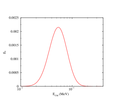
FIG. 1.: Sensitivity function of Ref. [16], showing the change in ⁶Li BBN yields resulting from small changes in the $d(\alpha,\gamma)^{6}{\rm Li}$ cross section over narrow energy bins at the specified energies.

We have carried out a calculation of the alpha-deuteron radiative capture cross section, treating it as a six-body problem. The remainder of this paper describes this calculation, and it is organized as follows: In Section II, we describe wave functions used to compute the $d(\alpha,\gamma)^{6}{\rm Li}$ cross section. In Section III, we describe the electromagnetic current operators and the methods used to calculate their matrix elements. In Section IV, we describe our results for the cross section, thermal reaction rates and nucleosynthesis yields, and in Section V, we summarize our results and discuss their implications.

II wave functions

A ${}^{2}{\rm H}$, ${}^{4}{\rm He}$, and ${}^{6}{\rm Li}$ ground states

The wave functions $|\psi_{d}^{m_{d}}\rangle$, $|\psi_{\alpha}\rangle$, and $|\psi_{{\rm Li}}^{m_{6}}\rangle$ used in our calculation are the ground states derived from the Argonne $v_{18}$ two-nucleon [17] and Urbana IX [18] three-nucleon potentials, henceforth denoted as the AV18/UIX model. The deuteron wave function is a direct numerical solution, while the variational Monte Carlo technique described in Refs. [19, 20, 21] is used to generate the ${}^{4}{\rm He}$ and ${}^{6}{\rm Li}$ wave functions. Here $m_{d}$ and $m_{6}$ denote spin orientation.

The variational trial functions for light nuclei are constructed from correlation operators acting on a Jastrow wave function:

$$|\Psi_{T}\rangle=\left[1+\sum_{i<j<k}\tilde{U}^{TNI}_{ijk}\right]\left[{\cal S}\prod_{i<j}(1+U_{ij})\right]|\Psi_{J}\rangle\ ,$$ (1)

where $U_{ij}$ and $\tilde{U}^{TNI}_{ijk}$ are two- and three-body correlation operators that include significant spin and isospin dependence and ${\cal S}$ is a symmetrization operator, needed because the $U_{ij}$ do not commute. For ${}^{4}{\rm He}$, the Jastrow part takes a relatively simple form:

$$|\Psi_{J}\rangle=\prod_{i<j<k\leq 4}f_{ijk}\prod_{i<j\leq 4}f(r_{ij})|\Phi_{\alpha}(0000)_{1234}\rangle\ ,$$ (2)

where $f(r_{ij})$ and $f_{ijk}$ are pair and triplet functions of relative position only, and $\Phi_{\alpha}(0000)$ is a determinant in the spin-isospin space of the four particles.

For ${}^{6}{\rm Li}$ the Jastrow part has a considerably more complicated structure due to the need to place the fifth and sixth particles in the p-shell:

$$|\Psi_{J}\rangle = {\cal A}\left\{\prod_{i<j<k\leq 4}f^{sss}_{ijk}\prod_{n\leq 4}f^{spp}_{n56}\prod_{i<j\leq 4}f_{ss}(r_{ij})\prod_{k\leq 4}f_{sp}(r_{k5})f_{sp}(r_{k6})\right.f_{pp}(r_{56})$$ (4)

$$\left.\sum_{LS}\Big{(}\beta_{LS}|\Phi_{6}(LSJMTT_{3})_{1234:56}\rangle\Big{)}\right\}\ .$$

The ${\cal A}$ is an antisymmetrization operator over all partitions of the six particles into groups of four plus two. The central pair and triplet correlations $f_{xy}(r_{ij})$ and $f^{xyz}_{ijk}$ have been generalized, with the $xyz$ denoting whether the particles are in the s- or p-shell. The wave function $|\Phi_{6}(LSJMTT_{3})\rangle$ has orbital angular momentum $L$ and spin $S$ coupled to total angular momentum $J$, projection $M$, isospin $T$, and charge state $T_{3}$, and is explicitly written as

$$|\Phi_{6}(LSJMTT_{3})_{1234:56}\rangle=|\Phi_{\alpha}(0000)_{1234}\phi^{LS}_{p}(R_{\alpha 5})\phi^{LS}_{p}(R_{\alpha 6})$$ (5)

$$\left\{[Y_{1m_{l}}(\Omega_{\alpha 5})Y_{1m_{l}^{\prime}}(\Omega_{\alpha 6})]_{LM_{L}}\times[\chi_{5}(\frac{1}{2}m_{s})\chi_{6}(\frac{1}{2}m_{s}^{\prime})]_{SM_{S}}\right\}_{JM}$$ (6)

$$\times[\nu_{5}(\frac{1}{2}t_{3})\nu_{6}(\frac{1}{2}t_{3}^{\prime})]_{TT_{3}}\rangle\ .$$ (7)

Particles 1–4 are placed in the s-shell core with only spin-isospin degrees of freedom, while particles 5–6 are placed in p-wave orbitals $\phi^{LS}_{p}(R_{\alpha k})$ that are functions of the distance between the center of mass of the core and the particle. Different amplitudes $\beta_{LS}$ are mixed to obtain an optimal wave function; for the $J^{\pi},T=1^{+},0$ ground state of ⁶Li the p-shell can have $\beta_{01}$, $\beta_{21}$, and $\beta_{10}$ terms.

The two-body correlation operator $U_{ij}$ is defined as:

$$U_{ij}=\sum_{p=2,6}\left[\prod_{k\not=i,j}f^{p}_{ijk}({\bf r}_{ik},{\bf r}_{jk})\right]u_{p}(r_{ij})O^{p}_{ij}\ ,$$ (8)

where the $O^{p=2,6}_{ij}$ = ${\mathchoice{{\hbox{\boldmath$\displaystyle\tau$}}}{{\hbox{\boldmath$\textstyle\tau$}}}{{\hbox{\boldmath$\scriptstyle\tau$}}}{{\hbox{\boldmath$\scriptscriptstyle\tau$}}}}_{i}\cdot{\mathchoice{{\hbox{\boldmath$\displaystyle\tau$}}}{{\hbox{\boldmath$\textstyle\tau$}}}{{\hbox{\boldmath$\scriptstyle\tau$}}}{{\hbox{\boldmath$\scriptscriptstyle\tau$}}}}_{j}$, ${\mathchoice{{\hbox{\boldmath$\displaystyle\sigma$}}}{{\hbox{\boldmath$\textstyle\sigma$}}}{{\hbox{\boldmath$\scriptstyle\sigma$}}}{{\hbox{\boldmath$\scriptscriptstyle\sigma$}}}}_{i}\cdot{\mathchoice{{\hbox{\boldmath$\displaystyle\sigma$}}}{{\hbox{\boldmath$\textstyle\sigma$}}}{{\hbox{\boldmath$\scriptstyle\sigma$}}}{{\hbox{\boldmath$\scriptscriptstyle\sigma$}}}}_{j}$, ${\mathchoice{{\hbox{\boldmath$\displaystyle\sigma$}}}{{\hbox{\boldmath$\textstyle\sigma$}}}{{\hbox{\boldmath$\scriptstyle\sigma$}}}{{\hbox{\boldmath$\scriptscriptstyle\sigma$}}}}_{i}\cdot{\mathchoice{{\hbox{\boldmath$\displaystyle\sigma$}}}{{\hbox{\boldmath$\textstyle\sigma$}}}{{\hbox{\boldmath$\scriptstyle\sigma$}}}{{\hbox{\boldmath$\scriptscriptstyle\sigma$}}}}_{j}{\mathchoice{{\hbox{\boldmath$\displaystyle\tau$}}}{{\hbox{\boldmath$\textstyle\tau$}}}{{\hbox{\boldmath$\scriptstyle\tau$}}}{{\hbox{\boldmath$\scriptscriptstyle\tau$}}}}_{i}\cdot{\mathchoice{{\hbox{\boldmath$\displaystyle\tau$}}}{{\hbox{\boldmath$\textstyle\tau$}}}{{\hbox{\boldmath$\scriptstyle\tau$}}}{{\hbox{\boldmath$\scriptscriptstyle\tau$}}}}_{j}$, $S_{ij}$, and $S_{ij}{\mathchoice{{\hbox{\boldmath$\displaystyle\tau$}}}{{\hbox{\boldmath$\textstyle\tau$}}}{{\hbox{\boldmath$\scriptstyle\tau$}}}{{\hbox{\boldmath$\scriptscriptstyle\tau$}}}}_{i}\cdot{\mathchoice{{\hbox{\boldmath$\displaystyle\tau$}}}{{\hbox{\boldmath$\textstyle\tau$}}}{{\hbox{\boldmath$\scriptstyle\tau$}}}{{\hbox{\boldmath$\scriptscriptstyle\tau$}}}}_{j}$, and the $f^{p}_{ijk}$ is an operator-independent three-body correlation. The six radial functions $f_{ss}(r)$ and $u_{p=2,6}(r)$ are obtained from two-body Euler-Lagrange equations with variational parameters as discussed in detail in Ref. [19]. Here we take them to be the same as in ${}^{4}{\rm He}$, except that the $u_{p=2,6}(r)$ are forced to go to zero at large distance by multiplying in a cutoff factor, $\Big{[}1+{\rm exp}[-R_{u}/a_{u}]\Big{]}/\Big{[}1+{\rm exp}[(r-R_{u})/a_{u}]\Big{]}$, with $R_{u}$ and $a_{u}$ as variational parameters. The $f_{sp}$ correlation is constructed to be similar to $f_{ss}$ for small separations, but goes to a constant of order unity at large distances:

$$f_{sp}(r)=\Bigg{[}a_{sp}+\frac{b_{sp}}{1+{\rm exp}[(r-R_{sp})/a_{sp}]}\Bigg{]}f_{ss}(r)+c_{sp}(1-\exp[-(r/d_{sp})^{2}])\ ,\\$$ (9)

where $a_{sp}$, $b_{sp}$, etc. are additional variational parameters. The $f_{pp}(r)$ correlation is given by:

$$f_{pp}(r)=u_{d}(r)/{[1-3u_{2}(r)+u_{3}(r)-3u_{4}(r)]r}\ ,$$ (10)

where $u_{d}(r)$ is the $S$-wave part of the exact deuteron wave function. Then $U_{ij}$ acting on the pair of nucleons in the p-shell will regenerate the correct deuteron $S$-wave and an effective $D$-wave $w_{d}(r)=f_{pp}(r)[u_{5}(r)-3u_{6}(r)]\sqrt{8}r$ from the tensor components. While the $D$-wave is not exact, we find that the resulting effective deuteron energy is $-2.16$ MeV, quite close to the correct value.

These choices for $f_{ss}$, $f_{sp}$, $f_{pp}$, and $u_{p=2,6}$ guarantee that when the two p-shell particles are far from the s-shell core, the overall wave function factorizes as:

$$\Psi_{T}\rightarrow[\phi^{LS}_{p}(R_{\alpha d})]^{2}\psi_{\alpha}\psi_{d}\ ,$$ (11)

where $\psi_{\alpha}$ is the variational ${}^{4}{\rm He}$ wave function and $\psi_{d}$ is (almost) the exact deuteron wave function.

The single-particle functions $\phi^{LS}_{p}(R_{\alpha n})$ describe correlations between the s-shell core and the p-shell nucleons, and have been taken in previous work [21] to be solutions of a radial Schrödinger equation for a Woods-Saxon potential and unit angular momentum, with energy and Woods-Saxon parameters determined variationally. It is important for low-energy radiative captures that these functions reproduce faithfully the large-separation behavior of the wave function, because the matrix elements receive large contributions at cluster separations greater than 10 fm. In fact, below 400 keV, more than 15% of the electric quadrupole operator comes from cluster separations beyond 30 fm. We have therefore modified the ${}^{6}{\rm Li}$ wave function for the capture calculation to enforce cluster-like behavior when the two p-shell nucleons are both far from the s-shell core.

In general, for light p-shell nuclei with an asymptotic two-cluster structure, such as $\alpha d$ in ${}^{6}{\rm Li}$ or $\alpha t$ in ⁷Li, we want the large separation behavior to be

$$[\phi^{LS}_{p}(r\rightarrow\infty)]^{n}\propto W_{km}(2\gamma r)/r,$$ (12)

where $W_{km}(2\gamma r)$ is the Whittaker function for bound-state wave functions in a Coulomb potential (see below) and $n$ is the number of p-shell nucleons. We achieve this by solving the equation

$$\Bigg{[}-\frac{\hbar^{2}}{2\mu_{41}}\Bigg{(}\frac{d^{2}}{dr^{2}}-\frac{\ell(\ell+1)}{r^{2}}\Bigg{)}+V(r)+\Lambda(r)\Bigg{]}r\phi^{LS}_{p}(r)=0,$$ (13)

with $\ell=1$, $\mu_{41}$ the reduced mass of one nucleon against four, and $V(r)$ a parametrized Woods-Saxon potential plus Coulomb term:

$$V(r)=\frac{V_{0}}{1+{\rm exp}[(r-R_{0})/a_{0}]}+\frac{2(Z-2)}{n}\frac{e^{2}}{r}F(r)\ .$$ (14)

Here $V_{0}$, $R_{0}$, and $a_{0}$ are variational parameters, $(Z-2)/n$ is the average charge of a p-shell nucleon, and F(r) is a form factor obtained by folding $\alpha$ and proton charge distributions together. The $\Lambda(r)$ is a Lagrange multiplier that enforces the asymptotic behavior at large $r$, but is cut off at small $r$ by means of a variational parameter $c_{0}$:

$$\Lambda(r)=\lambda(r)\Big{[}1-{\rm exp}\Big{(}-(r/c_{0})^{2}\Big{)}\Big{]}\ .$$ (15)

The $\lambda(r)$ is given by

$$\lambda(r)=\frac{\hbar^{2}}{2\mu_{41}}\Bigg{[}\frac{1}{u_{L}}\frac{d^{2}u_{L}}{dr^{2}}-\frac{2}{r^{2}}\Bigg{]}-\frac{2(Z-2)}{n}\frac{e^{2}}{r}\ ,$$ (16)

where $u_{L}$ is directly related to the Whittaker function:

$$u_{L}/r=(W_{km}(2\gamma r)/r)^{1/n}\ .$$ (17)

Here $\gamma^{2}=2\mu_{4n}B_{4n}/\hbar^{2}$, with $\mu_{4n}$ and $B_{4n}$ the appropriate two-cluster effective mass and binding energy, $k=-2(Z-2)e^{2}\mu_{4n}/\hbar^{2}\gamma$, and $m=L+\frac{1}{2}$.

For ${}^{6}{\rm Li}$, $B_{42}=1.47$ MeV and $L=0$, 2 corresponding to the asymptotic $S$- and $D$-waves of the ${}^{6}{\rm Li}$ ground state, or amplitudes $\beta_{01}$ and $\beta_{21}$ in Eq.(4). There is no asymptotic $\alpha d$ cluster corresponding to the $L=1$ amplitude $\beta_{10}$. Nevertheless, the energy of the ${}^{6}{\rm Li}$ ground state is variationally improved $\approx 0.1$ MeV by including such a component in the wave function, so we set the asymptotic behavior of $\phi^{10}_{p}(r)$ to a binding energy of 3.70 MeV, which is the threshold for ${}^{6}{\rm Li}\rightarrow\ ^{4}{\rm He}+p+n$ breakup.

In Refs. [20, 21] the $f^{sss}_{ijk}$ three-body correlation of Eq.(4) was a valuable and inexpensive improvement to the trial function, but no $f^{ssp}_{ijk}$ or $f^{spp}_{ijk}$ correlations could be found that were of any benefit. However, in the present work we find the correlation

$$f^{spp}_{n56}=1+q_{1}[f_{ss}(r_{56})/f_{pp}(r_{56})-1]{\rm exp}[-q_{2}(r_{n5}+r_{n6})]\ ,$$ (18)

with $q_{1,2}$ as variational parameters, to be very useful. It effectively alters the central pair correlation between the two p-shell nucleons from their asymptotic, deuteron-like form to be more like the pair correlations within the s-shell when the two particles are close to the core. This correlation improves the binding energy by $\approx 0.5$ MeV.

In Refs. [9, 21] we reported energies for the trial function $\Psi_{T}$ of Eq.(1), and for a more sophisticated variational wave function, $\Psi_{V}$, which adds two-body spin-orbit and three-body spin- and isospin-dependent correlation operators. The $\Psi_{V}$ gives improved binding compared to $\Psi_{T}$ in both ${}^{4}{\rm He}$ and ${}^{6}{\rm Li}$, but is significantly more expensive to construct because of the numerical derivatives required for the spin-orbit correlations. In the case of an energy calculation the derivatives are also needed for the evaluation of $L$-dependent terms in AV18, so the cost is only a factor of two in computation. However for the evaluation of other expectation values the relative cost increase is $\approx 6A$. Thus in the present work we choose to use $\Psi_{T}$ for non-energy evaluations; this proved quite adequate in our studies of ${}^{6}{\rm Li}$ form factors [10].

The variational Monte Carlo (VMC) energies and point proton rms radii obtained with $\Psi_{T}$ and $\Psi_{V}$ are shown in Table I along with the results of essentially exact Green’s function Monte Carlo (GFMC) calculations and the experimental values. We note that the underbinding of ${}^{6}{\rm Li}$ in the GFMC calculation is the fault of the AV18/UIX model and not the many-body method; it can be corrected by the introduction of more sophisticated three-nucleon potentials [22].

TABLE I.: Calculated VMC, GFMC, and experimental energies and point proton rms radii of ²H, ⁴He and ⁶Li. Numbers in parentheses are Monte Carlo statistical errors, or experimental uncertainties.

Nucleus	Observable	VMC		$GFMC$	$Experiment$
		$\Psi_{T}$	$\Psi_{V}$
2H	E	$--2.2246$			$--2.2246$
	$\langle r^{2}_{p}\rangle^{1/2}$	$1.967$			$1.953(3)$
4He	E	$--26.89(3)$	$--27.78(3)$	$--28.34(4)$	$--28.30$
	$\langle r^{2}_{p}\rangle^{1/2}$	$1.48(1)$	$1.47(1)$	$1.45(1)$	$1.48(1)$
6Li	E	$--27.19(5)$	$--28.21(4)$	$--31.15(11)$	$--31.99$
	$\langle r^{2}_{p}\rangle^{1/2}$	$2.46(2)$	$2.46(2)$	$2.57(1)$	$2.43(4)$

The present variational trial functions with the imposed proper asymptotic behavior in fact give slightly better energies than the older shell-model-like correlations of Refs. [9, 21]. Unfortunately, because the variational ${}^{6}{\rm Li}$ energy is not below that of separated alpha and deuteron clusters, it is possible to lower the energy significantly by making the wave function more and more diffuse. Therefore, the variational parameters were constrained to give a reasonable rms radius, as seen in Table I. Although the variational ${}^{6}{\rm Li}$ wave function remains unbound relative to alpha-deuteron breakup, it has the correct energy at large particle separations, as shown in Fig. 2. There we show the local energy, $E({\bf R})$, which is the energy for a given spatial configuration ${\bf R}=({\bf r}_{1},\dots,{\bf r}_{6})$, binned with its Monte Carlo statistical variance as a function of the sum $R=\sum_{i}|{\bf r}_{i}|$ of the particle distances from the center of mass. The average energy is shown by the solid line, while the dashed line gives the experimental binding. At the bottom of the figure is a histogram of the number of samples to show their distribution with $R$. We observe that the energy in compact configurations is clearly too small, but for $R>18$ fm the energies scatter about the experimental binding.

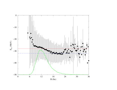
FIG. 2.: Monte Carlo local energy of the ${}^{6}{\rm Li}$ variational ground state binned as a function of the sum of the magnitudes of the particle coordinates, $R$. The horizontal solid line is the average variational energy and the horizontal dashed line indicates the experimental binding. The curve superimposed on the bottom is a histogram of the location of the 50 000 samples of $\Psi_{V}$ used in the calculation.

The asymptotic two-cluster behavior of our six-body wave function can be studied by computing the two-cluster $\alpha d$ distribution function, $\langle{\cal A}\psi_{\alpha}\psi_{d}^{m_{d}},{\bf r}_{\alpha d}\mid\psi_{\rm Li}^{m_{6}}\rangle$, described in Ref. [23]. It can be expressed in terms of Clebsch-Gordan factors, $Y_{LM}(\Omega_{\alpha d})$, and two radial functions $R_{L}(r_{\alpha d})$ for the $S$- and $D$-waves, which are plotted in Fig. 3. The $R_{L}$ can be used to extract the asymptotic normalization constants $C_{0}$ and $C_{2}$, by taking their ratio with the corresponding Whittaker functions, and the asymptotic $D/S$ ratio $\eta$. We find that $C_{0}$ does not become asymptotic until $r_{\alpha d}\gtrsim 8$ fm, where we obtain $C_{0}=2.28\pm 0.02$. However, $\eta$ is already asymptotic for $r_{\alpha d}\gtrsim 4$ fm, with the value $-0.026\pm 0.001$.

This value of $C_{0}$ is at the lower end of the range of values (2.3–2.9) used in a number of other studies [24, 25, 26]. However, the value of $\eta$ is consistent with the recent analysis of ${}^{6}{\rm Li}$ + ${}^{4}{\rm He}$ elastic scattering [26], which obtains $-0.025\pm 0.006\pm 0.010$. This is a big improvement over our earlier value of $-0.07\pm 0.02$ reported in Ref. [23], which was obtained with the shell-model-like wave function. However, our quadrupole moment $Q=-0.71\pm 0.08$ fm² remains an order of magnitude too large compared to the experimental value of $-0.08$ fm². The integrated $D^{\alpha d}_{2}$ parameter value is $-0.27\pm 0.01$ fm².

The spectroscopic factor is 0.86, in good agreement with the Robertson value of $0.85\pm 0.04$ [13]. The spectroscopic factor is not very sensitive to the asymptotic behavior of the wave function, and differs little from our earlier value of 0.84 obtained with the shell-model-like wave function. We note that our shell-model-like wave functions for ⁷Li and ⁶He provided an excellent prediction for the spectroscopic factors observed in ${}^{7}{\rm Li}(e,e^{\prime}p)$ scattering [27].

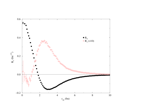
FIG. 3.: Monte Carlo samples of the radial two-cluster $\alpha d$ distribution functions in ${}^{6}{\rm Li}$.

B ${\bf\alpha}$d initial state

The initial alpha-deuteron scattering wave function $|\psi_{\alpha d};LSJM\rangle$ having orbital angular momentum $L$ and channel spin $S$ (=1) coupled to total $JM$, is expressed as

$$|\psi_{\alpha d};LSJM\rangle={\cal A}\left\{\phi_{\alpha d}(r_{\alpha d})Y_{LM_{L}}({\bf\hat{r}}_{\alpha d})\prod_{ij}G_{ij}|\psi_{\alpha}\psi_{d}^{m_{d}}\rangle\right\}_{LSJM},$$ (19)

where curly braces indicate angular momentum coupling, $\cal{A}$ antisymmetrizes between clusters, and ${\bf r}_{\alpha d}$ denotes the separation between the centers of mass of the $\alpha$ and $d$ clusters.

Our scattering wave function is built from the alpha and deuteron ground-state wave fuctions, $\psi_{\alpha}$ and $\psi_{d}^{m_{d}}$ (where $m_{d}$ denotes the deuteron spin projection), from a nucleon pair correlation operator $G_{ij}$, and from an intercluster scalar correlation $\phi_{\alpha d}(r_{\alpha d})$. $G_{ij}$ is the identity operator if particles $i$ and $j$ belong to the same cluster (alpha or deuteron). Otherwise, it is a pair correlation operator derived to describe nuclear matter [28], and it contains both central and non-central terms. It takes into account, in an approximate way, the distortions introduced in each cluster by the interactions with the particles in the other cluster, and becomes the identity operator as particle separations become large.

The intercluster correlation $\phi_{\alpha d}(r_{\alpha d})$ is a two-body radial wave function describing alpha-deuteron scattering as the scattering of two point particles. It is generated from a Schrödinger equation, with the potential chosen to reproduce the results of phase-shift analyses of alpha-deuteron scattering data in the two-body model. Several such potentials exist in the literature, and we saw no need to re-fit the data. The potentials which we have applied to this study are the potentials of Kukulin and Pomerantsev, Refs. [29, 30] (hereafter, “KP I” and “KP II”, respectively), and the potential of Langanke, Ref. [31]. Because the potential of Langanke was produced for the slightly different problem of describing the $\alpha d$ system in the resonating group method, it required modification to match our purposes. This consisted of a small adjustment to the Woods-Saxon radius to reproduce the energy of the $3^{+}$ resonance derived from electron scattering, 711 keV. The most important difference between these potentials, which give very similar cross sections in our calculations, is that the KP potentials were fitted to the phase shifts in the odd and even partial waves separately, to produce the expected parity-dependent potential. The work by Langanke was concerned only with even partial waves, and did not fit the odd partial waves, although it provides a fair qualitative description of the $P$-wave phase shifts at low energy.

The potentials are very similar to each other in form. All of the potentials used contain both central and spin-orbit terms, and the spin-orbit force in the even partial waves is well-constrained by the spacing of the $D$-wave scattering resonances. While a tensor component could in principle be derived to reproduce the ground-state quadrupole moment (assuming total alpha-deuteron cluster parentage of the ground state), its effect on the scattering data is too small to support deriving it from the scattering phase shifts. (A more ambitious approach to derive a tensor interaction would involve computing energies at fixed separation between the $\alpha$ and $d$ clusters and varying the deuteron orientation; however, we have not pursued such an approach here.) Coupling to other (e.g., cluster breakup) channels has also been neglected; this is well-justified below the ${}^{5}{\rm He}+p$ and ${}^{5}{\rm Li}+n$ thresholds at 3.12 and 4.20 MeV, respectively. We note that although the KP potentials and the Langanke potential all reproduce the scattering phase shifts very well, and they produce very similar ground-state wave functions at small cluster separation, the ground-state binding of the KP II potential is too large by almost a factor of two. All of the potentials we used to generate $\phi_{\alpha d}$ are deep potentials with a forbidden zero-node state. They produce the expected one-node structure of the ground-state alpha-deuteron wave function required by the Pauli principle, as illustrated by our $R_{L}$ functions in Fig.3, and enforce (by orthogonality to the forbidden state) the most important consequences of the Pauli principle for $\phi_{\alpha d}$.

A complication arises from the phenomenological treatment of the initial state. In reality, the ground-state and $S$-wave scattering-state wave functions are orthogonal, because they are different eigenstates of the same ($J^{\pi}=1^{+}$) potential. Because our calculation does not generate them explicitly as such, our ground state and $S$-wave scattering states are not necessarily orthogonal. For purposes of our capture calculation, this has the effect of generating spurious contributions to the $M1$ transition operator. For $S$-wave captures, we have modified the initial state to ensure orthogonality with the ground state. This is done by subtracting from the initial state, Eq.(19), its projection onto a complete set of ground states,

$$|\psi_{\alpha d};LSJM\rangle^{\prime}=|\psi_{\alpha d};LSJM\rangle-\sum_{m_{6}}|\psi_{\rm Li}^{m_{6}}\rangle\langle\psi_{\rm Li}^{m_{6}}|\psi_{\alpha d};LSJM\rangle\ ,$$ (20)

and computing $M1$ transitions from the adjusted state. This procedure reduced the $M1$ contribution to our computed cross sections by more than a factor of 10, roughly to the level of Monte Carlo sampling noise. Further evidence that the remaining contribution is spurious is its strong dependence on the phenomenological radial correlation in the scattering state, discussed below.

III Cross Section and Transition Operators

The cross section for $\alpha$$d$ radiative capture at c.m. energy $E_{c.m.}$ can be written as [32]

$$\sigma(E_{c.m.})=\frac{8\pi}{3}\frac{\alpha}{v_{\rm rel}}\frac{q}{1+q/m_{\rm Li}}\sum_{LSJ\ell}\Bigg{[}\left|E^{LSJ}_{\ell}(q)\right|^{2}+\left|M^{LSJ}_{\ell}(q)\right|^{2}\Bigg{]}\ ,$$ (21)

where $\alpha$ is the fine structure constant ($\alpha=e^{2}$; we take $\hbar=c=1$ in this Section), $v_{\rm rel}$ is the $\alpha$$d$ relative velocity, and $E^{LSJ}_{\ell}(q)$ and $M^{LSJ}_{\ell}(q)$ are the reduced matrix elements (RMEs) of the electric and magnetic multipole operators connecting the $\alpha$$d$ scattering state in channel $LSJ$ to the ⁶Li ground state having $J^{\pi},T=1^{+}$,0. The c.m. energy of the emitted photon is given by

$$q = m_{\rm Li}\Bigg{[}-1+\sqrt{1+\frac{2}{m_{\rm Li}}(m_{d}+m_{\alpha}-m_{\rm Li}+E_{c.m.})}\Bigg{]}$$ (22)

$$\simeq m_{d}+m_{\alpha}-m_{\rm Li}+E_{c.m.}\ ,$$ (23)

where $m_{d}$, $m_{\alpha}$, and $m_{\rm Li}$ are the rest masses of deuteron, ⁴He, and ⁶Li, respectively. The astrophysical $S$-factor is then related to the cross section via

$$S(E_{c.m.})=E_{c.m.}\,\sigma(E_{c.m.})\,{\rm exp}(4\,\pi\,\alpha/v_{\rm rel})\ .$$ (24)

The $M1$, $M2$, $E1$, $E2$, and $E3$ transitions involving $\alpha$$d$ scattering states with relative orbital angular momentum up to $L=2$ have been retained in the evaluation of the cross section. Initial states with $L=3$ and $L=4$ were examined in the early phases of this work, but proved to be very small, and were not retained in the final calculation.

Since the energies of interest in the present study are below 4 MeV, and consequently $qR_{\rm Li}\leq 0.05$ ($R_{\rm Li}$ is the ⁶Li point rms radius), the long-wavelength aproximation (LWA) of the multipole operators would naively be expected to be adequate to compute the associated RMEs. While the LWA is indeed sufficient for $E2$ transitions, which dominate the cross section at energies $E_{c.m.}>400$ keV, it is however inaccurate to compute the RMEs of $M1$ and, particularly, $E1$ transitions in the LWA since these are suppressed. (This fact has already been alluded to in the introduction). It is therefore necessary to include higher order terms, beyond the leading one which normally is taken to define the LWA, in the expansion in powers of $q$, so-called “retardation terms”. It is useful to review how these corrections arise for $E1$ transitions. We should point out that some of these same issues have recently been discussed in Ref. [33], in the context of a calculation of $E1$ strength in $d$$p$ radiative capture at energies below 100 keV.

A The $E_{1}$ operators

In principle, the $E1$ RMEs are obtained from

$$E_{1}^{LSJ}(q)={\sqrt{3}\over\langle JM,1\lambda|1m_{6}\rangle}\langle\Psi_{\rm Li}^{m_{6}}|E_{1\lambda}(q)|\psi_{\alpha d};LSJM\rangle\ ,$$ (25)

$$E_{1\lambda}(q)={1\over q}\int d{\bf x}\>{\bf j}({\bf x})\cdot\nabla\times j_{1}(qx){\bf Y}_{1\lambda}^{11}(\hat{\bf x})\ ,$$ (26)

where ${\bf j}({\bf x})$ is the nuclear current density operator, $j_{1}(qx)$ is the spherical Bessel function of order one, and ${\bf Y}_{1\lambda}^{11}(\hat{\bf x})$ are vector spherical harmonic functions. For ease of presentation, the factor $\sqrt{3}/\langle JM,1\lambda|1m_{6}\rangle$ occurring in the definition of the RMEs will be suppressed in the following discussion. By expanding the Bessel function in powers of $q$ and after standard manipulations [34], the $E_{1}$ operator can be expressed as

$$E_{1\lambda}(q)\simeq E_{1\lambda}(q;{\rm LWA1})+E_{1\lambda}(q;{\rm LWA2})+E_{1\lambda}(q;{\rm LWA3})\>\>\>,$$ (27)

where

$$E_{1\lambda}(q;{\rm LWA1})=-{\sqrt{2}\over 3}\left[H\,,\,\int d{\bf x}\>x\,Y_{1\lambda}(\hat{\bf x})\>\rho({\bf x})\right]\>\>\>,$$ (28)

$$E_{1\lambda}(q;{\rm LWA2})={{\rm i}\,q^{2}\over 3\sqrt{2}}\int d{\bf x}\,x\,Y_{1\lambda}(\hat{\bf x})\,{\bf x}\cdot{\bf j}({\bf x})\>\>\>,$$ (29)

$$E_{1\lambda}(q;{\rm LWA3})={\sqrt{2}\,q^{2}\over 15}\left[H\,,\,\int d{\bf x}\>x^{3}\,Y_{1\lambda}(\hat{\bf x})\>\rho({\bf x})\right]\>\>\>.$$ (30)

Here the continuity equation has been used to relate $\nabla\cdot{\bf j}({\bf x})$ occurring in $E_{1\lambda}(q;{\rm LWA1})$ and $E_{1\lambda}(q;{\rm LWA3})$ to the commutator $-{\rm i}[H\,,\,\rho({\bf x})]$, where $\rho({\bf x})$ is the charge density operator. Evaluating the RMEs of these operators leads to

$$E_{1}^{LSJ}(q)\simeq E_{1}^{LSJ}(q;{\rm LWA1})+E_{1}^{LSJ}(q;{\rm LWA2})+E_{1}^{LSJ}(q;{\rm LWA3})\ ,$$ (31)

with

$$E_{1}^{LSJ}(q;{\rm LWA1})={\sqrt{2}\,q\over 3}\langle\Psi_{\rm Li}^{m_{6}}|\int d{\bf x}\,xY_{1\lambda}(\hat{\bf x})\rho({\bf x})|\psi_{\alpha d};LSJM\rangle\ ,$$ (32)

$$E_{1}^{LSJ}(q;{\rm LWA2})={{\rm i}\,q^{2}\over 3\sqrt{2}}\langle\Psi_{\rm Li}^{m_{6}}|\int d{\bf x}\,xY_{1\lambda}(\hat{\bf x}){\bf x}\cdot{\bf j}({\bf x})|\psi_{\alpha d};LSJM\rangle\ ,$$ (33)

$$E_{1}^{LSJ}(q;{\rm LWA3})=-{\sqrt{2}\,q^{3}\over 15}\langle\Psi_{\rm Li}^{m_{6}}|\int d{\bf x}\,x^{3}Y_{1\lambda}(\hat{\bf x})\rho({\bf x})|\psi_{\alpha d};LSJM\rangle\ ,$$ (34)

where terms up to order $q^{3}$ have been retained, and it has been assumed that the initial and final VMC wave functions are exact eigenfunctions of the Hamiltonian – which, incidentally, is clearly not the case, see the previous Section – so that $[H\,,\,\rho({\bf x})]\rightarrow-q\,\rho({\bf x})$ in the matrix element, ignoring the kinetic energy of the recoiling ⁶Li.

The nuclear electromagnetic charge and current density operators have one- and two-body components.

$$\rho({\bf x}) = \sum_{i}\rho^{(1)}_{i}({\bf x})+\sum_{i<j}\rho^{(2)}_{ij}({\bf x})\>\>;$$ (35)

$${\bf j}({\bf x}) = \sum_{i}{\bf j}^{(1)}_{i}({\bf x})+\sum_{i<j}{\bf j}^{(2)}_{ij}({\bf x})\>\>.$$ (36)

The one-body terms $\rho^{(1)}_{i}$ and ${\bf j}^{(1)}_{i}$ have the standard expressions [34] obtained from a non-relativistic reduction of the covariant single-nucleon current. The charge density is written as

$$\rho^{(1)}_{i}({\bf x})=\rho^{(1)}_{i,{\rm NR}}({\bf x})+\rho^{(1)}_{i,{\rm RC}}({\bf x})\>\>,$$ (37)

with

$$\rho^{(1)}_{i,{\rm NR}}({\bf x})=\epsilon_{i}\>\delta({\bf x}-{\bf r}_{i})\>\>,$$ (38)

$$\rho^{(1)}_{i,{\rm RC}}({\bf x})={\frac{1}{8m^{2}}}\left(2\,\mu_{i}-\epsilon_{i}\right)\nabla_{x}\cdot\Bigg{[}\mathchoice{{\hbox{\boldmath$\displaystyle\sigma$}}}{{\hbox{\boldmath$\textstyle\sigma$}}}{{\hbox{\boldmath$\scriptstyle\sigma$}}}{{\hbox{\boldmath$\scriptscriptstyle\sigma$}}}_{i}\times{\bf p}_{i}\,,\,\delta({\bf x}-{\bf r}_{i})\Bigg{]}_{+}\>\>,$$ (39)

where the Darwin-Foldy relativistic correction has been neglected in the expression for $\rho^{(1)}_{i,{\rm RC}}$, since it gives no contribution to Eq. (32) (see below). Hereafter, $[\cdots\,,\,\cdots]_{+}$ denotes the anticommutator. The one-body current density is expressed as

$${\bf j}^{(1)}_{i}({\bf x})={\frac{1}{2m}}\epsilon_{i}\>\Biggl{[}{\bf p}_{i}\>,\>\delta({\bf x}-{\bf r}_{i})\Biggr{]}_{+}-{\frac{1}{2m}}\mu_{i}\>\mathchoice{{\hbox{\boldmath$\displaystyle\sigma$}}}{{\hbox{\boldmath$\textstyle\sigma$}}}{{\hbox{\boldmath$\scriptstyle\sigma$}}}{{\hbox{\boldmath$\scriptscriptstyle\sigma$}}}_{i}\times\nabla_{x}\delta({\bf x}-{\bf r}_{i})\ .$$ (40)

The following definitions have been introduced:

$$\epsilon_{i} \equiv \frac{1+\tau_{i,z}}{2}\>\>,$$ (41)

$$\mu_{i} \equiv \frac{\mu^{S}+\mu^{V}\tau_{i,z}}{2}\>\>,$$ (42)

where $\mu^{S}$ ($\mu^{S}$=0.88 n.m.) and $\mu^{V}$ ($\mu^{V}$=4.706 n.m.) are the isoscalar and isovector combinations of the proton and neutron magnetic moments.

The two-body charge and current density operators have pion range terms and additional, short-range terms due to heavy meson exchanges [32]. However, the pion-exchange current density is an isovector operator, and its matrix element vanishes identically in the radiative $\alpha$$d$ capture, while the heavy-meson exchange (charge and current) operators are expected to give negligible contributions. Hence, in the present study we only retain the charge density operator associated with pion exchange. It is explicitly given by

$$\rho^{(2)}_{ij,\pi}({\bf x})=-\frac{f^{2}_{\pi}}{2\,m\,m_{\pi}^{2}}\mathchoice{{\hbox{\boldmath$\displaystyle\tau$}}}{{\hbox{\boldmath$\textstyle\tau$}}}{{\hbox{\boldmath$\scriptstyle\tau$}}}{{\hbox{\boldmath$\scriptscriptstyle\tau$}}}_{i}\cdot\mathchoice{{\hbox{\boldmath$\displaystyle\tau$}}}{{\hbox{\boldmath$\textstyle\tau$}}}{{\hbox{\boldmath$\scriptstyle\tau$}}}{{\hbox{\boldmath$\scriptscriptstyle\tau$}}}_{j}\,I_{\pi}^{\prime}(r_{ij})\,\Bigg{[}\mathchoice{{\hbox{\boldmath$\displaystyle\sigma$}}}{{\hbox{\boldmath$\textstyle\sigma$}}}{{\hbox{\boldmath$\scriptstyle\sigma$}}}{{\hbox{\boldmath$\scriptscriptstyle\sigma$}}}_{j}\cdot\hat{\bf r}_{ij}\mathchoice{{\hbox{\boldmath$\displaystyle\sigma$}}}{{\hbox{\boldmath$\textstyle\sigma$}}}{{\hbox{\boldmath$\scriptstyle\sigma$}}}{{\hbox{\boldmath$\scriptscriptstyle\sigma$}}}_{i}\cdot\nabla_{x}\,\delta({\bf x}-{\bf r}_{i})\,+i\rightleftharpoons j\Bigg{]}\ ,$$ (43)

where $m_{\pi}$ is the charged pion mass, $f_{\pi}$ the pion-nucleon coupling constant ($f_{\pi}^{2}/4\pi=0.075$), ${\bf r}_{ij}={\bf r}_{i}-{\bf r}_{j}$ is the separation of nucleons $i$ and $j$, and the function $I_{\pi}(r)$ is defined as

$$I_{\pi}(r)=\frac{1}{4\pi r}\left[{\rm e}^{-m_{\pi}r}-{\rm e}^{-\Lambda_{\pi}r}-\frac{1}{2}\left(1-\frac{m_{\pi}^{2}}{\Lambda_{\pi}^{2}}\right)\Lambda_{\pi}r{\rm e}^{-\Lambda_{\pi}r}\right]\ .$$ (44)

The prime denotes differentiation with respect to its argument. For the parameter $\Lambda_{\pi}$, we have taken the value 1.05 GeV.

We now consider, in turn, the various contributions LWA1, LWA2, and LWA3 to the $E_{1}$ RME. Insertion of the NR, RC, and $\pi$-exchange charge density operators in Eq. (32) allows us to write correspondingly

$$E_{1}^{LSJ}(q;{\rm LWA1})\simeq E_{1}^{LSJ}(q;{\rm LWAc})+E_{1}^{LSJ}(q;{\rm LWAb})+E_{1}^{LSJ}(q;{\rm LWA}\pi)$$ (45)

where

$$E_{1}^{LSJ}(q;{\rm LWAc})={\sqrt{2}\,q\over 3}\langle\Psi_{\rm Li}^{m_{6}}|\sum_{i}\epsilon_{i}\,r_{i}\,Y_{1\lambda}(\hat{\bf r}_{i})|\psi_{\alpha d};LSJM\rangle\ ,$$ (46)

$$E_{1}^{LSJ}(q;{\rm LWAb})={\sqrt{2}\,q\over 3}\sqrt{\frac{3}{4\pi}}\langle\Psi_{\rm Li}^{m_{6}}|\sum_{i}-{2\mu_{i}-\epsilon_{i}\over 4m^{2}}(\mathchoice{{\hbox{\boldmath$\displaystyle\sigma$}}}{{\hbox{\boldmath$\textstyle\sigma$}}}{{\hbox{\boldmath$\scriptstyle\sigma$}}}{{\hbox{\boldmath$\scriptscriptstyle\sigma$}}}_{i}\times{\bf p}_{i})_{\lambda}|\psi_{\alpha d};LSJM\rangle\ ,$$ (47)

$$E_{1}^{LSJ}(q;{\rm LWA}\pi)={\sqrt{2}\,q\over 3}\sqrt{\frac{3}{4\pi}}\langle\Psi_{\rm Li}^{m_{6}}|\sum_{i<j} \frac{f_{\pi}^{2}}{2\,m\,m_{\pi}^{2}}\mathchoice{{\hbox{\boldmath$\displaystyle\tau$}}}{{\hbox{\boldmath$\textstyle\tau$}}}{{\hbox{\boldmath$\scriptstyle\tau$}}}{{\hbox{\boldmath$\scriptscriptstyle\tau$}}}_{i}\cdot\mathchoice{{\hbox{\boldmath$\displaystyle\tau$}}}{{\hbox{\boldmath$\textstyle\tau$}}}{{\hbox{\boldmath$\scriptstyle\tau$}}}{{\hbox{\boldmath$\scriptscriptstyle\tau$}}}_{j}\,I_{\pi}^{\prime}(r_{ij})\,\Bigg{[}\sigma_{i,\lambda}\,\mathchoice{{\hbox{\boldmath$\displaystyle\sigma$}}}{{\hbox{\boldmath$\textstyle\sigma$}}}{{\hbox{\boldmath$\scriptstyle\sigma$}}}{{\hbox{\boldmath$\scriptscriptstyle\sigma$}}}_{j}\cdot\hat{\bf r}_{ij}$$ (49)

$$+i\rightleftharpoons j\Biggr{]}|\psi_{\alpha d};LSJM\rangle\ ,$$

where $(\sigma\times{\bf p})_{\lambda}$ and $\sigma_{i,\lambda}$ denote spherical components.

Next, for the terms of order $q^{2}$ and $q^{3}$, Eqs. (33) and (34), we find:

$$E_{1}^{LSJ}(q;{\rm LWA2})={{\rm i}\,q^{2}\over 3\sqrt{2}}\langle\Psi_{\rm Li}^{m_{6}}|\sum_{i} \frac{\epsilon_{i}}{2\,m}\Bigg{[}{\bf p}_{i}\cdot\,,\,{\bf r}_{i}\,r_{i}\,Y_{1\lambda}(\hat{\bf r}_{i})\Bigg{]}_{+}$$ (50)

$$- \frac{\mu_{i}}{2\,m}\sqrt{\frac{3}{4\pi}}({\bf r}_{i}\times\mathchoice{{\hbox{\boldmath$\displaystyle\sigma$}}}{{\hbox{\boldmath$\textstyle\sigma$}}}{{\hbox{\boldmath$\scriptstyle\sigma$}}}{{\hbox{\boldmath$\scriptscriptstyle\sigma$}}}_{i})_{\lambda}|\psi_{\alpha d};LSJM\rangle\ ,$$ (51)

$$E_{1}^{LSJ}(q;{\rm LWA3})=-{\sqrt{2}\,q^{3}\over 15}\langle\Psi_{\rm Li}^{m_{6}}|\sum_{i}\epsilon_{i}\,r_{i}^{3}\,Y_{1\lambda}(\hat{\bf r}_{i})|\psi_{\alpha d};LSJM\rangle\ ,$$ (52)

where in the last equation the contributions from relativistic corrections and pion-exchange have been neglected.

The leading contribution $E_{1}^{LSJ}(q;{\rm LWAc})$ to the $E_{1}$ RME vanishes in $\alpha$$d$ capture, since the initial and final states have zero isospin, and the corresponding wave functions do not depend on the c.m. position:

$$E_{1}^{LSJ}({\rm LWAc})\propto\langle\Psi_{\rm Li}^{m_{6}}|\sum_{i}{\bf r}_{i,\lambda}|\psi_{\alpha d};LSJM\rangle=0\ ,$$ (53)

where the coordinates ${\bf r}_{i}$ are defined relative to that of the c.m..

There are also more subtle corrections, which can potentially lead to additional, (relatively) significant $E_{1}$ contributions. One such correction is the possibility of isospin admixtures with $T>0$ in the ⁶Li and $\alpha$$d$ states, originating from the isospin-symmetry-breaking interactions present in the AV18/UIX model. These $T>0$ components are ignored in the VMC wave functions used here.

An additional correction – which we take into account – arises from a relativistic correction to the center of mass, and makes the LWAc contribution nonzero. This correction arises because translation-invariant wave functions require not center-of-mass but center-of-energy coordinates. Such coordinates constitute the relativistic analog of the center-of-mass coordinates appropriate to nonrelativistic problems. The distinction is usually not crucial at low energies, but it matters here because the LWAc term would otherwise be zero. Since the coordinates in which we compute wave functions are not center-of-energy coordinates, the dipole moment

$${\bf d}=\sum_{i}\epsilon_{i}{\bf r}_{i},$$ (54)

which enters Eq. (53), should be replaced by the expression

$${\bf d} = \sum_{i}\epsilon_{i}({\bf r}_{i}-{\bf r}_{CE})$$ (55)

$$= -\sum_{i}\epsilon_{i}{\bf r}_{CE}\ ,$$ (56)

where

$${\bf r}_{CE}=\frac{\sum_{i}E_{i}{\bf r}_{i}}{\sum_{i}E_{i}}\ ,$$ (57)

and

$$E_{i}=m+\frac{p_{i}^{2}}{2m}+\frac{1}{2}\sum_{j\neq i}v_{ij}+\frac{1}{3}\sum_{j\neq k\neq i}V_{ijk}\ .$$ (58)

Here, $v_{ij}$ and $V_{ijk}$ are the two- and three-nucleon potentials. We have thus replaced the particle masses in the expression for center of mass by their total energies (rest energy plus kinetic and potential energies). Since the nucleon masses contribute most of the nucleons’ relativistic energies, the center of mass is only slightly different from the center of energy. (The rms radius of the center of energy for our ⁶Li variational ground state is $(9.1\pm 2.7)\times 10^{-3}$ fm.) We note that this correction has been taken into account in the past (in two-body models) by putting the measured alpha and deuteron masses into calculations, rather than $4m$ and $2m$ [13, 24, 25, 35, 36]. These differ by the mass defects of the alpha particle and deuteron.

The $E1$ cross sections arising from the center-of-energy correction are larger than the $E1$ cross sections measured in Ref. [13] by about a factor of six. There is a significant ($\simeq 30\%$) LWAb spin-orbit contribution which becomes more important with increasing energy; the next-largest contributions are from the LWA3 and LWA2 operators. All of these terms except LWAb are too small in our calculation to account for the observed transition by more than a factor of ten, but LWA3 is responsible for about 20% of the total $S$ factor at zero energy. We have also included the contribution labelled LWA$\pi$ in the present study, and we find it to be much smaller than LWAb. Note that although the LWAb term is large enough to account for the magnitude of the $E1$ data alone, it is of the wrong sign to account for the asymmetry from which the $E1$ strength is extracted.

B The Monte Carlo Calculation

We calculated matrix elements by modifying the variational Monte Carlo code described in Ref. [21] to perform Monte Carlo integrations of matrix elements between the scattering and ground states described above. The Monte Carlo algorithm used was the Metropolis algorithm, and we tried several weighting functions, all based on the ${}^{6}{\rm Li}$ ground state. The final calculation used the weighting function

$$W({\bf R})=\sqrt{\langle\psi_{\rm Li}^{m_{6}}({\bf R})|\psi_{\rm Li}^{m_{6}}({\bf R})\rangle}$$ (59)

(where the bra-ket product here indicates summation over spin and isospin degrees of freedom for a given spatial configuration ${\bf R}=({\bf r}_{1},{\bf r}_{2},\ldots,{\bf r}_{6})$ of the particles; in all other cases, it also indicates integration over space coordinates). This weighting function was chosen to reflect approximately the expected behavior of the matrix element, and to obtain good sampling both at small cluster separation and out to 40 fm cluster separation. In the low-energy calculation, 3% of the $E1$ matrix element and 15% of the $E2$ matrix element come from the region beyond 30 fm cluster separation.

Because all of the energy dependence is contained in the relative wave function $\phi_{\alpha d}(r_{\alpha d})$ and the transition operators, the matrix element for a given scattering partial wave can be re-written as

$$T^{LSJ}_{\ell}(q)=\int_{0}^{\infty}dx\,x^{2}\,\phi_{\alpha d}(x)\langle\psi_{\rm Li}^{m_{6}}|T_{\ell\lambda}(q){\cal A}\left\{\delta(x-r_{\alpha d})Y_{L}^{M_{L}}({\bf\hat{r}}_{\alpha d}))\prod_{ij}G_{ij}|\psi_{\alpha}\psi_{d}^{m_{d}}\rangle\right\}_{LSJM},$$ (60)

using a technique from Ref. [37]. Here $T_{\ell\lambda}$ denotes any of the $E_{\ell}$ and $M_{\ell}$ operators. The partial-wave expansion of the current operator contains the photon energy only in multiplicative factors on each term of the expansion. The integration over all coordinates except $x$ can therefore be calculated once for each partial wave by the Monte Carlo code, and the result can then be used to compute the full integral for as many energies as desired by recomputing $\phi_{\alpha d}$ only, greatly reducing the amount of computation.

The calculation sampled 2 000 000 Monte Carlo configurations, summing over all 15 partitions of the six particles into clusters at each step. Typical results for the integrand in Eq.(60) at low energy are shown for two transitions, at two different energies, in Fig. 4. Calculations at energies above about 1 MeV had integrands that were essentially zero beyond 30 fm cluster separation, and therefore suffered little from limited sampling.

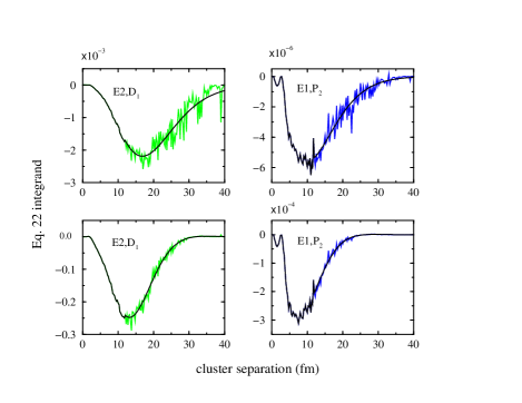
FIG. 4.: Upper panel: The integrand of Eq.(60) for $E2$ transitions from the $D_{1}$ initial state and $E1$ transitions from the $P_{2}$ initial state. The upper panels are for $E_{c.m.}=50$ keV, while the lower panels are for $E_{c.m.}=1$ MeV. “Noisy” curves are computed solely from the Monte Carlo integration (and their scatter indicates sampling uncertainty), while smooth curves show the expected long-range behavior of the operators, with normalization fitted to the Monte Carlo results.

We also performed a second set of calculations, this time computing functions which had the expected asymptotic forms of the operator densities as a function of $x$ at large cluster separations, and normalizing them to the Monte-Carlo sampled operator densities between 12 and 22 fm. These asymptotic forms, given by multiplying Eq. (12) by powers of $r_{\alpha d}$ appropriate for each operator, were then used instead of the Monte Carlo operator densities at cluster separations greater than 12 fm, in order to check that our results were not affected by the effective cutoff in sampling beyond 45 fm (due to very small $W({\bf R})$) or by poor sampling elsewhere in the tails of the wave function. For all of the dominant reaction mechanisms, this gave essentially the same result as the explicit calculation. The smooth curves of Fig. 4 were computed in this way.

IV Results

FIG. 5.: The total $S$-factor calculated from the Langanke (solid curve) and KP II potentials (dashed curve), with the data of [13] ($\triangle$), [14] ($\times$), and [15] ($\circ$). The indirect data of Ref. [15] were taken from their graphical presentation in [38].

Our main result is the total capture cross section as a function of energy, shown in comparison with laboratory data in Fig. 5 as an astrophysical $S$-factor. Note the good agreement with the capture data below 3 MeV, reflecting a reasonable value of the alpha-deuteron asymptotic normalization coefficient of the ⁶Li ground state, $C_{0}$, and accurate reproduction of the scattering phase shifts. The disagreement with the data above 3 MeV is a generic feature of direct-capture models, and is usually attributed to neglected couplings to breakup channels, and to channels with nonzero isospin in the scattering state (such as the $J^{\pi},T=0^{+},1$ state at 2.09 MeV). As shown in Fig. 6, the behavior at the $3^{+}$ resonance is nicely reproduced in location, width, and amplitude, simply by constraining the cluster potentials in the $D$ waves to reproduce the experimental phase shifts. The failure to match the energy dependence of the cross sections inferred below 500 keV from Coulomb-breakup experiments is shared by all other direct capture calculations, and could reflect either something that is not understood about the experiments, or something that is missing from the models. Our result with more detailed wave functions and operators than previously considered may be taken as a further indication that previous models were correct in this region.

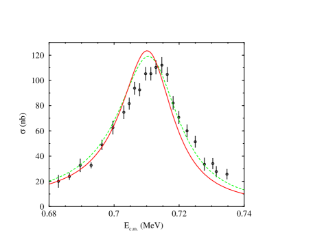
FIG. 6.: The calculated total cross section at the 711 keV resonance, compared with the data of Ref. [14]. The solid curve was computed from the Langanke potential, while the dashed curve was computed from the KP II potential.

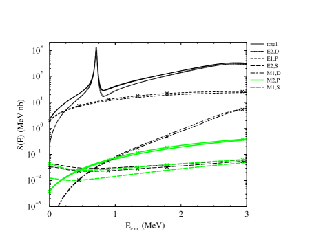
FIG. 7.: Contributions of the more important reaction multipolarities and incoming partial waves to the $S$ factor. Curves marked with the symbols $\times$ were computed from the Langanke effective potential; plain curves were computed from the KP II potential. Curve labels refer to reaction multipolarity and orbital angular momentum of the initial state.

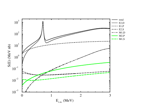
FIG. 8.: Contributions of reaction mechanisms and incoming partial waves to the $S$ factor, computed from the KP II potential. Cross sections were computed both using the plain Monte Carlo calculation, and normalizing the expected asymptotic form to the Monte Carlo operator densities; there are therefore two curves of each type, although they are indistinguishable for the total and for some of the mechanisms. Curve labels are as in Fig. 7.

In Figs. 7 and 8, we show the breakdown of the cross section into contributions from different multipolarities and incoming partial waves, again as $S$ factors. Fig. 7 shows results of two calculations, one from the Langanke potential and one from the KP II potential. The results are dominated by $E2$ transitions arising from $D$-wave scattering and by $E1$ transitions arising from $P$-wave scattering. Results from the two sets of scattering states are almost indistinguishable for these transitions, especially at low energies. In Fig. 8, the two sets of curves were both computed from the KP II potential. One set of curves was computed directly from the Monte Carlo calculation, while the other was computed from the expected asymptotic behavior of the integrand of Eq. 60 beyond 12 fm, as described above. Fig. 9 shows a further breakdown of the $E1$ operator into its various terms, along with the measured $E1$ contributions [13]. It is seen that:

1.) The $E1$ cross section is larger than the data of Robertson et al. [13] by a factor of about 7 at 2 MeV. Most other models have also arrived at $E1$ cross sections that are too large relative to these data. A new aspect of our calculation is that the largest contribution is calculated from the nucleon-nucleon potentials as a relativistic center-of-mass correction. This corresponds closely to inserting measured cluster masses by hand in simpler models, as indicated by the fact that virtually identical (within 50%) results for the LWAc term are obtained from our six-body model and from a simple capture model using the same cluster potential, but with laboratory alpha and deuteron masses introduced. In Fig. 9, the top curve is the total $E1$ $S$ factor (arising mainly from the center-of-energy correction), and the other curves indicate the $S$ factors that would result from various small terms in the E1 operator individually. (These differ from their actual contributions to the $S$ factor, since these contributions add coherently in the matrix element.) The center-of-energy and LWAb terms are obviously much more important than the other terms in our calculation, and the smaller terms do not affect the total significantly.

We note also that Robertson et al. [13] report the opposite sign from what is expected for the $E1$ transition in their experiment. None of the effects in our calculation can produce an effect of the correct magnitude with the observed “wrong” sign, or reproduce the sharp drop in $E1$ amplitude from 1.63 to 1.33 MeV seen in the data.

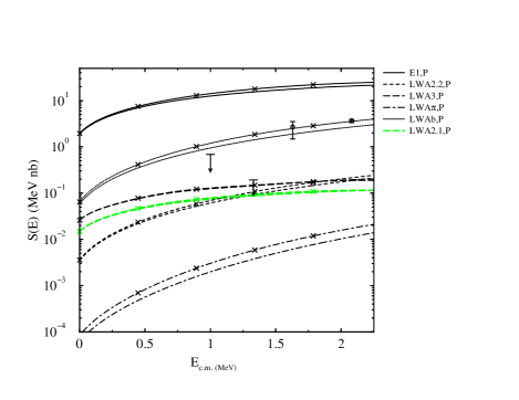
FIG. 9.: The total $E1$ operator (solid curves) and the cross sections resulting from each of the smaller terms of the operator acting individually, shown as $S$ factors. Plain curves were computed from the KP II potential. Curves with symbols $\times$ were computed from the Langanke potential. Labels for multipole and orbital angular momentum are as in Fig. 7. Other labels are as in Eqs. (45–52), except that LWA2.1 and LWA2.2 denote the first and second terms of Eq. 50, respectively. The data shown are the $E1$ cross sections and upper limits from Ref. [13].

2.) There is no significant $M1$ transition originating from the $S$-wave scattering state at lowest order in LWA, and we estimate the next-to-lowest term to be much smaller than what we obtain for the lowest-order term. The $M1$ strength is expected to be generally very small, since it is zero by orthogonality arguments in a two-body model. However, at very low energy, any $S$-wave contribution present may be expected to dominate the total cross section, and many-body wave functions can (in principle) provide small pieces of the final-state wave function which can be reached in such a transition. Such an effect is present in neutron captures on the deuteron and on ³He. The presence of a nonzero $M1$ contribution in our calculation raises two questions: to what extent is it a product of our choice of wave functions, and how will the presence of meson exchange currents (MEC), which is a factor-of-ten correction for the $M1$ cross section in ${}^{3}{\rm He}(n,\gamma)^{4}{\rm He}$, affect our result? The answer to the first question lies in the discussion of orthogonalization at the end of Sec. II and in Fig. 7; orthogonal ground and scattering states produce much smaller $M1$ contributions than non-orthogonalized states, and the remaining $M1$ contribution is very sensitive to the choice of phenomenological scattering potentials, suggesting a near-cancellation that ought to be exact. The second question is less important than it may appear at first glance. The large relative MEC contributions to neutron captures on light nuclei typically arise from the isovector part of the $M1$ operator. The $\alpha d$ capture process is isoscalar; the isoscalar MEC operator is both significantly smaller than the corresponding isovector operator, and quantitatively less certain in magnitude. We have therefore neglected MEC contributions to the M1 operator. Only electric multipoles contribute to Coulomb breakup, so the discrepancy between our results and the indirect data (circles in Fig. 5) is not the result of omitting MEC.

To compare our results with those obtained in a simpler model, we have also computed $\alpha d$ capture by treating the two clusters as point particles, and the ground state as an $S$-wave bound state of these two clusters. We used the modified Langanke potential, described above, to compute both states. With this potential, the ${}^{6}{\rm Li}$ ground state energy is 0.07 MeV too high, and this affects the energy dependence of the cross section. The asymptotic normalization of the wave function, which sets the scale for the nonresonant cross section, depends in any model on the detailed short-range behavior of the ground state, and is larger for this model than for our six-body ${}^{6}{\rm Li}$ ground state. While the 711 keV resonance is equally well-reproduced in strength and width by both two-body and six-body models, the total cross sections away from resonance are as much as 16% smaller in the six-body model. The simple model also yields an $E1$ strength which is greater by about 30% at 3 MeV. The source of the greater $E1$ strength is an interplay between the differing asymptotic normalizations, the treatment of the center-of-energy correction (treated in the simple model by using laboratory values of alpha and deuteron masses), and differences in the sizes of LWA2 and LWAb terms.

FIG. 10.: Thermally-averaged reaction rates, for the Langanke (solid) and KP II (dashed) potentials. The upper panel shows rates scaled to the temperature dependence expected for a constant $S$ factor (to make small differences visible), while the lower panel shows ratios to the rate of Robertson et al. [13]. Shown for comparison are the Robertson et al. rate (long-dashed), and the rate presently recommended in the NACRE compilation of reaction rates (dash-dotted) [38]. The line at the top indicates the approximate temperature range for big-bang production of ${}^{6}{\rm Li}$.

We have also calculated thermally-averaged reaction rates suitable for use in astrophysical calculations. We integrate from 0.1 keV to 10 MeV at temperatures from $10^{7}$ K to $3\times 10^{10}$ K to produce the quantity $N_{A}\langle\sigma v\rangle$ customarily used in reaction network calculations. Our result, shown in Fig. 10, is as much as 40% larger than previous estimates over a wide range of temperatures. The sources of these differences are not clear. They probably arise from several specific details of the capture models used, which have been normalized to the data using assumptions about the relative roles of the $E1$ and $E2$ components to produce the rates recommended in compilations.

V Discussion

The total cross sections we have computed compare favorably with the data in the region from the $3^{+}$ resonance to 3 MeV. This reflects mainly a combination of reasonable fits of the scattering states to experimental phase shifts, and reasonable reproduction of the asymptotic behavior of the ⁶Li ground state in the $S$-wave $\alpha d$ channel. Our calculation of the $E1$ cross section from the relativistic center-of-energy correction, and examination of several smaller corrections, is new; however, like all other models not actually scaled to the laboratory data, it is higher than the data. In our calculation, the $E1$ transition contributes just under 70% of the total cross section at 50 keV.

A very large cross section for alpha-deuteron capture would be of some interest for cosmology, since it would allow significant production of ${}^{6}{\rm Li}$ in the big bang. However, we find that big-bang nucleosynthesis calculations using our new cross sections can produce ${}^{6}{\rm Li}$ at a maximum level of 0.000 60 relative to ⁷Li, or ${}^{6}{\rm Li}$/H=$5\times 10^{-14}$. The maximum occurs at a baryon/photon ratio of $2\times 10^{-10}$, at the low end of the range of possible values suggested by other light-element abundances. At the higher baryon/photon ratio of $5\times 10^{-10}$ suggested by recent extragalactic deuterium abundance measurements, there is a factor of three less ${}^{6}{\rm Li}$, but because of the increasing ⁷Li production, ${}^{6}{\rm Li}$/⁷Li = 0.000 07. Since the abundance ratio found in low-metallicity halo stars so far is in the vicinity of ${}^{6}{\rm Li}$/⁷Li = 0.05, it seems very unlikely that standard big-bang nucleosynthesis could account for observed abundances. It should be kept in mind that non-standard models not relying solely on the alpha-deuteron capture mechanism could, in principle, produce interesting amounts of ${}^{6}{\rm Li}$ [39].

In the future we expect to make several improvements on the present work. While the VMC wave functions for the s-shell nuclei give energies within 2% of the experimental value, the trial functions for p-shell nuclei are not as good. It should be worthwhile to try the more accurate GFMC ground states for the p-shell nuclei and calculate mixed estimates of the transition operators [21]. Eventually one would also like to construct the scattering states with the GFMC method, but this will be considerably more difficult. Further, new three-body potentials that give a better fit to the energies of the light p-shell nuclei are currently under development [22] and should improve both the VMC and GFMC results. An important aspect of these studies will continue to be the construction of ground states that have the proper asymptotic cluster behavior. This must be imposed in the variational trial function, because the GFMC algorithm is not sensitive to the tail of the wave function and will not be able to correct for any failures.

The present calculation should serve as a useful starting point for studies of several other reactions of astrophysical interest involving p-shell nuclei, including ${}^{4}{\rm He}(t,\gamma)^{7}{\rm Li}$, ${}^{4}{\rm He}(^{3}{\rm He},\gamma)^{7}{\rm Be}$, and ${}^{7}{\rm Be}(p,\gamma)^{8}{\rm B}$. Work on these reactions is now in progress.

- [1] K. M. Nollett, M. Lemoine, and D. N. Schramm, Phys. Rev. C 56, 1144 (1997).
- [2] L. M. Hobbs and J.A. Thorburn, Astrophys. J. 491, 772 (1997).
- [3] V. V. Smith, D. L. Lambert, and P. E. Nissen, Astrophys. J. 506, 405 (1998).
- [4] R. Cayrel, M. Spite, F. Spite, E. Vangioni-Flam, M. Cassé, and J. Audouze, Astron. Astrophys. 343, 923 (1999).
- [5] P. E. Nissen, D. L. Lambert, F. Primas, and V. V. Smith, Astron. Astrophys. 348, 211 (1999).
- [6] B. D. Fields and K. A. Olive, Astrophys. J. 516,797 (1999).
- [7] B. D. Fields and K. A. Olive, New Astron. 4, 255 (1999).
- [8] R. Ramaty, S. T. Scully, R. E. Lingenfelter, and B. Kozlovsky, Astrophys. J. 534, 747 (2000)
- [9] R. B. Wiringa, S. C. Pieper, J. Carlson, and V. R. Pandharipande, Phys. Rev. C 62, 014001 (2000).
- [10] R. B. Wiringa and R. Schiavilla, Phys. Rev. Lett. 81, 4317 (1998).
- [11] R. Schiavilla, V. G. J. Stoks, W. Glöckle, H. Kamada, A. Nogga, J. Carlson, R. Machleidt, V. R. Pandharipande, R. B. Wiringa, A. Kievsky, S. Rosati, and M. Viviani Phys. Rev. C 58, 1263 (1998).
- [12] L.E. Marcucci, R. Schiavilla, M. Viviani, A. Kievsky, S. Rosati, Phys. Rev. Lett. 84, 5959 (2000).
- [13] R. Robertson, P. Dyer, R. Warner, R. Melin, R. Bowles, A. McDonald, G. Ball, W. G. Davies, and E. Earle, Phys. Rev. Lett. 47, 1867 (1981).
- [14] P. Mohr, V. Kölle, S. Wilmes, U. Atzrott, G. Staudt, J. w. Hammer, H. Krauss. and H. Oberhummer, Phys. Rev. C 50, 1543 (1994).
- [15] J. Kiener, H. Gils, H. Rebel, S. Zagromski, G. Gsottschneider, N. Heide, H. Jelitto, J. Wentz, and G. Baur, Phys. Rev. C. 44, 2195 (1991).
- [16] K. M. Nollett and S. Burles, Phys. Rev. D 62, 123505 (2000).
- [17] R. B. Wiringa, V. G. J. Stoks, and R. Schiavilla, Phys. Rev. C 51, 38 (1995).
- [18] B. S. Pudliner, V. R. Pandharipande, J. Carlson, and R. B. Wiringa, Phys. Rev. Lett. 74, 4396 (1995).
- [19] R. B. Wiringa, Phys. Rev. C 43, 1585 (1991).
- [20] A. Arriaga, V. R. Pandharipande, and R. B. Wiringa, Phys. Rev. C 52, 2362 (1995).
- [21] B. S. Pudliner, V. R. Pandharipande, J. Carlson, S. C. Pieper, and R. B. Wiringa, Phys. Rev. C 56, 1720 (1997).
- [22] V. R. Pandharipande and S. C. Pieper, private communication.
- [23] J. L. Forest, V. R. Pandharipande, S. C. Pieper, R. B. Wiringa, R. Schiavilla, and A. Arriaga, Phys. Rev. C 54, 646 (1996).
- [24] C. G. Ryzhikh, R. A. Eramzhyan, and S. Shlomo, Phys. Rev. C 51, 3240 (1995).
- [25] A. M. Mukhamedzhanov, R. P. Schmitt, R. E. Tribble, and A. Sattarov, Phys. Rev. C 52, 3483 (1995).
- [26] E. A. George and L. D. Knutson Phys. Rev. C 59, 598 (1999).
- [27] L. Lapikás, J. Wesseling and R. B. Wiringa, Phys. Rev. Lett. 82, 4404-4407 (1999).
- [28] I. E. Lagaris and V. R. Pandharipande, Nucl. Phys. A359, 349 (1981).
- [29] V. I. Kukulin and V. N. Pomerantsev, Sov. J. Nucl. Phys. 51, 240 (1990).
- [30] V. I. Kukulin and V. N. Pomerantsev, Phys. At. Nucl. 60, 1103 (1997).
- [31] K. Langanke, Nucl. Phys. A 457, 351 (1986).
- [32] J. Carlson and R. Schiavilla, Rev. Mod. Phys. 70, 743 (1998).
- [33] M. Viviani, A. Kievsky, L.E. Marcucci, S. Rosati, and R. Schiavilla, Phys. Rev. C 61, 064001 (2000).
- [34] J.D. Walecka, Theoretical Nuclear and Subnuclear Physics (Oxford University Press, New York, 1995).
- [35] N. A. Burkova, K. A. Zhaksibekova, and M. Zhusupov, Phys. Lett. B 248, 15 (1990).
- [36] S. Typel, G. Blüge, and K. Langanke, Z. Phys. A339, 335 (1991).
- [37] A. Arriaga, V. R. Pandharipande, and R. Schiavilla, Phys. Rev. C 43, 983 (1991).
- [38] C. Angulo et al., Nucl. Phys. A656, 3 (1999).
- [39] K. Jedamzik, Phys.Rev.Lett. 84, 3248 (2000).