DSE HADRON PHENOMENOLOGY

Abstract

A perspective on the contemporary use of Dyson-Schwinger equations, focusing on some recent phenomenological applications: a description and unification of light-meson observables using a one-parameter model of the effective quark-quark interaction, and studies of leptonic and nonleptonic nucleon form factors.

1   Introduction.  The theory and phenomenological application of Dyson-Schwinger equations (DSEs) have seen something of a renaissance. For example, they have been applied simultaneously to phenomena as apparently unconnected as low-energy $\pi\pi$ scattering,[1] $B\to D^{\ast}$ decays [2] and the equation of state for a quark gluon plasma;[3] and there are renewed attempts [4] to understand the origin of the infrared enhancement necessary [5] in the kernel of the quark DSE (QCD gap equation) to generate dynamical chiral symmetry breaking (DCSB). Also significant is the appreciation [6] that in this approach current algebra’s anomalies remain a feature of the global aspects of DCSB.

2   Meson Observables.  The renormalised gap equation in Refs. [References-References] is

$$S(p)^{-1}=Z_{2}\,(i\gamma\cdot p+m_{\rm bare})+\int^{\Lambda}_{q}\,{\cal G}((p-q)^{2})\,D_{\mu\nu}^{\rm free}(p-q)\frac{\lambda^{a}}{2}\gamma_{\mu}S(q)\frac{\lambda^{a}}{2}\gamma_{\nu}\,,$$ (1)

where $\int^{\Lambda}_{q}:=\int^{\Lambda}d^{4}q/(2\pi)^{4}$ represents mnemonically a translationally-invariant regularisation of the integral, with $\Lambda$ the regularisation mass-scale. $Z_{2}$ is the quark wave function renormalisation constant, which depends on the $\Lambda$ and the renormalisation point, $\zeta$, and the renormalised current-quark mass is

$$m(\zeta):=m_{\rm bare}(\Lambda)/Z_{m}(\zeta^{2},\Lambda^{2});\;\;Z_{m}(\zeta^{2},\Lambda^{2})=Z_{4}(\zeta^{2},\Lambda^{2})/Z_{2}(\zeta^{2},\Lambda^{2})\,,$$ (2)

where $Z_{4}$ is the renormalisation constant for the mass-term in the QCD action.

The model is specified by a choice for the effective interaction

$$\frac{{\cal G}(k^{2})}{k^{2}}=\frac{4\pi^{2}}{\omega^{6}}Dk^{2}{\rm e}^{-k^{2}/\omega^{2}}+4\pi\,\frac{\gamma_{m}\pi}{\mbox{\footnotesize$\displaystyle\frac{1}{2}$}\ln\left[\tau+\left(1+k^{2}/\Lambda_{\rm QCD}^{2}\right)^{2}\right]}{\cal F}(k^{2})\,,$$ (3)

with ${\cal F}(k^{2})=[1-\exp(-k^{2}/[4m_{t}^{2}])]/k^{2}$, $\gamma_{m}=12/25$, $\Lambda_{\rm QCD}=0.234\,$GeV, and fixed values of $\omega=0.3\,$GeV$(=1/[.66\,{\rm fm}])$ and $m_{t}=0.5\,$GeV$(=1/[.39\,{\rm fm}])$. The sole parameter is the mass-scale: $D$.

The qualitative features of Eq. (3) are clear: the first term provides for strength in the infrared that is known to be necessary to support DCSB; the second term is proportional to the one-loop QCD running-coupling at large spacelike-$k^{2}$, has no singularity on the real-$k^{2}$ axis, and ensures that calculated quantities exhibit the one-loop renormalisation group flow of QCD. The latter characteristic follows necessarily from the fact that a weak-coupling expansion of the DSEs yields all the diagrams of perturbation theory. This limits model-dependence to the infrared. Once a truncation of the quark DSE is specified, the form of the meson Bethe-Salpeter equation (BSE) follows immediately using the systematic Ward-Takahashi identity preserving procedure of Ref. [References].

The single model parameter, and the $u=d$ and $s$ current-quark masses were varied [7, 8] so as to obtain a good description of low-energy $\pi$- and $K$-meson properties, using a renormalisation point $\zeta=19\,$GeV that is large enough to be in the perturbative domain. The fitting requires the repeated solving of the quark DSEs and meson BSEs. It could self-consistently yield $D\equiv 0$, which would indicate that agreement with observable phenomena precludes an infrared enhancement in the effective interaction. However, that was not the case and a good fit required

$$\begin{array}[]{ccc}D=(1.12\,{\rm GeV})^{2}&\mbox{and}\;\;m_{u,d}^{1\,{\rm GeV}}=5.5\,{\rm MeV}\,,&m_{s}^{1\,{\rm GeV}}=124\,{\rm MeV}\,,\end{array}$$ (4)

and yields the results in Table 1, which are characterised by a root-mean-square error over predicted quantities of just $3.6\,$%. The qualitative features of the dressed-quark propagator obtained in these studies have recently been confirmed in lattice simulations.[14]

Table 1: Masses and decay constants [in GeV] of light vector and flavour nonsinglet pseudoscalar mesons calculated using a renormalisation-group-improved rainbow-ladder truncation. The underlined quantities were fitted. The “Obs.” values of the masses are taken from Ref. [References], as are $f_{\pi}$, $f_{K}$. The analogous vector meson decay constants are discussed in Refs. [References,References] (Adapted from Ref. [References].)

$$\begin{array}[]{l|ccccccccccc}&-(\langle\bar{q}q\rangle^{0}_{1\,{\rm GeV}})^{1/3}&m_{\pi}&m_{K}&m_{\rho}&m_{K^{\ast}}&m_{\phi}&f_{\pi}&f_{K}&f_{\rho}&f_{K^{\ast}}&f_{\phi}\\ \hline\cr\rule{0.0pt}{10.79999pt}{\rm Obs.}&0.236\,\mbox{\cite[cite]{[\@@bibref{}{derek}{}{}]}}&0.139&0.496&0.770&0.892&1.020&0.130&0.160&0.216&0.225&0.238\\ \rule{0.0pt}{10.79999pt}{\rm Calc.}&0.242&\underline{0.139}&\underline{0.496}&0.747&0.956&1.088&\underline{0.130}&0.154&0.197&0.246&0.255\\ \hline\cr\end{array}$$

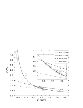
Figure 1: Pion form factor calculated directly from the interaction in Eq. (3): solid line. The data are from Refs. [References]. No parameters were varied to obtain the result. The other curves depict results from simplified calculations; in particular, the dash-dot line uses $\Gamma_{\mu}^{\gamma}(k;P)=\gamma_{\mu}$, which violates the Ward-Takahashi identity. (Adapted from Ref. [References].)

The same model can be employed without modification in calculating the impulse approximation to the light pseudoscalar meson form factors.[9, 10] In this application one needs additionally to solve the inhomogeneous vector vertex equation, which describes the dressed-quark–photon coupling and exhibits a pole at $P^{2}+m_{V}^{2}=0$; i.e., at the particular flavour channel’s vector meson mass. It is only by solving the inhomogeneous vertex equation that one can unambiguously evolve the form factor from the spacelike into the timelike region and vice versa.

The result for the pion form factor is illustrated in Fig. 1, with $r_{\pi}^{2}=(0.67\,{\rm fm})^{2}$ cf. expt.[15] $(0.663\pm 0.007\,{\rm fm})^{2}$. Good results are also obtained for the charged and neutral kaon form factors, with $r_{K^{+}}^{2}=(0.62\,{\rm fm})^{2}$ and $r_{K^{0}}^{2}=-(0.29\,{\rm fm})^{2}$ cf. expt.[15, 16] $r_{K^{+}}^{2}=(0.583\pm 0.043\,{\rm fm})^{2}$ and $r_{K^{0}}^{2}=-(0.23\pm 0.06\,{\rm fm})^{2}$. These results are too good because the calculations neglect meson-rescattering contributions that, in all channels, are additive in magnitude, with corrections of up to 15%.[17] Nevertheless they are a significant step, providing a manifestly Poincaré invariant calculation and unification of light-meson observables, with the particular feature that all calculated quantities are independent of the definition of the relative momentum, which is arbitrary in a covariant formulation. A three-dimensional reduction of the Bethe-Salpeter equation is unnecessary and is not employed. Furthermore, current conservation is automatic and the neutral mesons are neutral without fine-tuning. The same framework predicts:[18] $Q^{2}F_{\rm meson}(Q^{2})=\,$constant, as $Q^{2}\to\infty$, in accordance with the pQCD expectation, which is only possible because the pseudoscalar meson Bethe-Salpeter amplitude necessarily has pseudovector components.[19]

3   Nucleon Observables.  Reference [References] is an extensive study of the octet and decuplet baryon spectrum based on a quark-diquark Fadde^′ev equation. It represents the nucleon as a composite of a quark and pointlike diquark, which are bound together by a repeated exchange of roles between the dormant and diquark-participant quarks, and demonstrates conclusively that an accurate description of the spectrum is possible using these degrees of freedom. This motivates and supports the product Ansatz for the nucleon’s amplitude used in Refs. [References,References] to calculate a wide range of leptonic and nonleptonic nucleon form factors:

$$\Psi(p_{i};\alpha_{i},\tau_{i};\alpha,\tau)=\delta^{\tau\tau_{3}}\,\psi_{\alpha\alpha_{3}}(p_{1}+p_{2},p_{3})\Delta(p_{1}+p_{2})\,\Gamma_{\alpha_{1}\alpha_{2}}^{\tau_{1}\tau_{2}}(p_{1},p_{2})\,,$$ (5)

with the nucleon’s momentum: $P=p_{1}+p_{2}+p_{3}$, $P^{2}=-M^{2}$. In Eq. (5), $(\alpha_{i},\tau_{i})$ are quark spinor and isospin labels, and $(\alpha,\tau)$ are those of the nucleon, and

$$\psi_{\alpha\alpha_{3}}(\ell_{1},\ell_{2})=\delta_{\alpha\alpha_{3}}\psi_{1}(\ell^{2})-\frac{1}{M}\left(i\gamma\cdot\ell-\ell\cdot\hat{P}\delta_{\alpha\alpha_{3}}\right)\psi_{2}(\ell^{2})\,,$$ (6)

with $\ell=(1/3)\ell_{1}-(2/3)\ell_{2}$ and $\hat{P}^{2}=-1$, is a Bethe-Salpeter-like amplitude characterising the correlation between the quark and the diquark. In this form, $\psi_{1}$ describes the upper-component of the positive-energy nucleon spinor and $\psi_{2}$ the lower-component.[23] In addition, $\Delta(K)$ describes the pseudo-particle propagation characteristics of the diquark, and

$$\Gamma_{\alpha_{1}\alpha_{2}}^{\tau_{1}\tau_{2}}(p_{1},p_{2}) = (Ci\gamma_{5})_{\alpha_{1}\alpha_{2}}\,(i\tau^{2})^{\tau_{1}\tau_{2}}\,\Gamma(\ell^{2})\,,\;\ell=\mbox{\footnotesize$\displaystyle\frac{1}{2}$}q_{1}-\mbox{\footnotesize$\displaystyle\frac{1}{2}$}q_{2}\,,$$ (7)

represents the momentum-dependence, and spin and isospin character of the diquark correlation; i.e., it corresponds to a Bethe-Salpeter-like amplitude for what here is a nonpointlike diquark.

Equations (5)–(7) describe the nucleon as a composite of a quark and a scalar-diquark correlation, and in Refs. [References,References] the scalar functions were parametrised:

$$\begin{array}[]{ccc}\psi_{1}(\ell)=\frac{1}{{\cal N}_{\Psi}}\,{\cal F}(\ell^{2}/\omega_{\psi}^{2})\,,&\Gamma(\ell)=\frac{1}{{\cal N}_{\Gamma}}\,{\cal F}(q^{2}/\omega_{\Gamma}^{2})\,,&\Delta(K)=\frac{1}{m_{\Delta}^{2}}\,{\cal F}(K^{2}/\omega_{\Gamma}^{2})\,,\end{array}$$ (8)

${\cal F}(y)=(1-{\rm e}^{-y})/y$, $\psi_{2}=0$, with ${\cal N}_{\Psi}$ and ${\cal N}_{\Gamma}$ being the calculated nucleon and $(ud)$-diquark normalisation constants, which ensure composite electric charges of $1$ for the proton and $1/3$ for the diquark. The parameters $\omega_{\psi}=0.2\,$GeV, $\omega_{\Gamma}=1.4\,$GeV and $m_{\Delta}=0.63\,$GeV were fixed [22] in a least-squares fit to the proton’s charge form factor on $Q^{2}\in[0,3]\,$GeV². A good description is obtained and the parameter values demonstrate the internal consistency of the model. $d_{\Gamma}:=1/\omega_{\Gamma}$ is a measure of the mean separation between the quarks constituting the scalar diquark and $d_{\psi}:=1/\omega_{\psi}$ is the analogue for the quark-diquark separation. $d_{\Gamma}<d_{\psi}$ is necessary if the quark-quark clustering interpretation is to be valid. $\ell_{(ud)_{0^{+}}}=1/m_{\Delta}$ is a measure of the range over which the diquark may propagate and that must be significantly less than the nucleon’s diameter.

One particular highlight of the calculations is the result that the nonpointlike nature of the diquark allows a better description of the nucleons’ magnetic form factors than is possible in pointlike diquark models and, importantly, $|\mu_{n}/\mu_{p}|=0.55$ cf. expt. 0.68, whereas pointlike scalar-diquark models always yield $|\mu_{n}/\mu_{p}|<0.5$. Another is a prediction for the ratio $\mu_{p}G_{E}^{p}(q^{2})/G_{M}^{p}(q^{2})$ that is in semi-quantitative agreement with recent results from TJNAF.[24] A defect is that $|r_{n}^{2}|$ is 60% too large.

There are two obvious improvements – include: the lower component of the nucleon spinor, $\psi_{2}\neq 0$; and the axial-vector diquark. The first is underway and we report preliminary results for $\psi_{2}=\psi_{1}$. A fit to $G_{E}^{p}(p^{2})$ now requires

$$\begin{array}[]{l|ccc}&\;\omega_{\psi}&\;\omega_{\Gamma}&\;m_{\Delta}\\ \hline\cr\mbox{in GeV}&\;0.19&\;0.68&\;0.64\end{array}\,,\;\;\;\;\begin{array}[]{l|ccc}&\;1/\omega_{\psi}&\;1/\omega_{\Gamma}&\;1/m_{\Delta}\\ \hline\cr\mbox{in fm}&1.03&\;0.29&\;0.31\end{array}\,;$$ (9)

but this represents only a small change in the fitting parameters that preserves the model’s internal consistency [cf. after Eq. (8)]. These values yield

$$\begin{array}[]{c|ccccc}&\;r_{p}^{2}\,({\rm fm}^{2})&\;r_{n}^{2}\,({\rm fm}^{2})&\;\mu_{p}(\mu_{N})&\;\mu_{n}(\mu_{N})&\;\mu_{n}/\mu_{p}\\ \hline\cr{\rm Emp.}&(0.87)^{2}&-(0.34)^{2}&2.79&-1.91&-0.68\\ {\rm Calc.}&(0.78)^{2}&-(0.33)^{2}&2.81&-1.61&-0.57\\ \hline\cr\mbox{{\rm Old~{}Calc.\cite[cite]{[\@@bibref{}{jcrb1}{}{}]}}}&(0.79)^{2}&-(0.43)^{2}&2.88&-1.58&-0.55\\ \end{array}$$ (10)

and the recalculated neutron electric form factor in Fig. 2.

Figure 2: Solid line: neutron electric form factor calculated with $\psi_{2}=\psi_{1}$; i.e., including the lower component of the neutron spinor. Dashed line: the result with $\psi_{2}=0$.[21] Data from Ref. [References], extracted using the Argonne V18 potential.[26] Improving the product Ansatz, Eq. (5), by including $\psi_{2}$ significantly improves the estimate of $G_{E}^{n}$. However, this preliminary result is too good as we still ignore the axial vector diquark correlation.

As elucidated in Refs. [References], of these calculated quantities only $G_{E}^{n}$ involves a cancellation between contributions from the five diagrams that constitute the impulse approximation to the nucleon’s electromagnetic current in this model, and only observables tied to this form factor are dramatically affected by the improvement of the product Ansatz, Eq. (5). We anticipate that this is a general feature; i.e., only observables receiving interfering contributions; e.g., $g_{A}$ and the isoscalar tensor coupling $f_{\omega NN}$, are significantly modified by improvements. If this were not the case, simple models could not be generally efficacious.

Epilogue.  This overview is necessarily brief. It does no more than point to recent successes and says nothing of contemporary challenges. One such is to comprehend the origin of the infrared enhancement in the kernel of the QCD gap equation that is necessary to ensure DCSB. Another is to develop a BSE based understanding of the light scalar mesons and the $\eta$-$\eta^{\prime}$ mass-splitting. These aspects and more are canvassed in Ref. [References].

Acknowledgments.  CDR is grateful to the staff of the Special Research Centre for the Subatomic Structure of Matter at the University of Adelaide for their hospitality and support during this workshop, and in the two preceding weeks; and we acknowledge helpful communications with J.C.R. Bloch. This work was supported by the US Department of Energy, Nuclear Physics Division, under contract no. W-31-109-ENG-38, and benefited from the resources of the National Energy Research Scientific Computing Center. SMS is grateful for financial support from the A. v. Humboldt foundation.

References

References

- [1] C.D. Roberts, R.T. Cahill, M.E. Sevior and N. Iannella, Phys. Rev. D 49 (1994) 125.
- [2] M.A. Ivanov, Yu.L. Kalinovsky and C.D. Roberts, Phys. Rev. D 60 (1999) 034018.
- [3] D. Blaschke, C.D. Roberts and S.M. Schmidt, Phys. Lett. B 425 (1998) 232.
- [4] L. v. Smekal, A. Hauck and R. Alkofer, Annals Phys. 267 (1998) 1; D. Atkinson and J. C. Bloch, Mod. Phys. Lett. A 13 (1998) 1055.
- [5] F.T. Hawes, P. Maris and C.D. Roberts, Phys. Lett. B 440 (1998) 353.
- [6] M. Bando, M. Harada and T. Kugo, Prog. Theor. Phys. 91 (1994) 927; C.D. Roberts, Nucl. Phys. A 605 (1996) 475; P. Maris and C.D. Roberts, Phys. Rev. C 58 (1998) 3659.
- [7] P. Maris and C.D. Roberts, Phys. Rev. C 56 (1997) 3369.
- [8] P. Maris and P.C. Tandy, Phys. Rev. C 60 (1999) 055214.
- [9] P. Maris and P.C. Tandy, Phys. Rev. C 61 (2000) 45202.
- [10] P. Maris and P.C. Tandy, “The , and electromagnetic form factors,” nucl-th/0005015.
- [11] A. Bender, C.D. Roberts and L. v. Smekal, Phys. Lett. B 380 (1996) 7.
- [12] D. B. Leinweber, Annals Phys. 254 (1997) 328.
- [13] C. Caso et al., Eur. Phys. J. C 3 (1998) 1.
- [14] J.I. Skullerud and A.G. Williams, “The quark propagator in momentum space,” hep-lat/9909142; and these proceedings.
- [15] Open circles, C.J. Bebek et al., Phys. Rev. D 13 (1976) 25; Squares, L.M. Barkov et al., Nucl. Phys. B 256 (1985) 365; Filled circles, S.R. Amendolia et al. [NA7 Collaboration], Nucl. Phys. B 277 (1986) 168.
- [16] W. R. Molzon et al., Phys. Rev. Lett. 41 (1978) 1213.
- [17] R. Alkofer, A. Bender and C.D. Roberts, Int. J. Mod. Phys. A 10 (1995) 3319.
- [18] P. Maris and C.D. Roberts, Phys. Rev. C 58 (1998) 3659.
- [19] P. Maris, C.D. Roberts and P.C. Tandy, Phys. Lett. B 420 (1998) 267.
- [20] G. Hellstern, R. Alkofer, M. Oettel and H. Reinhardt, Nucl. Phys. A 627 (1997) 679.
- [21] J.C.R. Bloch, C.D. Roberts, S.M. Schmidt, A. Bender and M.R. Frank, Phys. Rev. C 60 (1999) 062201.
- [22] J.C.R. Bloch, C.D. Roberts and S.M. Schmidt, “Selected nucleon form factors and a composite scalar diquark,” nucl-th/9911068, to appear in Phys. Rev. C.
- [23] K. Kusaka, G. Piller, A.W. Thomas and A.G. Williams, Phys. Rev. D 55 (1997) 5299.
- [24] M.K. Jones et al. [Jefferson Lab Hall A Collaboration], Phys. Rev. Lett., 84, 1398 (2000).
- [25] S. Platchkov et al., Nucl. Phys. A 510 (1990) 740.
- [26] R.B. Wiringa, private communication; R.B. Wiringa, V.G. Stoks and R. Schiavilla, Phys. Rev. C 51 (1995) 38.
- [27] C.D. Roberts and S.M. Schmidt, “Density, Temperature and Continuum Strong QCD,” nucl-th/0005064.