=1 LAITH J. ABU-RADDAD dissertation Department of Physics Kirby W. Kemper Chairman Donald J. Foss Doctor of Philosophy 2000 Physics Jorge Piekarewicz Ph.D. Gregory Riccardi Simon Capstick Adam Sarty Adriana Moreo Summer Arts and Sciences APRIL 27, 2000 For my parents Huda and Jamal, my wife Mercedes, and my son Ommar.

PHOTOPRODUCTION OF PSEUDOSCALAR MESONS FROM NUCLEI

Acknowledgements       My dissertation could not have been achieved without the support, patience, and guidance of Professor Jorge Piekarewicz in every detail of this research work. I am deeply indebted for his close personal interaction and concern. My sincere thanks to every member of the Nuclear Theory Group at Florida State University for making this doctoral study such an educational and enjoyable experience. I would like also to extend my sincere appreciation to Professor Simon Capstick, Professor Adriana Moreo, Professor Gregory Riccardi, and Professor Adam Sarty for reviewing this manuscript.

This work was supported in part by the United States Department of Energy under Contracts Nos. DE-FC05-85ER250000 and DE-FG05-92ER40750.

ABSTRACT

Chapter 0 Introduction

Before describing my doctoral research I would like to point out that this manuscript has been written with the following philosophy in my mind: I aspire to provide the reader with a comprehensive overview of my research that stresses the fundamental physics and avoids unnecessary details. In many occasions, insignificant intricacies were sacrificed for a logical flow of ideas.

This research is concerned with the pseudoscalar meson photoproduction from nuclei. A meson is a particular kind of fundamental particle (as the pion, eta, and kaon) made up of a quark and an antiquark [1]. Quarks are the elementary particles that constitute, as we believe today, the fundamental building blocks of matter. Pseudoscalar mesons form a subgroup of mesons that have zero spin (and thus called scalars) and behave in a certain well-defined fashion under the action of symmetry operations. More specifically, the pseudoscalar-meson wavefunction $\phi$ transforms to $-\phi$ under the symmetry operation of spatial inversion. We study in this manuscript photoproduction processes of three pseudoscalar mesons: the kaon, pion, and eta. Table 1 illustrates the quark content of the different states of these mesons. In this table $u$, $d$, and $s$ stand for up, down, and strange quarks respectively, while $\bar{u}$, $\bar{d}$, $\bar{s}$ stand for the corresponding antiparticles (antiquarks) of these quarks.

Table 1: Quark content of the kaon, pion, and eta pseudoscalar mesons.

Pseudoscalar Meson	Quark	Content
Kaon	$K^{+}\sim\bar{s}u$	$K^{-}\sim\bar{u}s$
	$K^{\circ}\sim\bar{s}d$	$\bar{K}^{\circ}\sim\bar{d}s$
Pion	$\pi^{+}\sim\bar{d}u$	$\pi^{-}\sim\bar{u}d$
	$\pi^{\circ}\sim\frac{1}{\sqrt{2}}(\bar{u}u-\bar{d}d)$
Eta	$\eta\sim\frac{1}{\sqrt{6}}(\bar{u}u+\bar{d}d-2\bar{s}s)$

Photoproduction describes a process where elementary particles (such as mesons) are produced as a result of the action of photons (electromagnetic waves) on atomic nuclei [1]. The basic interaction in this work is as following: a photon is incident on a target nucleus and interacts with its constituents. As a result, a pseudoscalar meson is produced along with other particles. For simplicity, we investigate here photoproduction processes only from spherical nuclei. We study here two kinds of processes depending on the nature of the other particles produced in this interaction: coherent and quasifree processes.

In the coherent processes, the meson is produced with the target nucleus maintaining its initial character. Thus we start the interaction with a photon and some nucleus, and end up with a meson and the same nucleus we started with. The process is labeled “coherent” because all protons and neutrons (referred to collectively as “nucleons”) in the nucleus participate in the process, leading to a coherent sum of these individual nucleon contributions.

In the quasifree processes, the nucleus ruptures and thus fails to maintain its initial identity. The meson is produced in association with a nucleon (or an excited state of the nucleon like the lambda hyperon) and some new recoil “daughter” nucleus. Thus, we start the interaction with a photon and some nucleus, and end up with a meson, a free nucleon (or an excited state of it), and a new nucleus. The process is labeled as “quasifree” because it occurs in kinematic and physical circumstances similar to those of the process that produces a meson from a free unbound nucleon.

It is appropriate here to try to place these interactions to the bigger picture of general physics research. Studying these processes is one facet of the physicists’ quest to understand the fundamental strong force which plays the prominent role in interactions between elementary particles at very small distance scales. In our current understanding of physics, there are four forces that drive all interactions in nature: gravitational, electromagnetic, weak, and strong forces. Of these, we understand to a great extent the nature of the electromagnetic and the weak forces, while the gravitational and the strong still elude satisfactory and complete description. We do have a theory for the strong interactions — Quantum Chromodynamics (QCD) — but this theory is formidable to solve. As a result, a large chunk of the scientific research in physics today, whether in experiment or theory, is devoted to understanding this strong force. This effort is so extensive that it encompasses thousands of scientists in the fields of elementary particle and nuclear physics. This work is one minute step in this grand path, in the subfield called medium-energy nuclear physics. Our study attempts to provide a theoretical understanding of experiments that have been conducted or planned to be conducted in several laboratories: in the USA [such as the Thomas Jefferson National Accelerator Facility (TJNAF)], in Europe [such as the Mainz Microtron Laboratory (MAMI)], or in Japan [at the Research Center for Nuclear Physics (RCNP)].

The study I presented here assists in understanding several issues regarding this grand path of comprehending QCD. One of these is the structure and nature of the QCD bound states. There are two kinds of bound states in QCD: mesons (like the pion or the kaon), and hadrons, which includes nucleons (protons or neutrons) and nucleon resonances (excited states of nucleons) such as the lambda or delta particles. The processes of meson photoproduction are excellent tools in studying these states since these reactions proceed through the exchange of QCD bound states. For example, the pion photoproduction in a certain energy regime occurs as a result of the exchange of a delta resonance. By studying this process, we can have insights into the nature of this resonance and the mechanisms by which it interacts and decays.

Many research projects have been devoted to studying these kinds of meson photoproduction processes. Most studies have concentrated on studying the photoproduction from free nucleons. Such a process is labeled as “free” or “elementary” to distinguish it from the same process from a nucleus. An enormous amount of knowledge has been accumulated as a result, but this is still insufficient.

In this work, we go a step further by studying these processes from nuclei, because the nucleus in the coherent process acts as a “filter” that allows certain physical mechanisms that occur in the elementary process to go through, while blocking others. An example of this is the $S_{11}$ resonance that dominates the elementary process of eta photoproduction from a nucleon, but is almost perfectly suppressed in the process from a spherical nucleus due to this filtering. Thus, other mechanisms (such as the $D_{13}$ resonance) that are overshadowed by the $S_{11}$ and cannot be disentangled in the elementary process, in fact dominate the process from a nucleus. Another manifestation of this filtering is that the process from a spherical nucleus depends only on one of the four amplitudes that drive the elementary process. Indeed, the nucleus here acts as a laboratory to probe what we cannot study otherwise.

As the name conveys, the quasifree process from nuclei is the closest physically to the elementary or free process. The process can be viewed as the elementary one but now in a nuclear medium rather than in a free space. We can use this reaction to investigate the changes of the elementary process in the nuclear medium. One example is the pion quasifree process. As pointed out above, the pion elementary process is driven by delta resonance propagation in free space. In the quasifree process, however, this resonance propagates in a nuclear medium and so interacts through the strong force with the constituents of the nucleus, resulting in modifications to its basic properties. Understanding these modifications can elucidate some aspects of QCD.

So far I may have given an inaccurate impression that this work illuminates parts of our knowledge concerning only the “very small” scales of time and space. The processes that drive the “very small” also propel the “very large”. Indeed, our impetus to study the quasifree process is because it is a basic building block toward the bigger goal of assessing the possibility of kaon condensation in neutron stars. Neutron stars are dense celestial objects that consist primarily of closely packed neutrons and result from the collapse of a supernova [1]. These stars are among the most dense systems that we can find in nature; their densities are about ten times that of the nucleus, which is the most dense system in our solar system. Inquiries regarding the nature, structure, and stability of these objects are among the most intriguing questions in astrophysics today. One of the scenarios that may be able to explain their existence is that these stars consist of a new state of matter: strange matter. Strange matter refers to a form of matter where there is a significant presence of strange quarks. Although strange matter has been observed in laboratories — as in the production of hypernuclei — this matter has not yet been observed as a stable state in nature. Kaon condensation in neutron stars describes a hypothetical mechanism where, due to the very high density, it becomes energetically favorable to produce strange particles like the kaon (strange meson) or the lambda (strange nucleon resonance). Thus, we have a stable matter that is a “condensate” of “strangeness”. Much work has been devoted to this possibility and this scenario has yet to be confirmed or refuted conclusively.

The bulk of this dissertation is essentially a reproduction of several publications by the author and the collaboration [2, 3, 4, 5, 6]. Since it is tedious and pointless to keep referring to these publications throughout the manuscript, I only referred to them when I determine it to be appropriate to do so. The reader should bear in mind however that much of this work has its origin in these publications.

I would like to ask the reader for forgiveness for any repetitions in this manuscript. In several occasions, I had to repeat certain aspects because of appropriateness or significance in context.

Throughout this work (unless otherwise stated) we adopt the natural system of units where $\hbar=c=1$. This system is the appropriate and standard one in all studies involving quantum field theory.

1 Outline of Thesis

The dissertation is divided into three parts: preliminaries, coherent process, and quasifree process. The preliminaries part includes Chapters 1 and 2. Chapter 1 describes the basic ideas behind what is referred to as the elementary process: a pseudoscalar meson is photo-produced from a free nucleon. Understanding this process is the foundation for understanding the same process from nuclei. Since I will study processes from nuclei, I have to build the nuclear structure for several nuclei. This is done in Chapter 2, where a relativistic nuclear structure formalism is developed.

In the second part of the dissertation that encompasses Chapters 3, 4, 5, and 6, I concentrate on the coherent process. I study this process for two kinds of mesons: the pion ($\pi$) and the eta ($\eta$). In Chapter 3, I develop the basic theory where no final-state interactions are assumed between the emitted meson and the recoil nucleus. Then, I incorporate these interactions in Chapter 4. In Chapter 5, I present our results for this kind of process and discuss them. Finally in Chapter 6, I draw conclusions.

The third part of the manuscript follows in a similar fashion to the second one, but here I investigate the quasifree process. This is done in Chapters 7, 8, and 9. I study this interaction only for one kind of meson: the kaon ($K^{+}$). In Chapter 7, I sketch the theory behind this process, while I present and discuss the results in Chapter 8, and finally conclude in Chapter 9.

2 Technical Introduction and Background for the Coherent Process

The coherent photoproduction of pseudoscalar mesons has been advertised as one of the cleanest probes for studying how nucleon-resonance formation, propagation, and decay get modified in the many-body environment of nuclear matter; for current experimental efforts see Ref. [7]. The reason behind such optimism is the perceived insensitivity of the reaction to nuclear-structure effects. Indeed, many of the earlier nonrelativistic calculations suggest that the full nuclear contribution to the coherent process appears in the form of its matter density [8, 9, 10, 11, 12, 13]—itself believed to be well constrained from electron-scattering experiments and isospin considerations.

Recently, however, this simple picture has been put into question. Among the many issues currently addressed—and to a large extent ignored in all earlier analyses—are: background (non-resonant) processes, relativity, off-shell ambiguities, non-localities, and violations of the impulse approximation. We discuss each one of them in this manuscript. For example, background contributions to the resonance-dominated process can contaminate the analysis due to interference effects. This has been shown recently for the $\eta$-photoproduction process, where the background contribution (generated by $\omega$-meson exchange) is in fact larger than the corresponding contribution from the $D_{13}(1520)$ resonance [2]. We suggest in our study that—by using a relativistic and model-independent parameterization of the elementary amplitude—the nuclear-structure information becomes sensitive to off-shell ambiguities. Further, the local assumption implicit in most impulse-approximation calculations, and used to establish that all nuclear-structure effects appear exclusively via the matter density, has been lifted by Peters, Lenske, and Mosel [14, 15]. An interesting result that emerges from their work on coherent $\eta$-photoproduction is that the $S_{11}(1535)$ resonance—known to be dominant in the elementary process but predicted to be absent from the coherent reaction [10]—appears to make a non-negligible contribution to the coherent process in the case of non-spin-saturated but spherical nuclei such as ¹²C. Spin-saturated nuclei represent one type of nuclei where all states corresponding to one orbital angular momentum are completely filled. Finally, to our knowledge, a comprehensive study of possible violations to the impulse-approximation, such as the modification to the production, propagation, and decay of nucleon resonances in the nuclear medium, has yet to be done.

In this work we concentrate—in part because of the expected abundance of new, high-quality experimental data—on the coherent photoproduction of neutral pions. The central issue to be addressed here is the off-shell ambiguity that emerges in relativistic descriptions and its impact on extracting reliable resonance parameters; no attempt has been made here to conduct a quantitative and detailed study of possible violations of the impulse approximation or to the local assumption. These violations have been studied only qualitatively. Indeed, we carry out our calculations within the framework of a relativistic impulse approximation model. However, rather than resorting to a nonrelativistic reduction of the elementary amplitude, we keep intact its full relativistic structure [16]. As a result, the lower components of the in-medium Dirac spinors are evaluated dynamically in the Walecka model [17].

Another important ingredient of the calculation are the final-state interactions of the outgoing meson with the nucleus. We address the mesonic distortions via an optical-potential model of the meson-nucleus interaction. For example, we use earlier models of the pion-nucleus interaction plus isospin symmetry—since these models are constrained mostly from charged-pion data—to construct the neutral-pion optical potential. However, since we are unaware of a realistic optical-potential model that covers the $\Delta$-resonance region, we have extended the low-energy work of Carr, Stricker-Bauer, and McManus [18] to higher energies. In this way we have attempted to keep to a minimum the uncertainties arising from the optical potential, allowing concentration on the impact of the off-shell ambiguities to the coherent process.

3 Technical Introduction and Background for the Quasifree Process

Impelled by recent experimental advances, there is an increasing interest in the study of strangeness-production reactions from nuclei. These reactions form our gate to the relatively unexplored territory of hypernuclear physics. Moreover, these reactions constitute the basis for studying novel physical phenomena, such as the existence of a kaon condensate in the interior of neutron stars[19]. Indeed, the possible formation of the condensate could be examined indirectly by one of the approved experiments[20] at the Thomas Jefferson National Accelerator Facility (TJNAF). This experimental approach is reminiscent of the program carried out at the Los Alamos Meson Physics Facility (LAMPF) where pion-like modes were studied extensively through the quasifree $(\vec{p},\vec{n})$ reaction [21, 22]. These measurements placed strong constraints on the (pion-like) spin-longitudinal response and showed conclusively that the long-sought pion-condensed state does not exist.

The work presented here is a small initial step towards a more ambitious program that concentrates on relativistic studies of strangeness in nuclei. Our aim in this manuscript is the study of the photoproduction of kaons from nuclei in the quasifree regime. This investigation helps us in two fronts. First, it sheds light on the elementary process, $\gamma p\rightarrow K^{+}\Lambda$, by providing a different physical setting (away from the on-shell point) for studying the elementary amplitude. Second, it will enable us, in a future study, to explore modifications to the kaon propagator in the nuclear medium and to search for those observables most sensitive to the formation of the condensate. To achieve these goals we focus on the study of polarization observables. Polarization observables have been instrumental in the understanding of elusive details about subatomic interactions, as they are much more effective discriminators of subtle physical effects than the traditional unpolarized cross section. Moreover, quasifree polarization observables might be one of the cleanest tools for probing nuclear dynamics. For example, the reactive content of the process is simple, being dominated by the quasifree production and knockout of a $\Lambda$-hyperon. Further, free polarization observables provide a baseline, against which possible medium effects may be inferred. Deviations of polarization observables from their free values are likely to arise from a modification of the interaction inside the nuclear medium or from a change in the response of the target. Indeed, relativistic models of nuclear structure predict medium modifications to the free observables stemming from an enhanced lower component of the Dirac spinors in the nuclear medium [17]. Finally, nonrelativistic calculations of the photoproduction of pseudoscalar mesons suggest that, while distortion effects provide an overall reduction of the cross section, they do so without substantially affecting the shape of the distribution[23, 24, 25]. Indeed, these nonrelativistic calculations show that two important polarization observables — the recoil polarization of the ejected baryon and the photon asymmetry — are largely insensitive to distortion effects. Moreover, they seem to be also independent of the mass of the target nucleus.

An insensitivity of polarization observables to distortion effects is clearly of enormous significance, as one can unravel distortion effects from those effects arising from relativity or from the large-momentum components in the wavefunction of the bound nucleon. Indeed, relativistic plane-wave impulse approximation (RPWIA) calculations have been successful in identifying physics not present at the nonrelativistic level [26, 27]. Finally, neglecting distortions allows the computation of all polarization observables in closed form [26] by using the full power of Feynman’s trace techniques.

Chapter 1 Photoproduction of pseudoscalar mesons from free nucleons

Any investigation of the processes of meson photoproduction from nuclei must start with a study of the photoproduction from a single free nucleon. This process from a free nucleon is usually labeled as elementary to distinguish it from other processes from an interacting or bound nucleon. It is appropriate here to stress that it is not the purpose of this work to investigate the photoproduction interactions from free nucleons; this topic has been extensively studied by many scientific groups and is an “industry” of its own. It is imperative, however, to examine these processes to incorporate them in our investigation of the photoproduction reactions from nuclei. We start this chapter by describing the basic formalism of any elementary process of meson photoproduction from a free nucleon.

1 Elementary Process: Model Independent Formalism

In the elementary process a photon is absorbed by a free nucleon (a proton or a neutron) to yield a pseudoscalar meson in addition to a nucleon (or a hyperon). Figure 1 illustrates this process.

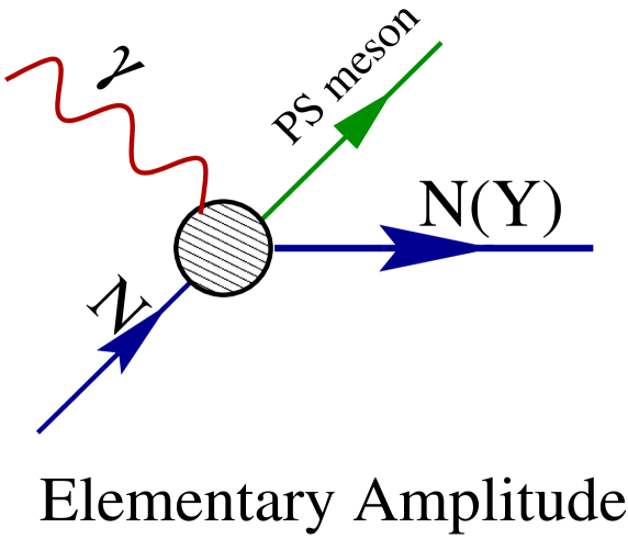
Figure 1: The elementary process of pseudoscalar meson photoproduction from a single free nucleon. A photon is absorbed by the nucleon to yield a pseudoscalar meson in addition to a nucleon (or a hyperon).

The most general expression for the scattering matrix element using perturbation theory can be written as a multiple integral in the following form:

$$\int d^{4}x_{1}\ldots d^{4}x_{N}\;\overline{{\psi}}A^{\mu}J_{\mu}(x_{1},\ldots,x_{N}){\psi}\phi\;,$$ (1)

where $\psi$ is the Dirac spinor for a free nucleon, $A^{\mu}$ is the photon wavefunction (field), and $\phi$ is the pseudoscalar meson wavefunction (field). The expression clearly includes the electromagnetic contraction between the photon field and the conserved electromagnetic current $J_{\mu}(x_{1},...,x_{N})$. The number $N$ of independent variables to be integrated over, depends on the nature of the effective field theory employed. In other words, it depends on the number of vertices in each Feynman diagram derived from this effective field theory. From this most general form, it can be shown that the model independent parameterization for this interaction is given in terms of four Lorentz- and gauge-invariant amplitudes (matrices) in the space of Dirac spinors as[10, 16, 28, 29]

$$T[\gamma N\rightarrow PS\,meson\,N(Y)]=\sum_{i=1}^{4}A_{i}(s,t)M_{i}\,,$$ (2)

where the invariant matrices have the form

$$M_{1} = -\gamma^{5}\hbox to0.0pt{/\hss}{\varepsilon}\hbox to0.0pt{/\hss}k\,,$$

$$M_{2} = 2\gamma^{5}[(\varepsilon\cdot p_{1})(k\cdot p_{2})-(\varepsilon\cdot p_{2})(k\cdot p_{1})]\,,$$

$$M_{3} = \gamma^{5}[\hbox to0.0pt{/\hss}{\varepsilon}((k\cdot p_{1})-\hbox to0.0pt{/\hss}k(\varepsilon\cdot p_{1})]\,,$$

$$M_{4} = \gamma^{5}[\hbox to0.0pt{/\hss}{\varepsilon}((k\cdot p_{2})-\hbox to0.0pt{/\hss}k(\varepsilon\cdot p_{2})]\,,$$ (3)

and where $\varepsilon$ and $k$ are the polarization and four-momenta of the photon, and ${p_{1}}$ and ${p_{2}}$ are the four momenta of the struck nucleon and recoil nucleon (hyperon) respectively. The terms $\hbox to0.0pt{/\hss}{\varepsilon}$ and $\hbox to0.0pt{/\hss}k$ stand for $\gamma^{\mu}\varepsilon_{m}u$ and $\gamma^{\mu}k_{\mu}$ respectively. Here, the kinematic quantities $s$ and $t$ are the Mandelstam variables $s\equiv(p_{1}+k)^{2}$ and $t\equiv(k-k^{\prime})^{2}$.

This is the standard, but not unique, parameterization of the elementary process. There are many other possible parameterizations which are equivalent provided the struck nucleon is free (on-shell). Unfortunately, it is not clear how we can apply this parameterization to a bound nucleon (off-shell nucleon) without a detailed microscopic model for this process. We will come back to this point in Chapter 3.

We choose to transform this standard form into a more suitable one[2] by using the identity[30]

$$\gamma^{5}\gamma^{\mu}\gamma^{\nu}=\gamma^{5}g^{\mu\nu}+\frac{1}{2i}\varepsilon^{\mu\nu\alpha\beta}\gamma_{\alpha}\gamma_{\beta}\,,$$ (4)

to rewrite the term $M_{1}=-\gamma^{5}\hbox to0.0pt{/\hss}{\varepsilon}\hbox to0.0pt{/\hss}k$ as

$$M_{1} = -\gamma^{5}\hbox to0.0pt{/\hss}{\varepsilon}\hbox to0.0pt{/\hss}k$$ (5)

$$= \frac{1}{2}\varepsilon^{\mu\nu\alpha\beta}\varepsilon_{\mu}k_{\nu}\sigma_{\alpha\beta}\,,$$ (6)

where we have used the convention of $\varepsilon^{0123}=-1$ for the Levi-Civita tensor. Consequently, the parameterization of the elementary process is rewritten as

$$T[\gamma N\rightarrow PS\,meson\,N(Y)]=F^{\alpha\beta}_{T}\sigma_{\alpha\beta}+F_{P}i\gamma_{5}+F^{\alpha}_{A}\gamma_{\alpha}\gamma_{5}\,,$$ (7)

where tensor, pseudoscalar, and axial-vector coefficients have been introduced as following

$$F^{\alpha\beta}_{T} = \frac{1}{2}\varepsilon^{\mu\nu\alpha\beta}\varepsilon_{\mu}k_{\nu}A_{1}(s,t)\,,$$

$$F_{P} = -i\mbox{ }2\mbox{ }[(\varepsilon\cdot p_{1})(k\cdot p_{2})-(\varepsilon\cdot p_{2})(k\cdot p_{1})]A_{2}(s,t)\,,$$

$$F^{\alpha}_{A} = [(\varepsilon\cdot p_{1})k^{\alpha}-(k\cdot p_{1})\varepsilon^{\alpha}]A_{3}(s,t)+[(\varepsilon\cdot p_{2})k^{\alpha}-(k\cdot p_{2})\varepsilon^{\alpha}]A_{4}(s,t)\,.$$ (8)

This form manifests nicely the Lorentz and parity transformation properties of the different bilinear covariants.

2 Elementary Process: Model Dependent Formalism

The parameterization developed above is model independent and applies to any process of pseudoscalar meson photoproduction from a single free nucleon. This parameterization, however, is in terms of four unknown amplitudes: $\{A_{1},A_{2},A_{3},A_{4}\}$. These amplitudes can be determined using different methods. In one method, we can simply extract them from experimental data for the observables of these processes. Another method, which is a fundamental one, is to study the physical processes behind each photoproduction process, and thus to construct a microscopic model for this process in terms of the fundamental degrees of freedom in this interaction. Since these degrees of freedom involve quarks and gluons, this approach is simply intractable at this point. An alternative approach is to build a microscopic model that accommodates all the symmetries of the problem while describing the interaction in terms of effective degrees of freedom. This is in fact what is done by many researchers in this field using effective Lagrangian field theories.

In an effective Lagrangian field theory, one postulates a Lagrangian that encompasses physically reasonable degrees of freedom. Then from this Lagrangian one finds the field equations of the system. Since solving these equations is still obstinate, one resorts to perturbation theory to determine the dynamics of the system. This involves the generation of Feynman diagrams describing the process. By calculating these diagrams we can determine the observables. From experimental data for these observables, one fits the unknown parameters in the effective theory. In the following three subsections, I will present briefly three effective Lagrangian theories for the photoproduction of $\eta$, $\pi$, and $K$ mesons respectively from a free nucleon.

1 Eta Photoproduction from a Free Nucleon: $N(\gamma,\eta)N$

This process is assumed to proceed in the s- and u-channels through the exchange of nucleons (Born terms) and nucleon excited states (resonances) like the $S_{11}(1535)$ and $D_{13}(1520)$ resonances [2, 15, 31, 32]. In the t-channel we have vector-meson exchanges like the $\omega$ and $\rho$ mesons. Figure 2 lists the Feynman diagrams for this process.

Figure 2: The $\eta$ photoproduction process from a free nucleon: $N(\gamma,\eta)N$. The process proceeds through the exchange of nucleons and resonances in the s- and u-channels, as well as vector-meson exchanges in the t-channel.

Of all of these diagrams, it turns out that the process is strongly dominated by only one of them: the s-channel resonance diagram in terms of the $S_{11}(1535)$ resonance. This contribution overshadows all other Feynman diagrams. Figure 3 illustrates this dominance where measurements are shown of the differential cross section as a function of incident-photon energy and at different scattering angles for this process from a proton or a neutron [2].

Figure 3: The differential cross section as a function of incident-photon energy at different scattering angles for the processes $p(\gamma,\eta)p$ and $n(\gamma,\eta)n$ [2]. The figure includes the theoretical calculations for this process with all Feynman diagram contributions included (Full Amplitude), and with only the $S_{11}(1535)$ resonance contribution ($S_{11}(1535)$ only). It also includes experimental measurements for these processes from Ref.’s  [33] (proton) and  [34] (extracted neutron).

The figure also includes the theoretical calculations for the differential cross section with all Feynman diagram contributions included (Full Amplitude), and with only the $S_{11}(1535)$ resonance contribution. It is clear that the $S_{11}(1535)$ alone can almost explain the total magnitude of the cross section.

2 Pion Photoproduction from a Free Nucleon: $N(\gamma,\pi)N$

In a similar fashion to the $\eta$ elementary process, one can develop an effective field theory for the pion photoproduction from a free nucleon. Then, we find that the $\eta$ and $\pi$ processes have similar Feynman diagrams, but in the case of the pion it is the $\Delta$ resonance that dominates this interaction [11, 14]. Figure 4 lists the different Feynman diagrams for this process.

Figure 4: The $\pi$ photoproduction process from a free nucleon: $N(\gamma,\pi)N$. The process proceeds through the exchange of nucleons and resonances in the s- and u-channels, as well as vector-meson exchanges in the t-channel.

Finally, we chose to extract the the amplitudes $A_{1},A_{2},A_{3},$ and $A_{4}$ from experimental data using the most recent phase-shift analysis of Arndt, Strakovsky, and Workman [35].

3 Kaon Photoproduction from a Free Nucleon: $p(\gamma,K^{+})\Lambda$

The microscopic model for the $K^{+}$ elementary process is somewhat different from the one for the $\eta$ (or $\pi$) meson. The reason is that we have here a strangeness production in the final state: a $\Lambda$ hyperon (strange nucleon) and a $K^{+}$ (strange meson) have been formed. These two particles have a net strange-quark content and thus labeled as strange particles. As a result of this strangeness production, the u and t-channels have to proceed now through strange particles. Thus we have a u-channel proceeding through the exchange of hyperons like the $\Lambda$ or $\Sigma$, as well as through resonances of these hyperons ($Y^{*}$), while the t-channel proceeds through the exchange of strange scalar mesons [28, 29, 36]. Figure 5 lists the different Feynman diagrams for this process.

Figure 5: The $K^{+}$ photoproduction process from a free nucleon: $p(\gamma,K^{+})\Lambda$. The process proceeds through the exchange of nucleons and resonances in the s-channel, through the exchange of hyperons like $\Lambda$ and $\Sigma$ and their resonances $Y^{*}$ in the u-channel, as well as strange-meson exchanges in the t-channel.

Chapter 2 Relativistic Nuclear Structure

Relativistic nuclear structure formalisms represent a growing field of study where the nuclear structure is determined using fully relativistic models. It has been argued for a long time that due to the relatively small binding of the nucleons in nuclei, nonrelativistic formalisms should be adequate to describe the nuclear structure. This assertion is impressively challenged in the relativistic treatments, where it has been suggested that the small binding energy is a result of a cancellation between two large potentials with different Lorentz transformation properties, with one of the potentials being attractive and the other repulsive.

Not only do the relativistic formalisms point to the importance of relativistic effects, but they also provide us with a more credible and aesthetic theory. This is because the relativistic formalism is an effective field theory as opposed to the “ad hoc” potential-based nonrelativistic formalisms. Thus the theory is physical and consistent with quantum-field-theory principles. Furthermore, aspects of the nuclear force that have always been put in the nonrelativistic formalisms by hand and with no basis, appear naturally in the relativistic formalisms. Examples of these include spin-orbit coupling and three-body forces.

Relativistic treatments have enjoyed a great success in recent years in their description of the nuclear structure. They do have a number of pitfalls that are systematically being surmounted and resolved. The bottom line, however, lies in the experimental verification of these formalisms. To this end, there are various experimental approaches that may decisively prove the validity and applicability of these formalisms.

1 Quantum Hadrodynamics

Quantum hadrodynamics (QHD) is a model for the study of the relativistic nuclear many-body problem through an effective Lagrangian field theory. The model was introduced by J. D. Walecka in 1974 [17]. It describes nuclear matter as resulting from interactions between nucleons (baryons) in the nucleus through the exchange of neutral scalar $\sigma$ and vector $\omega$ mesons. The couplings of these mesons to the baryon fields is achieved by the minimal substitution as can be seen in Table 1. In this table, $g_{s}$ is the scalar coupling constant and $g_{v}$ is the vector coupling constant. The model suggests a nucleon-nucleon force which is attractive at large separations and repulsive at short ones. Other mesons can be included in this formalism but their contributions are rather small — at least in the mean-field picture which we adopt here. For example, the contribution of the pion vanishes in the mean-field approximation as a result of its negative parity.

Table 1: The fields in quantum hadrodynamics.

Field	Description	Particle	Mass	Coupling
$\psi$	Baryon	p, n,…	$M$
$\phi$	Neutral scalar meson	$\sigma$	$m_{s}$	$g_{s}\bar{\psi}\phi\psi$
$V_{\mu}$	Neutral vector meson	$\omega$	$m_{v}$	$g_{v}\bar{\psi}\gamma^{\mu}V_{\mu}\psi$

The Lagrangian for this system is as following:

$${\cal L}={\bar{\psi}}[\gamma_{\mu}(i\partial^{\mu}-g_{v}V^{\mu})-(M-g_{s}\phi)]\psi+\frac{1}{2}(\partial_{\mu}\phi\partial^{\mu}\phi-m_{s}^{2}\phi^{2})-\frac{1}{4}F_{\mu\nu}F^{\mu\nu}+\frac{1}{2}m_{v}^{2}V_{\mu}V^{\mu}\,,$$ (1)

where

$$F_{\mu\nu}\equiv\partial_{\mu}V_{\nu}-\partial_{\nu}V_{\mu}\,.$$ (2)

The field equations can be derived then from the Lagrangian and one obtains

$$(\partial_{\mu}\partial^{\mu}+{m_{s}}^{2})\phi=g_{s}{\bar{\psi}}\psi\,,$$ (3)

$$(\partial_{\mu}\partial^{\mu}+{m_{v}}^{2})V^{\nu}=g_{v}{\bar{\psi}}\gamma^{\nu}\psi\,,$$ (4)

$$[\gamma_{\mu}(i\partial^{\mu}-g_{v}V^{\mu})-(M-g_{s}\phi)]\psi=0\,.$$ (5)

Hence we have a system of three coupled nonlinear differential equations. Since solving these equations exactly is a formidable task, one resorts to approximations like the mean-field picture known also as the Hartree approximation. In this picture, the scalar and vector fields are treated as classical fields, and one solves this system by finding the configuration of these fields that solves all three equations simultaneously. That is one finds a self-consistent solution for this system. As a result, the nucleon equation 5 becomes a one-body Dirac equation with a scalar $g_{s}\phi$ and a vector $g_{v}V^{\mu}$ potentials. One also finds that the spatial components of the vector field have a vanishing contribution in the static limit as a result of current conservation. This is because we are restricting our discussion to spherically symmetric nuclei with a total angular momentum of zero. The mean-field equation then reads as

$$[i\gamma^{\mu}\partial_{\mu}-g_{v}\gamma^{0}V({\mathbf{x}})-(M-g_{s}\phi({\mathbf{x}}))]\psi=0\,.$$ (6)

The theory has three free parameters to be determined: $\{g_{s},g_{v},m_{s}\}$; the $m_{v}$ is chosen as the physical mass of $\omega$ meson since this neutral vector meson is the natural degree of freedom in this effective field theory. These are resolved using basic properties of finite nuclei and infinite matter like the saturation density and the rms charge radius of ⁴⁰Ca.

In using the QHD model (known also as Walecka model) one finds that it can successfully explain and predict many physical features of nuclei with impressively a minimal number of phenomenological parameters that are determined from only bulk properties of nuclei. The relativistic structure is a keystone of this model. There are many consequences of this relativistic treatment [17]. One of them is the existence of a nuclear shell model with the experimentally observed level orderings, spacings, and major shell closures in nuclei.

Another consequence is the saturation of nuclear matter. This saturation explains the stability of only a limited number of nuclei which is what is observed in nature. The relatively small nuclear binding energy of saturation is the result of a very delicate and fine cancellation between a large scalar attraction and a large vector repulsion.

A third consequence of the relativistic structure is the spin-orbit splitting. The splitting here appears naturally and within the structure of the theory unlike the nonrelativistic treatments. In fact, we find a large spin-orbit splitting in this model as is experimentally verified.

A final consequence of this model is the density dependence of the interaction as the vector and scalar potentials have different density dependences. This difference is the reason for the nuclear saturation in this model. In the nonrelativistic treatments the density dependence must be included phenomenologically.

The natural remarkable consequences of the QHD Hartree model testify to its physical validity and to the “smartness” of the Dirac equation which, within its simple but illusive structure, can produce many physical effects that are never dreamed of in the nonrelativistic treatments.

2 Extensions to Quantum Hadrodynamics

Since Walecka introduced the QHD model many extensions have been achieved to improve its predictions. As a result, the original QHD model presented above is now labeled as QHD-I. One extension is the QHD-II introduced by Serot [17] that incorporates charged vector ${\rho}$ and charged pseudoscalar ${\pi}$ mesons in addition to the $\sigma$ and $\omega$ mesons. The model also incorporates the electromagnetic interaction through the photon field $A^{\mu}$ to account for the Coulomb repulsion between protons in nuclei. Table 2 lists the ingredients of this model.

Table 2: The fields in QHD-II.

Field	Description	Particle	Mass	Coupling
$\psi$	Baryon	p, n,…	$M$
$\phi$	Neutral scalar meson	$\sigma$	$m_{s}$	$g_{s}\bar{\psi}\phi\psi$
$V_{\mu}$	Neutral vector meson	$\omega$	$m_{v}$	$g_{v}\bar{\psi}\gamma^{\mu}V_{\mu}\psi$
${\pi}$	Charged pseudoscalar meson	$\pi$	$m_{\pi}$	$ig_{\pi}\bar{\psi}\gamma^{5}\mbox{\boldmath$\tau\cdot{\pi}$\unboldmath}\psi$
${\mathbf{b}_{\mu}}$	Charged vector meson	$\rho$	$m_{\rho}$	$\frac{1}{2}g_{\rho}\bar{\psi}\gamma^{\mu}$ $\tau\cdot{b_{\mu}}$$\psi$
${A_{\mu}}$	Photon	$\gamma$	$m_{\gamma}=0$	$e\bar{\psi}\gamma^{\mu}\frac{1}{2}(1+\tau_{3})A_{\mu}\psi$

Other extensions that incorporate nonlinear terms for the meson fields have also been introduced. QHD theory with these extensions provide us today with a very successful model for describing nuclear matter in an impressively transparent formalism. For the sake of brevity I will not elaborate on these extensions but it is appropriate to mention that I use only two versions of the QHD theory throughout this work namely QHD-I and QHD-II.

Finally, we have used a standard set of parameters for the Walecka model: $g_{s}^{2}=109.63$, $g_{v}^{2}=190.43$, $g_{\rho}^{2}=65.23$, $m_{s}=520$ MeV, $m_{v}=783$ MeV, and $m_{\rho}=770$ MeV.

3 Mean Field Approximation to ⁴He

In our study of meson photoproduction processes we have used ⁴He as a nuclear target. In doing so, we needed to have a reasonable description of the nuclear structure of ⁴He. We determined this structure using a mean-field approximation to the Walecka model. Even though the use of this approximation to describe a nucleus as small as ⁴He should be suspect, we feel justified in adopting this choice. The reason is that the photoproduction processes we studied are sensitive only to the bulk properties of ⁴He — which can be constrained by experiment. Consequently, in order to reproduce the experimental charge density of ⁴He, we have modified the mass of the $\sigma$ meson to $m_{s}=564$ MeV — while keeping constant the ratio of $g_{s}^{2}/m_{s}^{2}$. Figure 1 shows the ⁴He form factor (the Fourier transform of the proton density normalized to one)

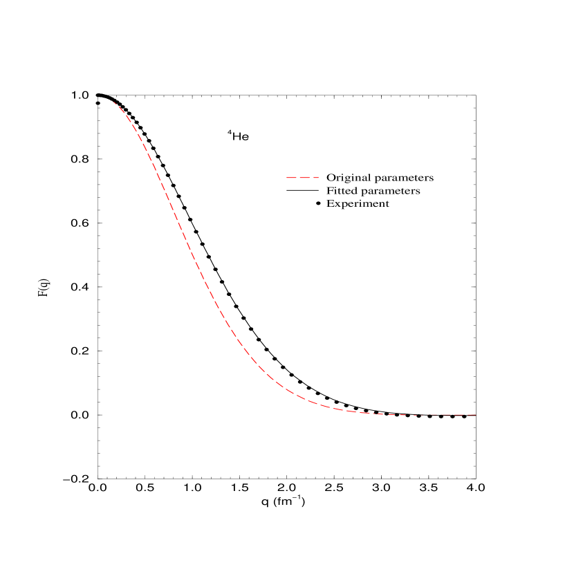
Figure 1: The ⁴He form factor as calculated using the original parameters of Walecka model (QHD-II), and then using the modified ones to fit the experimental form factor.

as a function of momentum transfer ($q\equiv|{\bf q}|$) as calculated using the original parameters of Walecka model (QHD-II), and then using the modified ones, to fit the experimental form factor (included also in the figure). It is remarkable that by a small change in only one of the parameters, we can fit the experimental form factor almost perfectly. To be noted here that the calculation using QHD-I gives also identical results to the QHD-II ones.

The experimental form factor (in the rest frame of the nucleus) in Figure 1 is produced using a phenomenological fit to data over a wide range of momentum transfers and is parameterized according to the following equation [9, 10]:

$$F(q)=-\frac{3\pi b\left[cos(qc)-\pi b\,sin(qc)\,coth(\pi bq)/c\right]}{qc^{2}sinh(\pi bq)[1+\pi^{2}b^{2}/c^{2}]}\;.$$ (7)

Here the parameters $b$ and $c$ are given in Table 3 for the three nuclei: ⁴He, ¹²C and ⁴⁰Ca.

Table 3: Parameters of the nuclear form factor for ⁴He, ¹²C, and ⁴⁰Ca.

	$b$ (fm)	$c$ (fm)
4He	0.406	1.231
12C	0.478	2.220
40Ca	0.537	3.573

4 Bound Nucleon Wavefunction

As evident in the previous sections, the QHD theory reduces to finding a solution to the nucleon Dirac equation 5 with scalar and vector potentials in such away that this solution is also self-consistent with the field equations 3 and 4. It is proper here to give a brief idea of the solutions to the Dirac equation with scalar and vector fields.

Concentrating on spherically symmetric nuclei one finds that the fields $\phi$ and $V^{0}$ must be spherically symmetric too. Hence, we can rewrite equation 5 for a certain energy eigenvalue $E$ with the new definitions of $S(r)=g_{s}\phi(r)$ and $V(r)=g_{v}V^{0}(r)$ as

$$H\psi=E\psi\,,$$ (8)

where

$$H=\mbox{\boldmath$\alpha\cdot p$\unboldmath}+\beta\left[\,M-S(r)\,\right]+V(r)\,.$$ (9)

In this equation

$$\alpha_{i}\equiv\gamma_{0}\gamma_{i}\,,$$ (10)

and

$$\beta\equiv\gamma_{0}\,.$$ (11)

We can find a set of commuting operators that also commute with the Hamiltonian ($H$) of this equation. Consequently, these operators provide us with constants of the motion that can be used to characterize the energy eigenfunctions. Examples of these operators include ${\mathbf{J}^{2}}$ (total angular momentum squared), $J_{z}$ (z-axis projection of the total angular momentum), and $K$  [37] an operator that is defined as

$$K\equiv\beta(2{{\mathbf{S}}\cdot{\mathbf{J}}}-\frac{1}{2})=\beta({2{\mathbf{S}}\cdot{\mathbf{L}}}+1)\,.$$ (12)

The operator $K$ determines in the nonrelativistic limit whether the projection of the spin is parallel or anti-parallel to the total angular momentum. The eigenvalues for these operators are $j(j+1)$ for ${\mathbf{J}^{2}}$, $m$ for $J_{z}$, and $-\kappa$ for $K$.

It can be shown that there is a relationship between $\kappa$ and $j$ which is

$$\kappa=\pm(j+\frac{1}{2})\,.$$ (13)

Hence $\kappa$ is a nonzero integer which can be positive or negative. The sign of $\kappa$ determines whether the spin is parallel (positive) or anti-parallel (negative) in the nonrelativistic limit.

We can write the four-component eigenfunction $\psi$ as a vector of two-component spinors

$$\psi={\psi_{A}\choose\psi_{B}}\,.$$ (14)

By this decomposition one can show that even though the four component eigenfunction is not an eigenfunction of ${\mathbf{L}^{2}}$, the spinors $\psi_{A}$ and $\psi_{B}$ are separately eigenfunctions with eigenvalues $l_{A}(l_{A}+1)$, and $l_{B}(l_{B}+1)$ respectively. It can be shown also that these eigenvalues are related to $\kappa$ and $j$ through the equations

$$-\kappa=j(j+1)-l_{A}(l_{A}+1)+\frac{1}{4}\,,$$ (15)

and

$$\kappa=j(j+1)-l_{B}(l_{B}+1)+\frac{1}{4}\,.$$ (16)

As a result any energy eigenfunction can be uniquely characterized by only $E$, $\kappa$, and $m$.

The above analysis enables us to write $\psi$ as

$$\psi={\psi_{A}\choose\psi_{B}}={g_{E\kappa}(r){y}{{}^{m}_{jl_{A}}}\choose if_{E\kappa}(r){y}{{}^{m}_{jl_{B}}}}\,,$$ (17)

where ${y}{{}^{m}_{jl}}$ are the normalized spin-angular functions constructed by the addition of Pauli spinors to the spherical harmonics of order $l$. The inclusion of $i$ with $f_{E\kappa}(r)$ is in order to make $f_{E\kappa}(r)$ and $g_{E\kappa}(r)$ real for bound-state solutions. Substituting this result back into the Dirac equation and performing some algebra, we arrive at the coupled equations:

$$-\frac{df}{dr}-\frac{(1-\kappa)}{r}f(r)=\left[E-V(r)-M+S(r)\,\right]g(r)\,,$$ (18)

$$\frac{dg}{dr}+\frac{(1+\kappa)}{r}g(r)=\left[E-V(r)+M-S(r)\,\right]f(r)\,.$$ (19)

Now writing these equations in terms of

$$F(r)=rf(r)\,,$$ (20)

$$G(r)=rg(r)\,,$$ (21)

we have

$$\frac{dF}{dr}-\frac{\kappa}{r}F(r)=-\left[E-V(r)-M+S(r)\,\right]G(r)\,,$$ (22)

$$\frac{dG}{dr}+\frac{\kappa}{r}G(r)=\left[E-V(r)+M-S(r)\,\right]F(r)\,.$$ (23)

These are two coupled differential equations which can be solved numerically by the Runge-Kutta method. It is worth noting that there is an implicit symmetry in these equations as $F\rightarrow G$ and $G\rightarrow F$ if $E\rightarrow-E$, $V(r)\rightarrow-V(r)$, and $\kappa\rightarrow-\kappa$.

5 Nuclear Densities in the Relativistic Formalism

Nuclear densities in the relativistic formalisms are a vivid example of the richness of relativity. While we have essentially only one ground state density in the nonrelativistic formalisms: the vector (matter) density, the relativistic treatments provide us with the possibility of having up to five different densities: vector (matter), tensor, scalar, axial-vector, and pseudoscalar. This richness is a result of the fact that in the space of Dirac spinors we can have up to 16 linearly-independent matrices. These form the set: $\{1,\gamma^{\mu},\gamma^{\mu}\gamma^{5},i\gamma^{5},\sigma^{\mu\nu}\}$ of bilinear covariants. The covariants transform as scalar, vector, axial-vector, pseudoscalar, and tensor respectively under Lorentz transformations (Poincaré group). It is important to note that the densities are truly independent and constitute fundamental nuclear-structure quantities. The fact that in the nonrelativistic framework only one density survives is due to the limitation of the approach. Indeed, in the nonrelativistic framework one employs the free space relation to relate the lower to the upper component of the Dirac spinor instead of determining the lower component dynamically through the Dirac equation. Hence, any evidence of possible medium modifications to the ratio of lower-to-upper components of the Dirac spinors is lost.

Using the QHD theory developed above one finds that there are three non-vanishing ground state densities for spherical and spin-saturated nuclei. These are the conventional matter (vector) density defined by

$$\rho_{\lower 3.0pt\hbox{$\scriptstyle V$}}(r)=\sum_{\alpha}^{\rm occ}\overline{{\cal U}}_{\alpha}({\bf x})\,\gamma^{{\scriptscriptstyle 0}}\,{\cal U}_{\alpha}({\bf x})\,,\quad$$ (24)

which leads to the vector density given by

$$\rho_{\lower 3.0pt\hbox{$\scriptstyle V$}}(r)=\sum_{a}^{\rm occ}\left({2j_{a}+1\over 4\pi r^{2}}\right)\Big{(}g_{a}^{2}(r)+f_{a}^{2}(r)\Big{)}\,,$$ (25)

where ${\cal U}_{\alpha}({\bf x})$ is a single-particle Dirac spinor (solution to Dirac equation) for the bound nucleon, $g_{a}(r)$ and $f_{a}(r)$ are the radial parts of the upper and lower components of the Dirac spinor, respectively, and the above sums run over all the occupied single-particle states in the nucleus. Analogously, the scalar density is defined by

$$\rho_{\lower 3.0pt\hbox{$\scriptstyle S$}}(r)=\sum_{\alpha}^{\rm occ}\overline{{\cal U}}_{\alpha}({\bf x})\,{\cal U}_{\alpha}({\bf x})\,,\quad$$ (26)

leading to it given as

$$\rho_{\lower 3.0pt\hbox{$\scriptstyle S$}}(r)=\sum_{a}^{\rm occ}\left({2j_{a}+1\over 4\pi r^{2}}\right)\Big{(}g_{a}^{2}(r)-f_{a}^{2}(r)\Big{)}\,.$$ (27)

Finally, we have the tensor density defined by

$$\Big{[}\rho_{\lower 3.0pt\hbox{$\scriptstyle T$}}(r)\,\hat{r}\Big{]}^{i}=\sum_{\alpha}^{\rm occ}\overline{{\cal U}}_{\alpha}({\bf x})\,\sigma^{{\scriptscriptstyle 0}i}\,{\cal U}_{\alpha}({\bf x})\,,\quad$$ (28)

resulting in the following expression for $\rho_{\lower 3.0pt\hbox{$\scriptstyle T$}}(r)$

$$\rho_{\lower 3.0pt\hbox{$\scriptstyle T$}}(r)=\sum_{a}^{\rm occ}\left({2j_{a}+1\over 4\pi r^{2}}\right)2g_{a}(r)f_{a}(r)\,.$$ (29)

The axial-vector density as well as the pseudoscalar density can be defined in analogous fashion to these three non-vanishing densities. In Chapter 3 the consequences of having three fundamentally different and non-vanishing densities and their role in the photoproduction process will be clarified.

6 An Example of a Relativistic Nuclear Structure Calculation: ⁴⁰Ca

In this section, I will discuss a specific example of a nuclear structure calculation in order to present a manifestation of using this formalism. Figure 2 illustrates a comparison between our calculations and the experimental data for the proton level diagram of ⁴⁰Ca.

Figure 2: A comparison between our calculations (QHD-II) and the experimental data for the proton level diagram of ⁴⁰Ca. The experimental measurements are obtained from ($p,2p$) [38] and ($e,e^{\prime}p$) [39, 40] experiments.

The experimental measurements are obtained from ($p,2p$) [38] and ($e,e^{\prime}p$) [39, 40] experiments. The theoretical calculations for this figure are done using the QHD-II model. As can be seen, this model predicts properly the shell structure of ⁴⁰Ca with accurate level ordering and spacing as well as the proper magnitude of the spin-orbit splitting.

Figure 3 shows the proton spectrum as calculated using QHD-I and QHD-II models.

Figure 3: A comparison between QHD-I and QHD-II results for the proton spectrum in ⁴⁰Ca. The QHD-II results are shifted positively in energy due to the Coulomb repulsion.

It is evident that apart from an overall positive shift of the energies in the QHD-II model calculations, the two level diagrams are essentially identical. This shift is a realization of including the Coulomb repulsion in the QHD-II model. Figure 4 displays the same comparison but this time for the neutron spectrum.

Figure 4: A comparison between QHD-I and QHD-II results for the neutron spectrum in ⁴⁰Ca. Since neutrons are not affected by the Coulomb repulsion, the two results are essentially identical.

Since neutrons do not feel the Coulomb repulsion, the spectrum using QHD-II is identical to that using QHD-I apart from minute differences. The differences arise from the inclusion of the $\rho$ meson which couples differently to the protons and neutrons as well as from indirect nonlinear effects originating from the Coulomb repulsion in the proton sector.

Figure 5 exhibits various nuclear densities for ⁴⁰Ca determined using the QHD-II model.

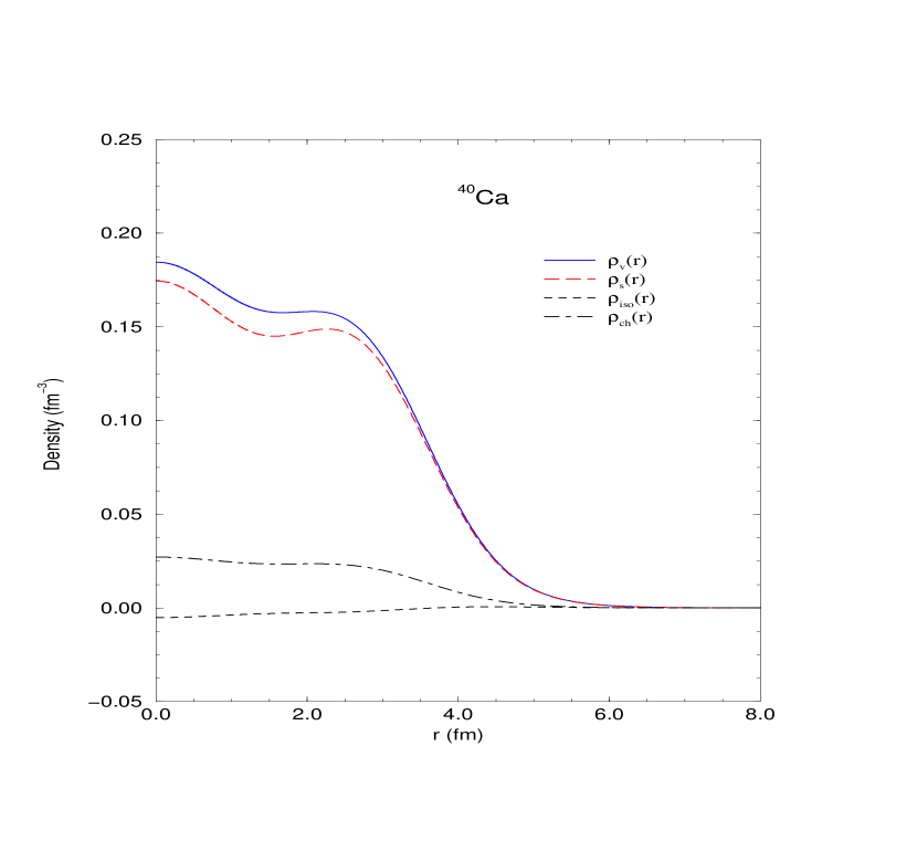
Figure 5: Various nuclear densities in ⁴⁰Ca: the vector (matter) density $\rho_{v}$, the scalar density $\rho_{s}$, the iso-vector density $\rho_{iso}$ (the difference between the proton and the neutron vector densities in the nucleus), and the charge density $\rho_{ch}$.

It includes the vector (matter) density $\rho_{v}$, the scalar density $\rho_{s}$, the iso-vector density $\rho_{iso}$ (the difference between the proton and the neutron vector densities in the nucleus), and the charge density $\rho_{ch}$. These densities generate the four different potentials in the nucleus: the $\sigma$ scalar potential $g_{s}\phi(r)$, the $\omega$ vector potential $g_{v}V(r)$, the $\rho$ vector potential $\frac{1}{2}g_{\rho}{b(r)}$, and the photon (electromagnetic) vector potential $eA(r)$ respectively. These potentials are shown in Figure 6.

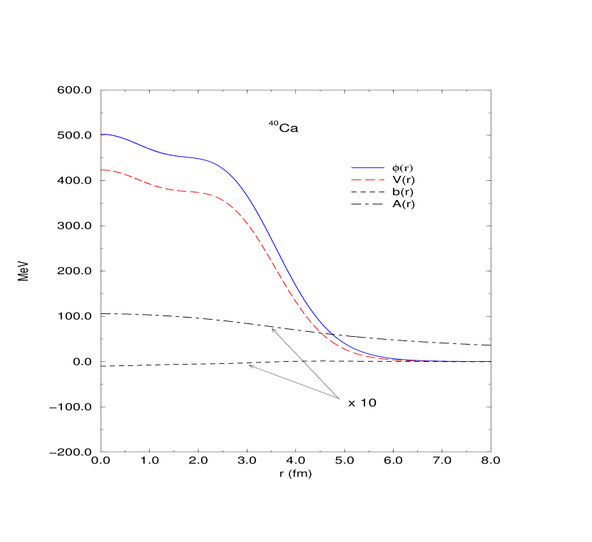
Figure 6: The different potentials in ⁴⁰Ca: the $\sigma$ scalar potential $g_{s}\phi(r)$, the $\omega$ vector potential $g_{v}V(r)$, the $\rho$ vector potential $\frac{1}{2}g_{\rho}b(r)$, and the photon (electromagnetic) vector potential $eA(r)$. The $b(r)$ and $A(r)$ potentials have been magnified by a factor of ten for better display.

In this figure, the $b(r)$ and $A(r)$ potentials have been magnified by a factor of ten for a better display.

Chapter 3 Theory of the Coherent Pseudoscalar Meson Photoproduction from Nuclei

In the four forthcoming chapters of this manuscript including this one, I will develop and discuss the first part of this doctoral study: the coherent pseudoscalar-meson photoproduction from nuclei. This process consists of a photon ($\gamma$-ray) incident on a nucleus. The photon interacts with the nucleus and as a result a pseudoscalar meson is produced (like $\pi$ or $\eta$ mesons) in addition to the recoil nucleus. In this way, we start the interaction with a photon and some nucleus, and end up with a meson and the same nucleus we started with. The process is labeled as “coherent” because all nucleons participate in the process leading to a coherent sum of these individual nucleon contributions.

1 Ingredients

The basic tenet of this theoretical study is the relativistic impulse approximation. It consists of the assumption that the process proceeds through the interaction of the incident photon with individual nucleons in the nucleus as opposed to interacting with the nucleus as a whole. Furthermore, the approximation assumes that the nature of the interaction between the photon and the bound nucleon is identical to the nature of the interaction between a photon and a free nucleon, apart from including the binding aspect of the nucleon. Figure 1 sketches this process within this approximation.

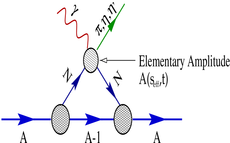
Figure 1: A schematic diagram for the coherent process within the framework of the impulse approximation. The incident photon is assumed to interact with individual nucleons in a nucleus ($A$) leading to the production of a pseudoscalar meson and the same, but now recoil, nucleus.

In our formalism we maintain the full relativistic structure whether in the elementary photoproduction process or in the nuclear structure. This approach forms a major departure from the traditional studies [8, 9, 10, 11, 12, 13] of this subject where one resorts to non-relativistic reduction of the elementary photoproduction amplitude and uses non-relativistic models for the nuclear structure to simplify the formalism. In this regard we use the Walecka model for the nuclear structure that we developed in Chapter 2.

Since mesons do in principle interact strongly with nucleons and nuclei, we have to account for the final-state interaction between the emitted meson and the recoil nucleus. This kind of final-state interaction is usually labeled as “distortion”, because instead of having a plane wave ($e^{-ik^{\prime}x}$) describing the meson wavefunction, we have a wave “distorted” from its plane-wave limit due to the presence of these interactions. We incorporate distortions through an optical potential formalism that will be the subject of the next chapter. To distinguish between two types of impulse approximation and to follow the conventional terminology in the literature, we label the relativistic impulse approximation with no final-state interactions as the relativistic plane-wave impulse approximation (RPWIA), while we refer to the approximation in the presence of distortions as the relativistic distorted-wave impulse approximation (RDWIA).

2 Differential Cross Section for the Coherent Process

The expression for the differential cross section has been derived using well established procedures for the case of two incoming particles and two outgoing ones [41]. Thus, we have the following form for the cross section in the center-of-momentum frame (c.m.)

$$\left({d\sigma\over d\Omega}\right)_{\rm c.m.}=\left({M_{\lower 1.0pt\hbox{$\scriptstyle T$}}\over 4\pi W}\right)^{2}\left({{k}^{\prime}_{\rm c.m.}\over{k}_{\rm c.m.}}\right){1\over 2}\sum_{\lambda}|{\mathcal{T}}_{\lower 2.0pt\hbox{$\scriptstyle\lambda$}}|^{2}\;,$$ (1)

where $M_{\lower 1.0pt\hbox{$\scriptstyle T$}}$ is the mass of the target nucleus, $W$ is the total energy in the c.m. frame, while ${k}_{\rm c.m.}\equiv|{\bf k}_{\rm c.m.}|$ and ${k}^{\prime}_{\rm c.m.}\equiv|{\bf k}^{\prime}_{\rm c.m.}|$ are the three-momenta of the photon and $\eta$-meson in the c.m. frame, respectively. This expression is independent of the mass of the produced meson and so it is applicable to the coherent photoproduction of any pseudoscalar meson. Restricting our formalism to coherent processes from nuclei with zero angular momentum and zero isospin ($J^{\pi}\!=\!0^{+};T\!=\!0$), the scattering matrix element $T_{\lower 2.0pt\hbox{$\scriptstyle\lambda$}}$ is given by

$${\mathcal{T}}_{\lower 2.0pt\hbox{$\scriptstyle\lambda$}}=\epsilon_{\mu}(\hat{\bf k},\lambda)\langle A(p^{\prime});\eta(k^{\prime})|J^{\mu}|A(p)\rangle\;,$$ (2)

This expression is nothing but the standard contraction in electrodynamics between the photon polarization $\epsilon_{\mu}(\hat{\bf k},\lambda)$ and the conserved electromagnetic current $\langle A(p^{\prime});\eta(k^{\prime})|J^{\mu}|A(p)\rangle$. Now using basic symmetry considerations that include parity and Lorentz covariance, we can write a model-independent form for the current matrix element as

$$\langle A(p^{\prime});\eta(k^{\prime})|J^{\mu}|A(p)\rangle=\varepsilon^{\mu\nu\alpha\beta}k_{\nu}k^{\prime}_{\alpha}p_{\beta}{1\over W}F_{0}(s,t)\;.$$ (3)

Here $p(p^{\prime}\!=\!p\!+\!k\!-\!k^{\prime})$ is the four momentum of the initial(final) nucleus and $\varepsilon^{\mu\nu\alpha\beta}$ is the relativistic Levi-Civita symbol ($\varepsilon^{0123}\equiv-1$). It is evident in this expression, and in fact a remarkable result, that the cross section cannot depend in this process on more than one Lorentz-invariant form factor $F_{0}(s,t)$, which is a function of the Mandelstam variables $s=(k+p)^{2}$ and $t=(k-k^{\prime})^{2}$. All dynamical information in this process must be contained in this form factor. Now substituting Equation 3 in Equation 1 and doing some algebraic manipulations we arrive at the following expression for the cross section

$$\left({d\sigma\over d\Omega}\right)_{\rm c.m.}=\left({M_{\lower 1.0pt\hbox{$\scriptstyle T$}}\over 4\pi W}\right)^{2}\left({k^{\prime}_{\rm c.m.}\over k_{\rm c.m.}}\right)\left({1\over 2}{k_{\rm c.m.}}^{2}{k^{\prime}_{\rm c.m.}}^{2}\sin^{2}\theta_{\rm c.m.}\right)|F_{0}(s,t)|^{2}\;,$$ (4)

where $\theta_{\rm c.m.}$ is the scattering angle (between ${\bf k}$ and ${\bf k}^{\prime}$) in the c.m. frame.

3 Determination of $F_{0}(s,t)$ in a Relativistic Impulse Approximation Approach

The most general expression for the scattering matrix element in the framework of the relativistic plane-wave impulse approximation can be written as a multiple integral in the following form

$$\sum_{\alpha}\int d^{4}x_{1}\ldots d^{4}x_{N}\;\overline{{\cal U}}_{\alpha}A^{\mu}J_{\mu}(x_{1},\ldots,x_{N}){\cal U}_{\alpha}\phi\;,$$ (5)

where ${\cal U}_{\alpha}$ is the single-particle Dirac spinor for the bound nucleon with a set of quantum numbers $\alpha$, $A^{\mu}$ is the photon wavefunction (field), and $\phi$ is the pseudoscalar meson wavefunction (field). The number $N$ of the independent variables to be integrated over depends on the nature of the effective field theory employed. In other words, it depends on the number of vertices in each Feynman diagram derived from this effective field theory. The sum $\sum_{\alpha}$ runs over all occupied states in the nucleus. It can be shown then that this expression can be reduced to the following form:

$$\sum_{\alpha}\int\;\frac{d^{3}p_{1}}{(2\pi)^{3}}\frac{d^{3}p_{2}}{(2\pi)^{3}}(2\pi)^{4}\delta^{4}(k+p_{1}-k^{\prime}-p_{2})\overline{{\cal U}}_{\alpha}{(\bf p_{1})}T(p_{1},p_{2},k,k^{\prime}){\cal U}_{\alpha}{(\bf p_{2})}\;,$$ (6)

where ${\cal U}_{\alpha}({\bf p})$ is the Dirac spinor in momentum space and where $T(p_{1},p_{2},k,k)\equiv\epsilon_{\mu}J^{\mu}(p_{1},p_{2},k,k^{\prime})$ is the scattering matrix introduced in Equation 2 of Chapter 1. The momenta $p_{1},p_{2},k,$ and $k^{\prime}$ are the four momenta of the struck nucleon, outgoing nucleon, incident photon, and emitted meson respectively. Note that here the struck and outgoing nucleons are bound and so they are not in a specific momentum state but have a momentum distribution.

The evaluation of this integral is involved. A great simplification ensues if one uses the factorization approximation (also called optimal approximation) of Gurvitz, Dedonder, and Amado [42]. The approximation is standard in this kind of study and consists of evaluating $T(p_{1},p_{2},k,k^{\prime})$ at certain optimal (effective) value of $p_{1}$ to enable us to “factorize” $T(p_{1},p_{2},k,k^{\prime})$ from the integral in such a way that minimizes any correction from the Fermi motion of the bound nucleon. More details on this optimal prescription will be presented in the next section. Thus, the approximation works best if $T(p_{1},p_{2},k,k^{\prime})$ is a slowly varying function of $p_{1}$. Using this approximation and replacing the $\delta$-function by its integral representation $\frac{1}{(2\pi)^{4}}\int d^{4}x\;e^{i(k+p_{1}-k^{\prime}-p_{2})\cdot x}$ one can arrive at the following form for the scattering matrix element

$$\sum_{\alpha}\delta(p_{1}^{0}+k^{0}-p_{2}^{0}-k^{\prime 0})\;\int d^{3}x\;e^{i{\bf q\cdot x}}\overline{{\cal U}}_{\alpha}{(\bf x)}T(p_{1},p_{2},k,k^{\prime}){\cal U}_{\alpha}{(\bf x)}\;,$$ (7)

where ${\bf q}={\bf k-k^{\prime}}$ is the momentum transfer. It is evident in this expression that the combination of the impulse and factorization approximations is effectively achieved by simply sandwiching the scattering matrix for the on-shell nucleons between bound-nucleon spinors instead of free spinors as is the case in the elementary process.

Now replacing $T$ by its expression in terms of the bilinear covariants (Chapter 1):

$$T[\gamma N\rightarrow PS\,meson\,N(Y)]=F^{\alpha\beta}_{T}\sigma_{\alpha\beta}+F_{P}i\gamma_{5}+F^{\alpha}_{A}\gamma_{\alpha}\gamma_{5}\;,$$ (8)

and taking advantage of basic definitions for the nuclear densities in the relativistic formalism (see Chapter 2) we arrive at

$$\delta(p_{1}^{0}+k^{0}-p_{2}^{0}-k^{\prime 0})\;\int d^{3}x\;e^{i{\bf q\cdot x}}\{F^{\alpha\beta}_{T}{\rho_{\alpha\beta}}_{\lower 3.0pt\hbox{$\scriptstyle T$}}({\bf x})+F_{P}i{\rho}_{\lower 3.0pt\hbox{$\scriptstyle PS$}}({\bf x})+F^{\alpha}_{A}{\rho_{\alpha}}_{\lower 3.0pt\hbox{$\scriptstyle AV$}}({\bf x)}\}\;.$$ (9)

Thus the coherent process probes three nuclear densities in the nucleus: the tensor (T), pseudoscalar (PS), and axial-vector (AV) densities. However, as has been indicated in Chapter 2, the pseudoscalar and axial-vector densities vanish for ($J^{\pi}\!=\!0^{+};T\!=\!0$) nuclei. In fact even all components of the tensor density vanish except the three ${\rho_{0i}}_{\lower 3.0pt\hbox{$\scriptstyle T$}}$ where $i=1,2,3$. Substituting the expressions for $F^{\alpha\beta}_{T}$ and ${\rho_{\alpha\beta}}_{\lower 3.0pt\hbox{$\scriptstyle T$}}({\bf x})$ and carrying out some algebraic manipulations we arrive at a remarkably simple expression for the the coherent-process scattering matrix element in the c.m. frame:

$$\delta(p_{1}^{0}+k^{0}-p_{2}^{0}-k^{\prime 0})\,iA_{1}(s,t)\frac{\rho_{\lower 3.0pt\hbox{$\scriptstyle T$}}(q)}{q}\Big{\{}kk^{\prime}{\bf\hat{k^{\prime}}}\cdot\left[{\bf\hat{k}}\times\mbox{\boldmath$\epsilon$ \unboldmath}(\hat{\bf k},\lambda)\right]\Big{\}}\;,$$ (10)

where

$$\rho_{\lower 3.0pt\hbox{$\scriptstyle T$}}(q)=4\pi\int_{0}^{\infty}dr\,r^{2}j_{\lower 2.0pt\hbox{$\scriptstyle 1$}}(qr)\rho_{\lower 3.0pt\hbox{$\scriptstyle T$}}(r)\;.$$ (11)

Taking this form, we can then find the expression for the differential cross section in the relativistic plane-wave-impulse-approximation approach. By comparing this expression to the model-independent one given by Equation 4, we can extract the value of the Lorentz-invariant form factor $F_{0}(s,t)$ to be

$$F_{0}^{\scriptscriptstyle PW}(s,t)=iA_{1}(s,t)\frac{\rho_{\lower 3.0pt\hbox{$\scriptstyle T$}}(q)}{q}\;.$$ (12)

It is important to stress here that the analysis I sketched here is valid only in the plane-wave limit where no distortions for the emitted meson have been incorporated. Including these distortions spoils this simple and elegant result. This will be the subject of the next chapter.

4 More on the Factorization Approximation: the Optimal Prescription

In the previous section I have hinted at the basic idea of the factorization approximation. What remains is to find the optimal value for ${\bf p}_{1}$ which is determined using what is called the “optimal prescription” [42]. Since in Equation 10 all kinematic quantities are fixed except for $s$ ($t$ and $q$ are determined from the measured ${\bf k}$ and ${\bf k^{\prime}}$), we are trying effectively to find the optimal value for $s$ (call it $\tilde{s}$) for the coherent process.

The optimal value of ${\bf p}_{1}$ is determined by the principle of “democratic” sharing of momentum expressed as:

$$\frac{{\bf p_{1}}+{\bf p_{2}}}{2}={\bf P}_{avg}\;,$$ (13)

where ${\bf P}_{avg}$ is the average momentum carried by a spectator nucleon during the collision. Since only one nucleon participates in the interaction in the impulse-approximation picture, ${\bf P}_{avg}$ is the average momentum of the other nucleons in the nucleus. Using this condition and the conservation of momentum during the collision

$${\bf P_{A}}+{\bf k}={\bf P^{\prime}_{A}}+{\bf k^{\prime}}\;,$$ (14)

where ${\bf P_{A}}$ (${\bf P^{\prime}_{A}}$) is the momentum of the nucleus before (after) the collision, as well as the conservation of momentum at the interaction vertex (see Figure 1)

$${\bf p_{1}}+{\bf k}={\bf p_{2}}+{\bf k^{\prime}}\;,$$ (15)

one can show that the effective momentum of the struck nucleon is given by (in the c.m frame)

$${\bf p_{1}}=-\frac{A+1}{2A}{\bf k}_{cm}+\frac{A-1}{2A}{\bf k^{\prime}}_{cm}\;,$$ (16)

while the effective momentum of the outgoing nucleon is expressed as

$${\bf p_{2}}=\frac{A-1}{2A}{\bf k}_{cm}-\frac{A+1}{2A}{\bf k^{\prime}}_{cm}\;.$$ (17)

As a result, it is straightforward to find the optimal value $\tilde{s}$ as

$${\tilde{s}}={M^{2}}_{N}+2k_{cm}(E_{1}-p_{1}cos\theta_{1})\;,$$ (18)

where

$$E_{1} = ({M^{2}}_{N}+\alpha^{2}{k}_{cm}^{2}+\alpha^{\prime 2}{k^{\prime}}_{cm}^{2}-2\alpha\alpha^{\prime}k_{cm}{k^{\prime}}_{cm}cos\theta_{cm})^{\frac{1}{2}}\;,$$ (19)

$$p_{1}cos\theta_{1} = -\alpha{k}_{cm}+\alpha^{\prime}{k^{\prime}}_{cm}cos\theta_{cm}\;,$$

$$\alpha \equiv \frac{A+1}{2A}\;,$$

$$\alpha^{\prime} \equiv \frac{A-1}{2A}\;,$$

where $M_{N}$ is the mass of the nucleon, and ${p_{1}}$, ${k}_{cm}$, and ${k}^{\prime}_{cm}$ are the three-momenta of the bound nucleon, incident photon, and emitted meson respectively. Moreover, $\theta_{1}$ is the angle between ${\bf k}$ and ${\bf p_{1}}$, and $\theta_{cm}$ is the scattering angle between ${\bf k}$ and ${\bf k^{\prime}}$.

5 Off-Shell Ambiguity

The study of the coherent reaction represents a challenging theoretical task due to the lack of a detailed microscopic model of the process. Indeed, most of the models used to date rely on the impulse approximation assumption that the elementary amplitude remains unchanged as the process is embedded in the nuclear medium. Yet, even a detailed knowledge of the elementary amplitude does not guarantee a good understanding of the coherent process. The main difficulty stems from the fact that there are, literally, an infinite number of equivalent on-shell representations of the elementary amplitude. These different representations—although equivalent on-shell—can give very different results when evaluated off-shell. We will present in this section an example of this ambiguity and later on in our discussion of the results (Chapter 5) we will show how two equivalent parameterizations on-shell can give results that are an order of magnitude apart for off-shell spinors. Of course, this uncertainty is present in many other kinds of nuclear reactions, not just in the coherent photoproduction process. Yet, this off-shell ambiguity comprises one of the biggest, if not the biggest, hurdle in understanding the coherent photoproduction of pseudoscalar mesons.

In Chapter 1, I have included the standard form for the amplitude of the elementary process $\gamma N\rightarrow PS\,meson\,N(Y)$ as

$$T[\gamma N\rightarrow PS\,meson\,N(Y)]=\sum_{i=1}^{4}A_{i}(s,t)M_{i}\,,$$ (20)

where the invariant matrices have the form

$$M_{1} = -\gamma^{5}\hbox to0.0pt{/\hss}{\varepsilon}\hbox to0.0pt{/\hss}k\,,$$

$$M_{2} = 2\gamma^{5}[(\varepsilon\cdot p_{1})(k\cdot p_{2})-(\varepsilon\cdot p_{2})(k\cdot p_{1})]\,,$$

$$M_{3} = \gamma^{5}[\hbox to0.0pt{/\hss}{\varepsilon}((k\cdot p_{1})-\hbox to0.0pt{/\hss}k(\varepsilon\cdot p_{1})]\,,$$

$$M_{4} = \gamma^{5}[\hbox to0.0pt{/\hss}{\varepsilon}((k\cdot p_{2})-\hbox to0.0pt{/\hss}k(\varepsilon\cdot p_{2})]\;.$$ (21)

I indicated then that this form although complete and standard, is not unique. Many other choices—all of them equivalent on shell—are possible. Indeed, we could have used the relation—valid only on the mass shell,

$${M}_{1} = -\gamma^{5}\hbox to0.0pt{/\hss}{\epsilon}\;\hbox to0.0pt{/\hss}{k}={1\over 2}\varepsilon^{\mu\nu\alpha\beta}\,\epsilon_{\mu}\,k_{\nu}\sigma_{\alpha\beta}={i\over 2}\varepsilon^{\mu\nu\alpha\beta}\,\epsilon_{\mu}\,k_{\nu}\,{q_{\alpha}\over M_{N}}\gamma_{\beta}$$ (22)

$$- {1\over 2M_{N}}\gamma^{5}\Big{[}\hbox to0.0pt{/\hss}{\epsilon}\,(k\cdot p)-\hbox to0.0pt{/\hss}{k}(\epsilon\cdot p)\Big{]}-{1\over 2M_{N}}\gamma^{5}\Big{[}\hbox to0.0pt{/\hss}{\epsilon}\,(k\cdot p^{\prime})-\hbox to0.0pt{/\hss}{k}(\epsilon\cdot p^{\prime})\Big{]}\;,$$

to obtain the following representation of the elementary amplitude:

$$T[\gamma N\rightarrow PS\,meson\,N(Y)]=\sum_{i=1}^{4}B_{i}(s,t){N}_{i}\;,$$ (23)

where the new invariant amplitudes and Lorentz structures are now defined as:

$$B_{1} = A_{1}\;;\qquad\phantom{-,A_{1}/2M}\;\;N_{1}={i\over 2}\varepsilon^{\mu\nu\alpha\beta}\,\epsilon_{\mu}\,k_{\nu}\,{q_{\alpha}\over M_{N}}\gamma_{\beta}\;,$$ (24)

$$B_{2} = A_{2}\;;\qquad\phantom{-,A_{1}/2M_{N}}N_{2}=M_{2}=2\gamma^{5}\Big{[}(\epsilon\cdot p)(k\cdot p^{\prime})-(\epsilon\cdot p^{\prime})(k\cdot p)\Big{]}\;,$$ (25)

$$B_{3} = A_{3}-A_{1}/2M_{N}\;;\qquad N_{3}=M_{3}=\gamma^{5}\Big{[}\hbox to0.0pt{/\hss}{\epsilon}\,(k\cdot p)-\hbox to0.0pt{/\hss}{k}(\epsilon\cdot p)\Big{]}\;,$$ (26)

$$B_{4} = A_{4}-A_{1}/2M_{N}\;;\qquad N_{4}=M_{4}=\gamma^{5}\Big{[}\hbox to0.0pt{/\hss}{\epsilon}\,(k\cdot p^{\prime})-\hbox to0.0pt{/\hss}{k}(\epsilon\cdot p^{\prime})\Big{]}\;.$$ (27)

Although clearly different, Equations 20 and 23 are totally equivalent on-shell: no observable measured in the elementary process could distinguish between these two forms. We could go on. In fact, it is well known that a pseudoscalar and a pseudovector representation are equivalent on shell. That is, we could substitute the pseudoscalar vertex in $N_{2}$ and $M_{2}$ by a pseudovector one:

$$\gamma^{5}={\hbox to0.0pt{/\hss}{\!q}\over 2M_{N}}\gamma^{5}\;.$$ (28)

The possibilities seem endless.

Given the fact that there are many—indeed infinite—equivalent parameterizations of the elementary amplitude on-shell, it becomes ambiguous on how to take the amplitude off the mass shell. The question that arises here: are these equivalent representations on-shell, still equivalent when we consider bound nucleons; nucleons that are off their mass shell? The answer is negative. In this work we have examined this off-shell ambiguity by studying the coherent process using the “tensor” parameterization, as in Equation 20, and the “vector” parameterization, as in Equation 23. Denoting these parameterizations as tensor and vector originates from the fact that for the coherent process from spherical nuclei (such as the ones considered here) the respective cross sections become sensitive to only the tensor and vector (matter) densities, respectively. Indeed, we have seen in the previous section that the standard form for the amplitude resulted in the process probing the tensor density of the nucleus.

It is important to note here that the vector and tensor densities are fundamentally different quantities and that this off-shell ambiguity is a direct consequence of using the fully relativistic formalism. Had we elected to use non-relativistic formalisms [8, 9, 10, 11, 12, 13], we would have found that the process is probing the vector (matter) density and that there is no off-shell ambiguity. This is, however, due to the limitations of the non-relativistic nuclear structure formalism which cannot produce more than one nuclear density due to the arbitrary neglect of any medium modifications to the ratio of lower-to-upper components of the Dirac spinors as a result of using the free-space relation to relate these components to each other.

Since the substance of the difference between the tensor and vector parameterizations lies in the use of the tensor as opposed to the vector density of the nucleus, it is instructive to find the relationship between these two quantities. This can be most easily seen by assuming the free-space relation between the upper and lower components of the Dirac spinors. In this case the tensor density can be written in terms of the vector density as

$$\rho_{\lower 3.0pt\hbox{$\scriptstyle T$}}(q)=-{q\over 2M_{N}}\rho_{\lower 3.0pt\hbox{$\scriptstyle V$}}(q)+\sum_{\alpha}^{\rm{occ}}{{\kappa+1}\over M_{N}}\int_{0}^{\infty}dr{{g^{2}_{\alpha}(r)}\over r^{2}}j_{1}(qr)\;,$$ (29)

where $\kappa$ is the generalized relativistic angular momentum (see Chapter 2), ${g_{\alpha}(r)}$ is the upper component of the Dirac spinor, and $j_{1}(qr)$ is the Bessel function of order one. The second term in the above expression is negligible for closed-shell (spin-saturated) nuclei; this term is proportional to the difference between the square of the wavefunctions of spin-orbit partners (such as $p^{3/2}$ and $p^{1/2}$ orbitals) which is very small even in the Walecka model. Hence, for closed shell nuclei—and adopting a free-space relation—the tensor density becomes proportional to the vector density. Thus we have produced the non-relativistic limit of the tensor density. However, for open-shell nuclei such as ¹²C, the second term in Equation 29 is no longer negligible and leads to an additional enhancement of the tensor density—above and beyond the one obtained from the the dynamic enhancement of the lower component of the Dirac spinor. We label this additional enhancement of the cross section as “open-shell effect” to distinguish it from the dynamic enhancement.

To a provide a feeling for the nature of the nuclear tensor density ($\rho_{T}$) and its dependence on the nucleus radius, Figure 2 displays the proton and neutron tensor densities in

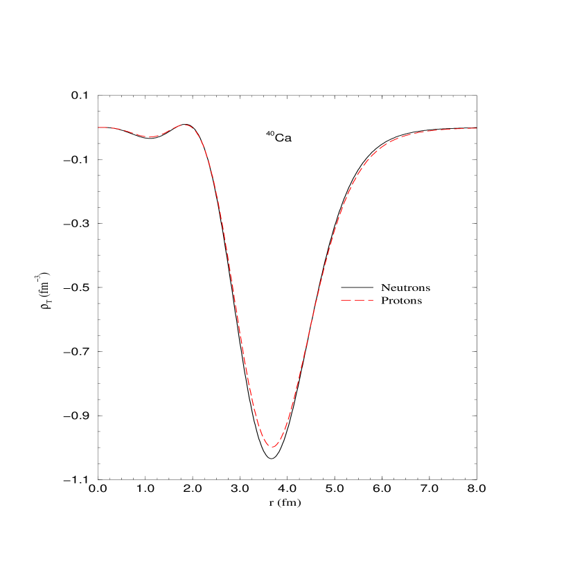
Figure 2: The proton and neutron tensor densities [$\rho_{T}(r)$] in ⁴⁰Ca as calculated using the QHD-II model for the nuclear structure.

⁴⁰Ca. As evident in this figure, the tensor density has a different behavior compared to the vector and scalar densities; it is appreciable only at the surface of the nucleus and vanishing elsewhere (compare to Figure 5). The densities in the figure are calculated using the QHD-II model for the nuclear structure (Chapter 2). QHD-I evaluation gives identical results.

6 Inclusion of Isospin

Recall that the elementary process parameterization contains four amplitudes: $\{A_{1},A_{2},A_{3},A_{4}\}$. These have different values depending on the kind of nucleon target: a proton (p) or a neutron (n). Since nuclei include both of these nucleons, we have to modify our formalism to incorporate the isospin aspect of the problem. Thus, the $T$ matrix is modified as

$$T\Longrightarrow T_{p}\frac{1}{2}(1+\tau_{z})+T_{n}\frac{1}{2}(1-\tau_{z})\;.$$ (30)

Now substituting this form in our formalism for the coherent process results in the scattering matrix element depending on two combinations of the $A_{1}$ amplitude for the proton (${A_{1}}_{p}$) and the neutron (${A_{1}}_{n}$) : $A_{s}$ and $A_{v}$ as

$$T_{\mbox{coherent}}\sim A_{s}+A_{v}\tau_{z}\;,$$ (31)

where $A_{s}=\frac{1}{2}({A_{1}}_{p}+{A_{1}}_{n})$ and $A_{v}=\frac{1}{2}({A_{1}}_{p}-{A_{1}}_{n})$. Hence, it is clear that the $A_{s}$ part carries the isoscalar component of the matrix element while the $A_{v}$ part includes the isovector component. We arrive then at an expression for the matrix element (in the tensor parameterization) of the form

$$T_{\mbox{coherent}}\sim A_{s}{\rho_{T}}_{s}+A_{v}{\rho_{T}}_{v}\;,$$ (32)

where ${\rho_{T}}_{s}={\rho_{T}}_{p}+{\rho_{T}}_{n}$ and ${\rho_{T}}_{v}={\rho_{T}}_{p}-{\rho_{T}}_{n}$. That is the matrix element depends on two combinations of the proton and neutron tensor densities. Analogous expressions hold if we would have used the vector parameterization.

For the nuclei that we studied in this work, the proton and neutron numbers are equal. Therefore, ${\rho_{T}}_{p}\approx{\rho_{T}}_{n}$ and so $\rho_{v}\rightarrow 0$. That is the isovector component vanishes. Note that although $N_{p}=N_{n}$, for these nuclei, the cancellation between ${\rho_{T}}_{p}$ and ${\rho_{T}}_{n}$ is not perfect because of isospin symmetry violation in the Hamiltonian of the nucleus due mainly to the Coulomb repulsion of the protons. It is found however that this cancellation is almost exact and affect minimally the coherent process (see Chapter 5).

Chapter 4 Distortions and the Coherent Process

In the previous chapter, I have depicted the basic formalism for the coherent process in the limit of no final-state interactions between the emitted meson and the recoil nucleus. The expressions that we reached are elegant and transparent, but this beauty cannot survive the hammering of distortions. In this chapter, I will outline the modifications to this formalism in the presence of distortions. In the first section I will describe the basic mechanisms behind the meson-nucleus interaction while in the second one I will lay out the changes to the coherent-process formalism.

1 Optical Potential Formalism

Mesonic distortions play a critical role in all studies involving meson-nucleus interactions. These distortions are strong, and thus modify significantly any process relative to its naive plane-wave limit. Indeed, it has been shown in earlier studies of the coherent processes—and verified experimentally [11]—that there is a large modification of the plane-wave cross section once distortions are included. Fortunately, the meson-nucleus interaction is short range and present only in the close vicinity of the collision. The long-range Coulomb distortions do not play a role here since the emitted meson must be electrically neutral due to charge conservation. Because of the importance of mesonic distortions, any realistic study of the coherent reaction must invoke them from the outset. However, since a detailed microscopic model for distortions has yet to be developed, I have resorted to a semi-phenomenological method: optical-potential formalism.

1 Equation of Motion for the Meson Field

In this section, the equation of motion for the meson will be discussed. Since the mass of the emitted meson is comparable to the momentum carried by this particle, the meson must be treated relativistically. On the other hand, the nucleus has a much larger mass compared to its momentum and thus can be treated non-relativistically at least in the low-energy scattering processes.

There are at least three approaches to write the effective equation of motion for the meson-nucleus interaction. The simplest one is to consider the nucleus as a static source of potential in which the meson travels through. Consequently, we have a one-body Klein-Gordon equation of the form:

$$\left(D_{\mu}D^{\mu}+m^{2}\right)\phi=0\;,$$ (1)

where $D_{\mu}=i\partial_{\mu}-V_{\mu}(x)$, $V_{\mu}$ is the interaction potential, and $m$ is the mass of the meson [11, 43].

Another approach is to write a “relativized” Schrodinger-like equation for the system as

$$\left[(-{\nabla^{2}}_{x}+m^{2})^{\frac{1}{2}}+M_{A}+\frac{-{\nabla^{2}}_{x^{\prime}}}{2M_{A}}+V({\bf x,x^{\prime}})\right]\psi=i\partial_{t}\psi\;,$$ (2)

where in this equation $\nabla^{2}=\partial_{i}\partial^{i}$, $x$ denotes the meson coordinates while $x^{\prime}$ denotes the nucleus coordinates, $M_{A}$ is the nucleus mass, $V({\bf x,x^{\prime}})$ is the interaction potential, and $\psi$ is the meson-nucleus system wavefunction [18, 44]. It is clear in the equation that the kinetic energy term for the meson has been relativized $(-{\nabla^{2}}_{x}+m^{2})^{\frac{1}{2}}$, while the one for the nucleus has its non-relativistic form ($\frac{-{\nabla^{2}}_{x}^{\prime}}{2M_{A}}$).

A third approach is to write a Klein-Gordon-like equation for the system as [18]

$$\left(-{\nabla^{2}}_{x}+m^{2}\right)\psi=\left(i\partial_{t}-V({\bf x,x^{\prime}})-M_{A}-\frac{-{\nabla^{2}}_{x^{\prime}}}{2M_{A}}\right)^{2}\psi\;.$$ (3)

Goldberger and Watson [44] have shown that the second and third of these approaches (Equations 2 and 3) are equivalent for certain class of potentials.

Starting with Equation 3, one can arrive at an effective one-body equation for the meson field by absorbing the nucleus degrees of freedom and using several assumptions about the nature of the interaction, to yield the eigenvalue equation:

$$\left[{\nabla^{2}}+{\bf k}^{2}-2\omega U(r)\right]\phi=0\;,$$ (4)

where ${\bf k}$ is the meson asymptotic momentum in the center-of-momentum frame (c.m.), and $2\omega U(r)$ is the effective potential for this one-body equation. This potential is an involved nonlocal function of the potential $V$ and several kinematic variables in the problem [18]. We adopt this third approach for our studies.

The potential $2\omega U(r)$ is independent of the angular coordinates $(\Phi,\theta)$ and thus we can separate the angular parts from the radial part in the equation. The angular parts reduce to the orbital-angular-momentum equations which have the spherical harmonics as their solutions, while the radial part reduces to the following equation:

$$\left[\frac{d^{2}}{dr^{2}}-\frac{l(l+1)}{r^{2}}+{\bf k}^{2}\right]u_{nl}(r)=r2\omega U(r)\,\left[\frac{u_{nl}(r)}{r}\right]\;,$$ (5)

where $l$ is the orbital angular momentum quantum number, $n$ is the energy quantum number, and $u_{nl}(r)$ is the radial part for a specific $l$-partial wave (angular-momentum channel) of the meson wavefunction. Consequently, the meson wavefunction is given by the expansion

$$\phi_{\mathbf{k}^{\prime}}=\sum_{l,m}4\pi(i)^{l}\;\frac{u_{nl}(r)}{r}\;Y_{lm}(\hat{\mathbf{r}})\;Y_{lm}^{*}(\hat{\mathbf{k^{\prime}}})\;,$$ (6)

where $m$ is the quantum number for the z-axis projection of the angular momentum and $Y_{lm}$ is the spherical harmonic with $l$ and $m$ orders.

2 Meson-Nucleus Optical Potential Form

The potential $2\omega U(r)$ for the kind of applications that we are considering here has the formal form:

$$2\omega U(r)=f_{1}(r)+\nabla^{2}f_{2}(r)+\mbox{\boldmath${\nabla}$ \unboldmath}\cdot f_{3}(r)\mbox{\boldmath${\nabla}$ \unboldmath}\;,$$ (7)

where $f_{i}(r)$ are some functions. Such form can also be rewritten as

$$2\omega U(r)=f_{1}(r)+\frac{2}{r}\frac{df_{2}(r)}{dr}+\frac{d^{2}f_{2}(r)}{dr^{2}}+f_{3}(r)\nabla^{2}+\frac{df_{3}(r)}{dr}\frac{d}{dr}\;.$$ (8)

We have studied in this work the coherent process for the production of $\eta$ and $\pi$ mesons. Thus, I will outline here two kinds of optical potentials: the $\eta$-nucleus and the $\pi$-nucleus optical potentials.

Eta-Nucleus Optical Potential

We have been very fortunate to find a simple and local form for the $\eta$-nucleus optical potential in the literature; a fortune that we lacked in the case of the $\pi$-nucleus potential. This simplicity is due the fact that the $\pi$-nucleus interaction is far stronger and sophisticated than the $\eta$-nucleus interaction. For the $\eta$-nucleus interaction in the low energy regime of our interest, $s$-wave components dominates, and $p$-wave and $d$-wave contributions are very small. This in turn is a result of the fact that the $\eta$ ($0$-isospin) can couple only to $\frac{1}{2}$-isospin nucleon resonances like the $S_{11}$, and cannot couple to the $\Delta$-resonance which has an isospin of $\frac{3}{2}$. Consequently, there are only few resonances that the $\eta$ can couple to leading to a simple form for the $\eta$-nucleus interaction. This situation is in sharp contrast to the $\pi$-nucleus interaction presented in the next section where the pion can couple strongly to several nucleon resonances.

The optical potential expression is constructed from the scattering amplitude of the process $\eta N\rightarrow\eta N$ to fit a simple $t\rho$ form [10] as following :

$$2\omega U(r)=-b\rho_{\lower 3.0pt\hbox{$\scriptstyle V$}}(r)\;.$$ (9)

Here $\rho_{\lower 3.0pt\hbox{$\scriptstyle V$}}(r)$ is the vector density of the nucleus and and $b$ is a complex two-body ($\eta N$) parameter that is given by the following:

$$b(p_{\rm lab}) \equiv (\alpha+\beta p_{\rm lab}+\gamma p_{\rm lab}^{2})^{-1}\;,$$ (10)

$$\alpha = (+0.136,-0.052)\,{\rm fm}^{-1}\;,$$ (11)

$$\beta = (+0.035,-0.072)\;,$$ (12)

$$\gamma = (-0.061,+0.009)\,{\rm fm}\;.$$ (13)

Having this simple form for the potential, one can solve numerically the radial part of the Klein-Gordon equation 5 for each partial wave to obtain the full outgoing $\eta$-meson wavefunction (Equation 6).

Pion-Nucleus Optical Potential

Constructing the $\pi$-nucleus optical potential proved to be a difficult task. Admittedly, there is a lot of work in the literature that covers this issue. Nevertheless, most studies concentrated on the low energy optical potential and I was not able to find any work that derives the optical potential in the $\Delta$-resonance region. Consequently, J. Carr and I extended earlier studies [18] on the low-energy $\pi$-nucleus optical potential to higher energies so that they cover the $\Delta$ resonance region [5]. A pleasant by-product emerged from our study: we were able to update earlier studies with our newly extracted optical potential parameters from recent state-of-the-art experimental measurements [45]. In this regard, this project can serve as a current comparative view of earlier attempts to extract these parameters. Furthermore, we make no recourse to nonrelativistic approximations (as opposed to the earlier low-energy treatments), and include the full relativistic nucleus recoil.

The derivation of the optical potential form is a challenging endeavor for the following reasons: first, the $\pi$-nucleus interaction is very strong which renders the fine details in the potential significant. Second, the first-order impulse-approximation form of the potential is not adequate as one has to incorporate many corrections stemming from the many-body nature of the interaction like multiple scattering and pion absorption. Indeed, pion absorption is crucial in the $\Delta$ resonance. Finally, the nature of the potential is complicated as it involves local and nonlocal terms. These complications arise in fact from the essence of the fundamental process that drives the interaction in this energy regime: the $\Delta$ resonance formation. Since the procedures for this derivation are very involved, for the purpose of this manuscript, I will give only an overview of the derivation as well as the final form of the optical potential.

The $\pi$-nucleus optical potential is derived using a semi-phenomenological formalism that originates in the $\pi-N$ interaction scattering amplitude. This amplitude is given by [18]

$$f(\pi N\rightarrow\pi N)=b_{0}+b_{1}\;{\bf t}\cdot\mbox{\boldmath$\tau$ \unboldmath}+(c_{0}+c_{1}\;{\bf t}\cdot\mbox{\boldmath$\tau$\unboldmath})\;{\bf k}.{\bf k}^{\prime}\;,$$ (14)

where ${\bf t}$ and $\tau$ are the pion and nucleon isospin operators, ${\bf k}$ and ${\bf k}^{\prime}$ are the incoming and outgoing pion momenta, $b_{0}$ and $b_{1}$ are the s-wave parameters and $c_{0}$ and $c_{1}$ are the p-wave parameters. In this form the small spin-dependent term has been neglected. The s- and p-wave parameters are determined from the phase shifts. In earlier treatments [18], these parameters were determined initially from a phase shift analysis performed by Rowe, Salomon, and Landau [46]. The parameters then were slightly modified to obtain the best fit for the $\pi$-nucleus scattering and pionic atom data. Our treatment differs from the previous studies in two aspects: first, we determine them from the state-of-the-art experimental measurements and phase shift analysis (SP98) of Arndt, Strakovsky, Workman, and Pavan from the Virginia Tech SAID program [45]. Second, we keep these parameters intact by not attempting to change them to fit any specific data. In doing so we have kept the theoretical basis for the optical potential unblemished. Nonetheless, the parameters determined by the two methods match nicely in the low-energy limit.

After adopting the $\pi-N$ scattering amplitude of Equation 14 in the center-of-momentum frame (c.m.), the first step in the derivation is to transform the scattering amplitude to the $\pi$-nucleus c.m. frame. This is done using the relativistic potential theory of Kerman, McManus, and Thaler [47]. The kinematic arguments of the scattering amplitude are then expressed in terms of the appropriate kinematic quantities in the $\pi$-nucleus c.m. frame using what is referred to as the angle transformation. In this manner, we would have achieved most of the first class of modifications to the scattering amplitude: kinematic corrections.

By invoking the impulse approximation, the resultant form for the amplitude is then sandwiched between bound-nucleon states and the expression is summed over all occupied states of the nucleus. Hence, one obtains the $\pi$-nucleus interaction amplitude in momentum space. Now taking the Fourier transform, we obtain an expression for the optical potential form.

This impulse-approximation form still lacks the second class of modifications: physical corrections resulting from many-body processes. These corrections modify the scattering amplitude parameters like $b_{0}$ and $c_{0}$ and add new terms to the optical potential. The first of these corrections are the multiple scattering ones. It has been found that the second-order corrections for the $s$-wave terms as well as higher order corrections for $p$-wave terms, are necessary. Therefore, the multiple scattering series for the p-wave is summed partially to all orders. This introduces the Ericson-Ericson effect [48] which is analogous to the Lorentz-Lorenz effect in electrodynamics [49]. This effect adds a nonlocal term to the potential of the form $\mbox{\boldmath${\nabla}$ \unboldmath}\cdot f(r)\mbox{\boldmath${\nabla}$ \unboldmath}$. The Ericson-Ericson term is further modified to account for short-range correlations between nucleons.

A second physical correction is the absorption correction. This one gives the potential its name as an “optical” potential since it implies the existence of an imaginary part in the potential. There are two types of absorption. The first one arises from the fact that there are many open inelastic channels in the $\pi$-nucleus interaction like nucleon knock-out. Accordingly, part of the incoming flux is absorbed by these processes leading to an imaginary part in the potential. This kind of absorption is naturally included in the impulse-approximation form for the potential. The second type of absorption arises from many-body mechanisms like the two-nucleon absorption where the pion is scattered from one nucleon but then absorbed by another. This is in fact the dominant many-body absorption mechanism. Another less important absorption mechanism, is the quasi-elastic charge exchange process. All of these many-body absorption mechanisms are referred to as true absorption to distinguish them from the inelastic (type one) absorptions. Ironically, the $\Delta$-resonance formation that drives strongly the elementary process $\pi N\rightarrow\pi N$, dampens it in the nucleus through the absorption mechanisms.

Another alteration to the potential is the Pauli correction. Due to the Pauli principle, the number of available final states for the struck nucleon in the nucleus is reduced by Pauli blocking leading to this kind of correction. Another correction is the Coulomb one originating from the fact that the incoming charged pion (in $\pi$-nucleus scattering) is accelerated or decelerated depending on its charge, by the Coulomb field of the nucleus before interacting with the nucleus through the strong interaction. This correction is of no impact in our study as we are considering coherent processes where the emitted pion is always neutral. Finally, it is noteworthy to mention that there are also other kinematic corrections stemming from transformation properties of the many-body subsystems like the $\pi-2N$ subsystem in the $\pi-2N$ interaction mechanisms.

After implementing these corrections to the impulse-approximation expression, we arrive at a pion-nucleus optical potential—applicable from threshold up to the delta-resonance region—of the form:

$$2\omega U \!=\! \!-4\pi\Big{[}p_{1}b(r)\!+\!p_{2}B(r)\!-\!\mbox{\boldmath${\nabla}$ \unboldmath}Q(r)\cdot\mbox{\boldmath${\nabla}$ \unboldmath}$$

$$\!-\!\;\frac{1}{4}p_{1}u_{1}{\nabla}^{2}c(r)\!-\!\frac{1}{4}p_{2}u_{2}{\nabla}^{2}C(r)\!+\!p_{1}y_{1}\widetilde{K}(r)\Big{]}\;,$$

where

$$b(r) = \bar{b}_{0}\rho(r)-\epsilon_{\pi}{b_{1}}{\delta}\rho(r)\;,$$ (16)

$$B(r) = {B_{0}}\rho^{2}(r)-\epsilon_{\pi}{B_{1}}\rho(r)\delta\rho(r)\;,$$ (17)

$$c(r) = c_{0}\rho(r)-\epsilon_{\pi}{c_{1}}{\delta}\rho(r)\;,$$ (18)

$$C(r) = C_{0}\rho^{2}(r)-\epsilon_{\pi}{C_{1}}\rho(r){\delta}\rho(r)\;,$$ (19)

$$Q(r) = \frac{L(r)}{1+\frac{4\pi}{3}\lambda L(r)}+p_{1}x_{1}\acute{c}\rho(r)\;,$$ (20)

$$L(r) = p_{1}x_{1}c(r)+p_{2}x_{2}C(r)\;,$$ (21)

$$\widetilde{K}(r) = \frac{3}{5}\left({\frac{3\pi^{2}}{2}}\right)^{2/3}c_{0}\rho^{5/3}(r)\;,$$ (22)

and with

$$\bar{b}_{0} = {b_{0}}-p_{1}\frac{A-1}{A}(b^{2}_{0}+2b^{2}_{1})I\;,$$ (23)

$$\acute{c} = p_{1}x_{1}\frac{1}{3}k^{2}_{o}(c^{2}_{0}+2c^{2}_{1})I\;.$$ (24)

In the above expressions, the set {$p_{1},u_{1},x_{1},$ and $y_{1}$} represents various kinematic factors in the effective $\pi-N$ system (pion-nucleon mechanisms), and the set {$p_{2},u_{2},$ and $x_{2}$} represents the corresponding kinematic factors in the $\pi\!-\!2N$ system (pion-two-nucleon mechanisms). The set of parameters {$b_{0},b_{1},c_{0},$ and $c_{1}$} originates from the $\pi N\!\rightarrow\!\pi N$ elementary amplitudes while all other parameters–excluding the kinematic factors–have their origin in the second and higher order corrections to the optical potential. Nuclear effects enter in the optical potential through the nuclear density $\rho(r)$, and through the neutron-proton density difference (isovector density) $\delta\rho(r)$. Moreover, $A$ is the atomic number, $\lambda$ is the Ericson-Ericson effect parameter, $k_{o}$ is the pion lab momentum, $\omega$ is the pion energy in the pion-nucleus center of mass system, and $I$ is the so-called $1/r_{correlation}$ function. The $B$ and $C$ parameters arise from true pion absorption.

2 Coherent Process in a Relativistic Distorted Wave Impulse Approximation Approach

The analysis in the previous section provides us with the meson wavefunction in the presence of distortions. In this section, we will examine the result of including this wavefunction in our formalism for the coherent process. Recall that we have two parametrization for the coherent process: the tensor and vector parametrizations; we must implement the distortions in two independent fashions. We find that distortions affect these parametrizations differently. This is yet another manifestation of the off-shell ambiguity where two equivalent parametrization on-shell are vastly different off their mass shell. Since the derivations in this section are very involved, I will give only an overview on how to implement these final-state interactions.

1 Distortions in the Tensor Parameterization

In our formalism for the coherent process (Chapter 3) we arrived at an integral of the following form:

$${\rho_{T}}^{0i}({\mathbf{k}},{\mathbf{k}^{\prime}})=\int d^{3}{x}\;{\phi_{\mathbf{k}^{\prime}}^{*\,(-)}}\;{\rho_{T}}^{0i}({\mathbf{x}})\;e^{i{\bf k\cdot x}}\;,$$ (25)

In the plane-wave limit (no distortions), the meson wavefunction (${\phi_{\mathbf{k}^{\prime}}^{(-)}}$) takes the plane-wave form $e^{i{\bf k^{\prime}\cdot x}}$ and so the integral in nothing but the Fourier transform of the tensor density with respect to the momentum transfer ${\bf q=k-k^{\prime}}$. In the presence of distortion the integral is far more complicated. Now we have to expand each term in the integral in terms of angular-momentum eigenfunctions as following:

$${\phi_{\mathbf{k}^{\prime}}^{(-)}}=\sum_{l,m}4\pi(i)^{l}\;{\phi_{lk^{\prime}}^{(-)}}(r)\;Y_{lm}(\hat{\mathbf{r}})\;{Y_{lm}^{*}}(\hat{\mathbf{k}^{\prime}})\;,$$ (26)

$${\rho_{T}}^{0i}({\mathbf{x}})=\rho_{T}(r)\;\left(\frac{4\pi}{3}\right)^{\frac{1}{2}}\;Y_{1\mu}(\hat{\mathbf{r}})\;,$$ (27)

and

$$e^{i{\bf k\cdot x}}=\sum_{l,m}4\pi(i)^{l}\;{j_{l}}(kr)\;Y_{lm}(\hat{\mathbf{r}})\;{Y_{lm}^{*}}(\hat{\mathbf{k^{\prime}}})\;.$$ (28)

Here, ${j_{l}}(kr)$ is the spherical Bessel function of order $l$.

The above expansions are then substituted in the integral of Equation 25. We obtain then an expression saturated with spherical harmonics, and so we resort to the use of the theory of angular momentum to recouple these harmonics in such a way to reduce these sums to a tractable form for numerical calculations. We eventually arrive at the following expression in the c.m. frame for the scattering matrix element:

$$T = -2{F_{T}}_{0i}\;{\rho_{T}}^{0i}({\bf k,k^{\prime}})$$

$$= iA_{1}(\tilde{s},t)\left[\sum_{ll^{\prime}}\frac{I_{ll^{\prime}}(k,k^{\prime})}{k^{\prime}}{{P^{\prime}}_{l^{\prime}}}(cos\theta)\right]\left[k{k^{\prime}}{\hat{\bf k^{\prime}}}(\hat{\bf k}\times\epsilon_{\lambda}({\hat{\bf k}})\right]\;,$$

where $k\equiv|{\bf k}|$, $k^{\prime}\equiv|{\bf k}^{\prime}|$, $l^{\prime}=l\pm 1$, ${{P^{\prime}}_{l^{\prime}}}(cos\theta)$ is the derivative of Legendre polynomial of order $l^{\prime}$, $\theta$ is the scattering angle, and

$${I_{ll^{\prime}}(k,k^{\prime})}=4\pi{\int_{0}}^{\infty}r^{2}dr\;{\phi_{l^{\prime}k^{\prime}}^{(+)}}(r)\;\rho_{T}(r)\;{j_{l}}(kr)\;.$$ (30)

It is notable in the above expression that since ${{P^{\prime}}_{0}}\equiv 0$, the $l^{\prime}=0$ component of the meson wavefunction does not contribute in the coherent process. This fact is a consequence of parity and Lorentz transformation properties of the scattering matrix element. Moreover, this implies that close enough to threshold, when the centrifugal barrier to a large extent screens the potential, distortion effects are minimal.

2 Distortions in the Vector Parameterization

In a analogous fashion to the case for the tensor representation we have here to evaluate an integral of the form:

$$T=-\int d^{3}{x}\;{\phi_{\mathbf{k}^{\prime}}^{*\,(-)}}\;{F_{v}}^{i0}\;{\left[{\mathbf{k}^{\prime}}\right]}_{i}\;{\rho_{V}}({r})\;e^{i{\bf k\cdot x}}\;.$$ (31)

Here, ${F_{v}}^{\alpha\beta}=\frac{i}{2M_{N}}\varepsilon^{\mu\nu\alpha\beta}\varepsilon_{\mu}k_{\nu}$. In a similar manner to the tensor case, we expand every term in the integral in terms of its angular-momentum eigenfunctions. A complication arises regarding the identity of the meson momentum ${\mathbf{k}^{\prime}}$ in the integral. This momentum originates from the parameterization of the elementary process. There, the meson has a well-defined momentum as its wavefunction is nothing but a plane wave. If we incorporate the final-state interactions, the meson has ${\mathbf{k}^{\prime}}$ only as its asymptotic momentum and not as its “local” momentum. Since the local momentum in the interaction region is the physically relevant quantity, we have replaced the asymptotic momentum ${\bf k^{\prime}}$ by the meson-momentum operator ($-i\mbox{ \boldmath$\nabla$ \unboldmath}$). In doing so the integral evaluation becomes exceedingly more involved. The least painful method to compute it is through angular-momentum algebra. In this regard, we need to expand the term $\left(-i\mbox{\boldmath$\nabla$ \unboldmath}{\phi_{\mathbf{k}^{\prime}}^{*\,(-)}}\right)$ with respect to angular-momentum eigenfunctions and spherical tensors. This is done by resorting to the identity [50]

$$\mbox{\boldmath$\nabla$ \unboldmath}\Phi(r)Y_{lm}(\hat{\mathbf{x}}) = -\left(\frac{l+1}{2l+1}\right)^{\frac{1}{2}}\left[\frac{d\Phi}{dr}-\frac{l}{r}\Phi\right]{\mathbf{T}}_{l,l+1,m}$$

$$+\left(\frac{l}{2l+1}\right)^{\frac{1}{2}}\left[\frac{d\Phi}{dr}+\frac{l+1}{r}\Phi\right]{\mathbf{T}}_{l,l-1,m}\;,$$

where

$${\mathbf{T}}_{l,l\pm 1,m}={[Y_{l\pm 1}\otimes\mbox{\boldmath$\xi_{i}$ \unboldmath}]}_{l,m}\;.$$ (33)

Here $\xi_{i}$ are the spherical basis vectors.

All terms in the integral now have well-defined angular-momentum properties. Therefore, we can use the theory of angular momentum to reduce the integral to a manageable form for numerical calculations. Eventually, we arrive at the following result for the scattering matrix element:

$$T = \pm(2\pi)^{3/2}\frac{|\bf k|}{M_{N}}\sum_{l=1}^{\infty}\sqrt{\frac{l(l+1)}{2l+1}}$$ (34)

$${Y}_{l,\pm 1}(\hat{\mathbf{k^{\prime}}})\int r^{2}dr\rho_{\lower 3.0pt\hbox{$\scriptstyle V$}}(r)R_{l}(r)\;,$$

where

$$R_{l}(r)=j_{l+1}(kr)\left[\frac{d}{dr}-\frac{l}{r}\right]{\phi_{lk^{\prime}}^{(+)}}(r)+j_{l-1}(kr)\left[\frac{d}{dr}+\frac{l\!+\!1}{r}\right]{\phi_{lk^{\prime}}^{(+)}}(r)\;.$$ (35)

Here the $\pm$ sign is for positive/negative circular polarization of the incident photon. It is worth mentioning that adopting the ${\bf k^{\prime}}\rightarrow-i\mbox{\boldmath$\nabla$ \unboldmath}$ prescription, has resulted, as in the tensor case (see Subsection 1), in no s-wave ($l\!=\!0$) contribution to the scattering amplitude. This is also in agreement with the earlier nonrelativistic calculation of Ref. [8].

Chapter 5 Results and Discussion of the Coherent Process

In this chapter, I will present the main results of our study of the coherent photoproduction from nuclei. Specifically, I will discuss the effects of distortions, relativity, uncertainties in the nuclear structure, $S_{11}$-resonance suppression, nuclear dependence, isovector component, and off-shell ambiguity. Moreover, I will present a qualitative discussion of possible violations of the impulse approximation.

1 Distortion Effects

In this section, I will discuss effects of distortions in the $\pi$ and $\eta$ coherent processes.

1 Distortion Effects for the Pion

The large effect of pionic distortions can be easily seen in Figure 1. The left panel of the graph (plotted on a

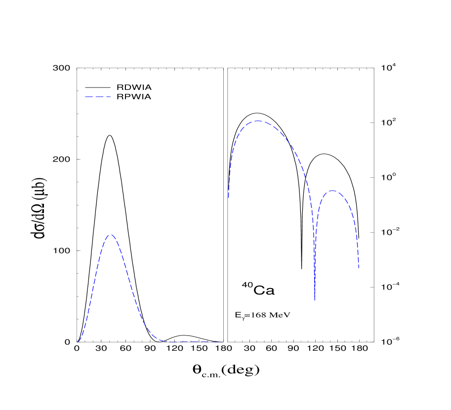
Figure 1: Differential cross section for the coherent pion photoproduction reaction from ${}^{40}\rm{Ca}$ at $E_{\gamma}=168$ MeV using the vector representation for the elementary amplitude with (solid line) and without (dashed line) the inclusion of distortions. Results on the left(right) panel are plotted using a linear(logarithmic) scale.

linear scale) shows the differential cross section for the coherent photoproduction of neutral pions from ${}^{40}\rm{Ca}$ at a laboratory energy of $E_{\gamma}\!=\!168$ MeV. The solid line displays our results using a relativistic distorted-wave impulse approximation (RDWIA) formalism, while the dashed line displays the corresponding plane-wave result (RPWIA). The calculations have been done using a vector representation for the elementary $\gamma N\rightarrow\pi^{0}N$ amplitude. Note that this is only one of the many possible representations of the elementary amplitude that are equivalent on-shell. A detailed discussion of these off-shell ambiguities is deferred to Section 7. At this specific photon energy—one not very far from threshold—the distortions have more than doubled the value of the differential cross section at its maximum. Yet, the shape of the angular distribution seems to be preserved. However, upon closer examination (the right panel of the graph shows the same calculations on a logarithmic scale) we observe that the distortions have caused a substantial back-angle enhancement due to a different sampling of the nuclear density, relative to the plane-wave calculation. This has resulted in a small—but not negligible—shift of about $10^{\circ}$ in the position of the minimum. The back-angle enhancement, with its corresponding shift in the position of the minimum, has been seen in our calculations also at different incident photon energies.

The effect of distortions on the total photoproduction cross section from ${}^{40}\rm{Ca}$ as a function of the photon energy is displayed in Figure 2. The behavior of the distorted cross section is

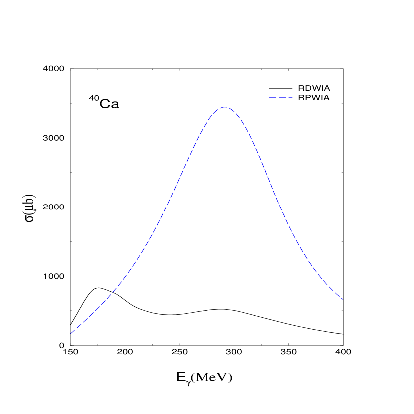
Figure 2: Total cross section for the coherent pion photoproduction reaction from ${}^{40}\rm{Ca}$ as a function of the photon energy in the laboratory frame with (solid line) and without (dashed line) including pionic distortions. A vector representation for the elementary part of the amplitude is used.

explained in terms of a competition between the attractive real (dispersive) part and the absorptive imaginary part of the optical potential. Although the optical potential encompasses very complicated processes, the essence of the physics can be understood in terms of $\Delta$-resonance dominance. Ironically, the behavior of the dispersive and the absorptive parts are caused primarily by the same mechanism: $\Delta$-resonance formation in the nucleus. The mechanism behind the attractive real part is the scattering of the pion from a single nucleon—which is dramatically increased in the $\Delta$-resonance region. In contrast, the absorptive imaginary part is the result of several mechanisms, such as nucleon knock-out, excitation of nuclear states, and two-nucleon processes. At very low energies some of the absorptive channels are not open yet, resulting in a small imaginary part of the potential. This in turn provides a chance for the attractive real part to enhance the coherent cross section. As the energy increases, specifically in the $\Delta$-resonance region, a larger number of absorptive channels become available leading to a large dampening of the cross section. Although the attractive part also increases around the $\Delta$-resonance region, this increase is more than compensated by the absorptive component, which greatly reduces the probability for the pion to interact elastically with the nucleus.

Since understanding pionic distortions constitutes our first step towards a comprehensive study of the coherent process, it is instructive to examine the sensitivity of our results to various theoretical models. To this end, we have calculated the coherent cross section using different optical potentials, all of which fit $\pi$-nucleus scattering data as well as the properties of pionic atoms. We have started by calculating the coherent cross section using the optical potential developed by Carr and collaborators [18]. It should be noted that although our optical potential originates from the work of Carr and collaborators, there are still significant differences between the two sets of optical potentials. These differences arise from the manner in which some parameters are determined and from effects that were not — at least explicitly — included in their model.

In addition to the above potentials, we have calculated the coherent cross section using a simple 4-parameter Kisslinger potential of the form [18]:

$$2\omega U\!=\!-4\pi\left[b_{\rm eff}\rho(r)-c_{\rm eff}\mbox{\boldmath${\nabla}$ \unboldmath}\cdot\rho(r)\mbox{\boldmath${\nabla}$ \unboldmath}+c_{\rm eff}\frac{\omega}{2M_{N}}{\nabla}^{2}\rho(r)\right].$$ (1)

Note that we have used two different sets of parameters for this Kisslinger potential, denoted by K1 and K2 [18]. Both sets were constrained by $\pi$-nucleus scattering data and by the properties of pionic atoms. However, while the K1 fit was constrained to obtain $b_{\rm eff}$ and $c_{\rm eff}$ parameters that did not deviate much from their pionic-atom values, the K2 fit allowed them to vary freely, so as to obtain the best possible fit.

Results for the coherent photoproduction cross section from ${}^{40}\rm{Ca}$ at a photon energy of $E_{\gamma}\!=\!186$ MeV (resulting in the emission of a 50 MeV pion) for the various optical-potential models are shown in Figure 3. In the plot,

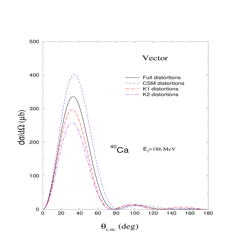
Figure 3: Differential cross section for the coherent pion-photoproduction reaction from ${}^{40}\rm{Ca}$ at $E_{\gamma}\!=\!186$ MeV (resulting in the emission of a 50 MeV pion) using different optical-potential models. All of these models are equivalent insofar as they fit properties of pionic atoms and $\pi$-nucleus scattering data. A vector representation for the elementary part of the amplitude is used.

our results are labeled full-distortions (solid line) while those of Carr, Stricker-Bauer, and McManus as CSM (short dashed line); those obtained with the 4-parameter Kisslinger potential are labeled K1 (long-dashed line) and K2 (dot-dashed line), respectively. It can be seen from the figure that our calculation differs by at most 30% relative to the ones using earlier forms of the optical potential. Note that these results are computed using the vector parameterization of the elementary amplitude. Similar calculations done with the tensor amplitude as can be seen in Figure 4,

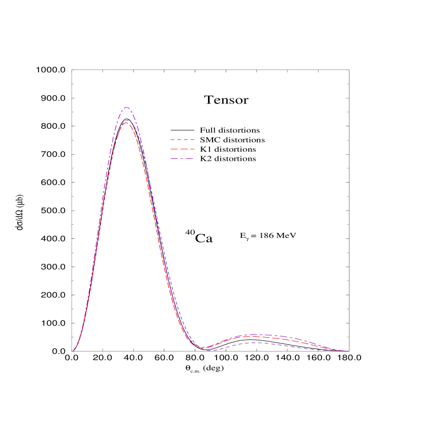
Figure 4: A similar plot to Figure 3 but now with the tensor representation for the elementary part of the amplitude.

display optical-model uncertainties far smaller (of the order of 5%) than the ones reported in Figure 3. In conclusion, although there seems to be a non-negligible uncertainty arising from the optical potential, these uncertainties pale in comparison to the large off-shell ambiguity, to be discussed later on in this chapter.

2 Distortion Effects for the Eta

Distortion effects in the $\eta$ coherent process are also crucial in understanding this process. However, distortions here are not as strong and dramatic as in the case for the pion. Figure 5 displays the

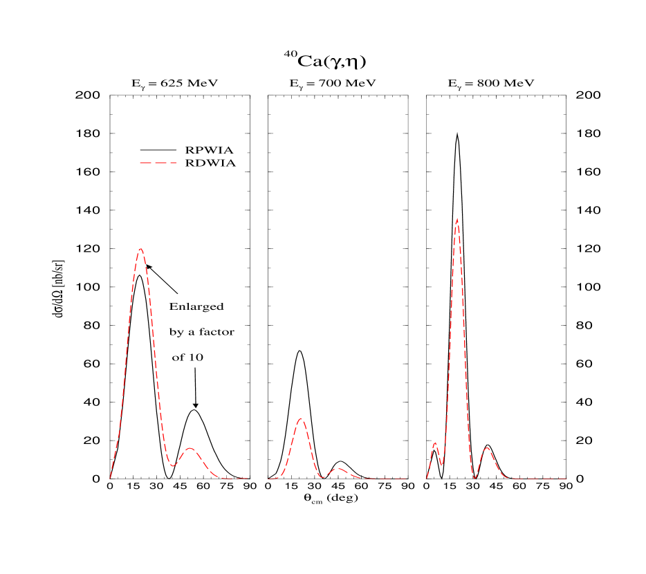
Figure 5: The coherent $\eta$ photoproduction differential cross section from ⁴⁰Ca at photon laboratory energies of $E_{\gamma}=625,700$, and $800$ MeV. The solid lines represent the calculations with no distortions (RPWIA), while the dashed lines represent the same calculations but now with distortions (RDWIA).

coherent $\eta$ photoproduction cross section from ⁴⁰Ca at photon laboratory energies of $E_{\gamma}=625,700,$ and $800$ MeV. The solid lines represent the calculations with no distortions (RPWIA), while the dashed lines represent the same calculations but now with distortions (RDWIA).

The effect of distortions as a function of incident photon energy is manifest in the plot. At low $\eta$ energies (see panel one in Figure 5) the real part of the optical potential is attractive which creates a competition with the absorptive imaginary part of the potential that results in a distorted-wave cross section relatively close to its plane-wave value. At higher energies (see panel two in Figure 5) the real part of the optical potential turns repulsive, and this, in addition to a relatively large imaginary part, results in a large quenching of the distorted cross sections relative to their plane-wave estimations. Finally at $E_{\gamma}\approx 800$ MeV, the effect of distortions is reduced due to a distortion unfavorable strong energy dependence in the $\eta N\rightarrow\eta N$ scattering matrix [10]

2 Relativistic Effects

Having discussed the effects of distortions, I turn now to the effect of relativity. Figure 6 shows the differential cross section

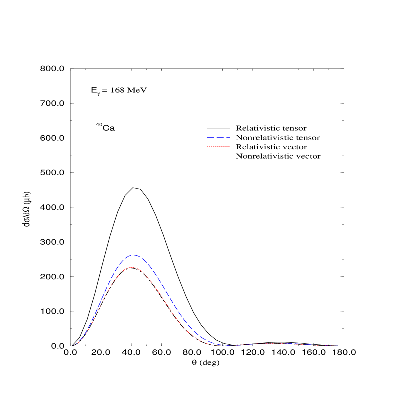
Figure 6: The Differential cross section for the coherent pion-photoproduction reaction from ${}^{40}\rm{Ca}$ at $E_{\gamma}\!=\!168$ MeV calculated using relativistic and nonrelativistic formalisms for both the tensor and vector parameterizations.

for the coherent pion-photoproduction reaction from ${}^{40}\rm{Ca}$ at $E_{\gamma}\!=\!168$ MeV calculated using relativistic and nonrelativistic formalisms for both the tensor and vector parameterizations. The nonrelativistic calculations were obtained by using the free-space relation to relate the lower component to the upper one in the bound-nucleon wavefunction, while keeping the upper component essentially intact apart from a small normalization correction. This method of constructing the nonrelativistic version is our best attempt at reproducing standard nonrelativistic calculations which employ free, on-shell spinors to affect the nonrelativistic reduction of the elementary amplitude.

Figure 6 draws a sharp contrast in the way relativistic effects influence the tensor and vector representations: the tensor parameterization is very sensitive to relativity while the vector one shows outright apathy for it. The tensor cross section experiences a relativistic enhancement by a factor of two. This result is no surprise once we examine the basic definitions of these densities. The tensor one is given by the expression:

$$\rho_{\lower 3.0pt\hbox{$\scriptstyle T$}}(r)=\sum_{a}^{\rm occ}\left({2j_{a}+1\over 4\pi r^{2}}\right)2g_{a}(r)f_{a}(r)\,,$$ (2)

while the vector one is expressed as:

$$\rho_{\lower 3.0pt\hbox{$\scriptstyle V$}}(r)=\sum_{a}^{\rm occ}\left({2j_{a}+1\over 4\pi r^{2}}\right)\Big{[}g_{a}^{2}(r)+f_{a}^{2}(r)\Big{]}\,.$$ (3)

Note that the tensor density is linear in the lower (or small) component of the single-particle wavefunction; this is in contrast to the vector density where the lower component enters as an $(f/g)^{2}$ correction. The mean-field approximation to Walecka model for the nuclear structure is characterized by the existence of large Lorentz scalar and vector potentials that are responsible for a substantial enhancement of the lower components of the single-particle wavefunctions. This enhancement is at the heart of the phenomenological success enjoyed by the Walecka model and is usually referred to as the “$M^{*}$ effect” since the effective mass of the bound nucleon is greatly reduced due to the presence of the large attractive scalar potential. Thus, the large relativistic enhancement of the tensor density represents an inescapable prediction of this model. As we will see throughout this chapter, this is only one facet of the off-shell ambiguity in using one of these representations as opposed to the other one.

3 Effects of Uncertainties in the Nuclear Structure

In order to examine the effects of uncertainties in the nuclear structure, we evaluate the differential cross section using two versions of Walecka model: QHD-I and QHD-II. As has been indicated in Chapter 2, in the QHD-I model the $NN$ interaction is mediated by the $\sigma$ and $\omega$ mesons while in the QHD-II theory we add the photon ($\gamma$) and the $\rho$-meson contributions as well. Figure 7 shows the results of our calculations.

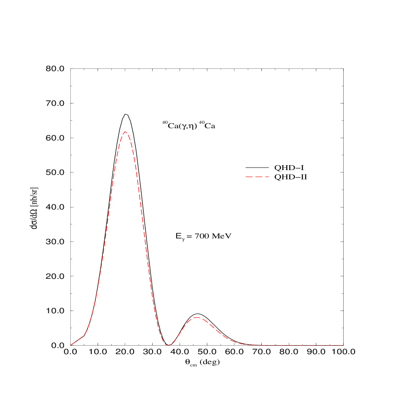
Figure 7: The coherent $\eta$ photoproduction cross section from ⁴⁰Ca at a photon laboratory energy of $E_{\gamma}=700$ MeV. The cross section has been calculated using Walecka QHD-I ($\sigma,\omega$) and QHD-II ($\sigma,\omega,\rho,\gamma$) models.

As can be easily seen, the differential cross section is rather insensitive to which of the two models is used; the results of QHD-I and QHD-II are within ten percent of each other.

4 ${\bf S_{11}}$ Resonance Suppression in the $\eta$ Coherent Process

One of the remarkable results of our study is the suppression of the $S_{11}$ resonance in the $\eta$ coherent process. Figure 8

Figure 8: Breakdown of the elementary contributions to the coherent $\eta$-photoproduction cross section from ⁴⁰Ca at a photon laboratory energy of $E_{\gamma}=700$ MeV. All curves were generated in a relativistic plane-wave-impulse approximation.

displays a breakdown of the elementary contributions to the differential cross section for ⁴⁰Ca using the RPWIA. It is clear that a significant portion of the strength arises from the individual contributions of the $D_{13}$(1520) excitation and the t-channel exchange of vector mesons, while very little strength is contributed by the $S_{11}$(1535) resonance or the Born terms. Also note that the constructive interference between the $D_{13}$(1520) resonance and vector-meson exchange results in a cross section substantially stronger than their incoherent sum.

This result is remarkable because the $S_{11}$ resonance which almost perfectly dominates the cross section for the elementary process (see Figure 3), is strongly suppressed in the coherent process. Thus, the contributions that languish in the darkness of the background in the elementary interaction, spring to life in the coherent process. Consequently, one in principle can use the coherent process to probe and study contributions that cannot be disentangled in elementary processes. For example, it is not clear whether other contributions from resonances that are not included in the elementary process, can be significant in this process. The coherent process can provide us with a tool to determine these background contributions.

5 Effects of Isospin

In most of our calculations of the coherent process, we ignored the isovector component of the reaction amplitude (see Section 6). We have done so because we studied this interaction for nuclei with equal number of protons and neutrons. One valid criticism of our work is that although these nuclei have small isovector densities, there still may be a large isovector component in the reaction amplitude because the $S_{11}$ resonance, which dominates the elementary process but is suppressed in the isoscalar channel, may have a large contribution in the isovector part of the amplitude. For this purpose we have examined the effect of this isovector component as can be seen in Figure 9. The figure decisively shows

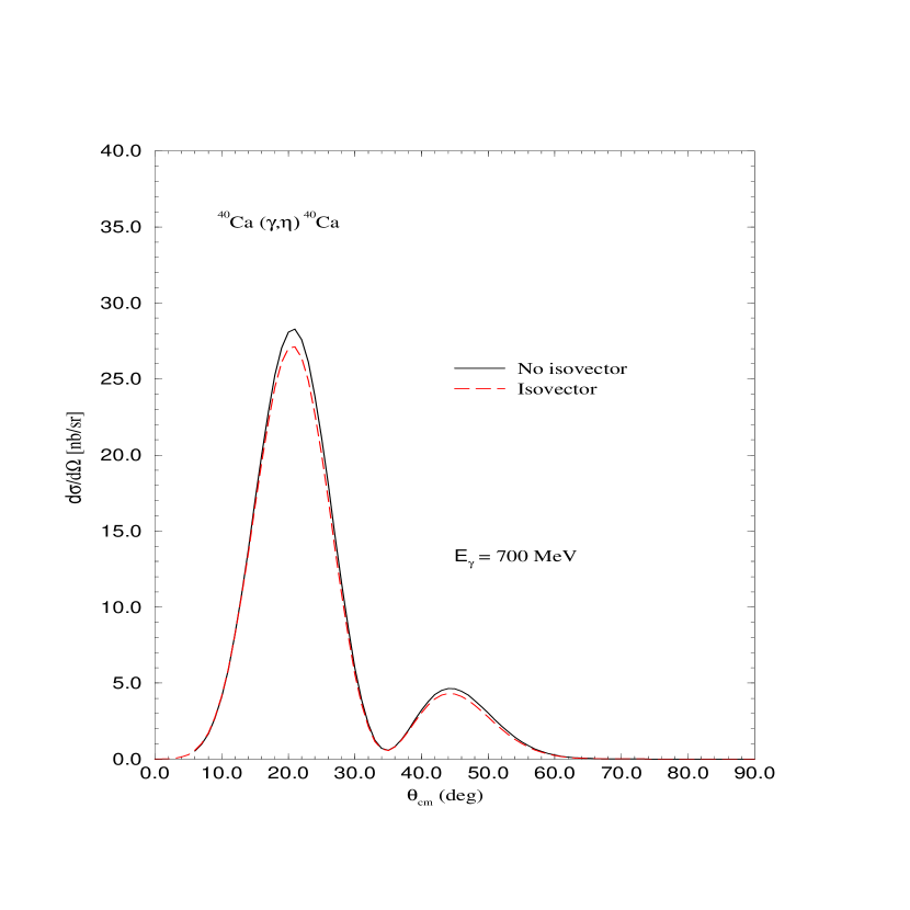
Figure 9: The coherent $\eta$ photoproduction cross section from ⁴⁰Ca at a photon laboratory energy of $E_{\gamma}=700$ MeV. The cross section has been evaluated with no isovector component (solid line) and with isovector component (dashed line).

that this component is insignificant even for ⁴⁰Ca; the nucleus with the largest isovector density among the nuclei that we studied here.

6 Nuclear Dependence of the Coherent Process

The coherent $\eta$ photoproduction differential cross section from ⁴He, ¹²C, and ⁴⁰Ca is shown in Figure 10 at

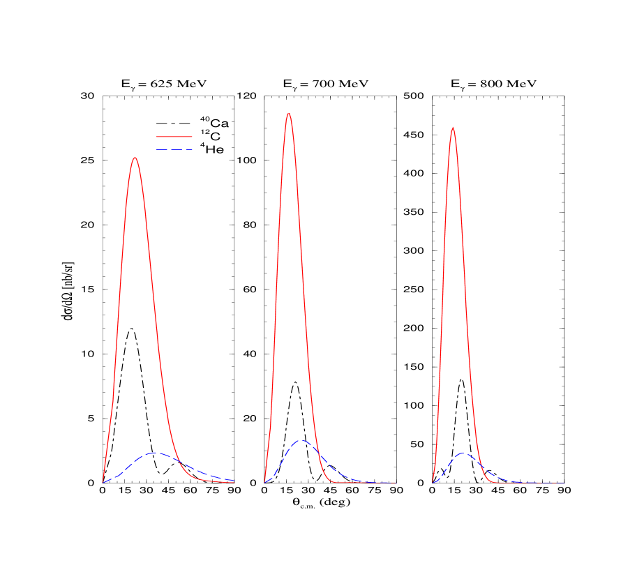
Figure 10: The nuclear dependence of the coherent $\eta$-photoproduction cross section at photon laboratory energies of $E_{\gamma}=625$, $700$ and $800$ MeV in a relativistic distorted-wave-impulse approximation (RDWIA). The calculations have been achieved for three nuclei: ⁴⁰Ca, ¹²C, and ⁴He. ¹²C has the largest cross section of the three nuclei, while ⁴He has the smallest. This result for ¹²C is an example of the open-shell effect (see Section 5). All calculations have been made using the tensor parameterization.

photon laboratory energies of $625$, $700$, and $800$ MeV, respectively. All of these calculations have been achieved using the tensor parameterization. The open-shell effect discussed in Section 5 is manifest in this diagram where the cross section for ¹²C is significantly larger than that for ⁴He and ⁴⁰Ca. Note that ⁴He and ⁴⁰Ca are closed-shell (spin-saturated) nuclei while ¹²C is an open-shell nucleus because its $1p^{1/2}$ orbital is empty while the $1p^{3/2}$ orbital is occupied. It is important to stress here that this open-shell effect is a result of using the tensor representation. It is not present if we would have used the vector one. In this aspect, this is yet another manifestation of the off-shell ambiguity.

The relativistic results shown in this figure differ significantly from those obtained in nonrelativistic calculations. Indeed, Bennhold and Tanabe [10] have predicted that ⁴He would have the largest cross section of the three nuclei, due to its largest charge form factor. This, we believe, might have been an important reason for the selection of ⁴He for the first experimental measurement of the coherent process [51]. However, this finding is at odds with our relativistic results, which instead show ⁴He to have the smallest cross section. There are two main reasons for this difference. First, in relativistic calculations the ratio of upper-to-lower components is determined dynamically in the Walecka model, rather than from its free-space relation. Second, the elementary $\eta N$ interaction used in this work [31, 32] is different from the one used by Bennhold and Tanabe [10], in particular the non-resonant contributions were not considered in the latter. Although both models seems to give an adequate description of the elementary process, important differences emerge in the calculation of the coherent reaction. This is primarily due to the fact that the coherent process from spin-saturated nuclei becomes insensitive to the dominant $S_{11}$(1535) intermediate-resonance contribution, and therefore quite sensitive to the details of other resonant and non-resonant background contributions such as the $D_{13}(1520)$ and vector mesons. Note that our calculations for ⁴He are similar to the nonrelativistic ones reported recently by Fix and Arenhövel’s [13]. However, this agreement seems to be fortuitous, since neither their nuclear-structure model nor their elementary amplitude are similar to ours; their coherent process is dominated by $\omega$-meson exchange, while ours contains, in addition, a significant contribution from the $D_{13}$(1520) resonance.

Finally, there are no experimental data available for the $\eta$ coherent process. However, the theoretical studies of this process have motivated considerable experimental interest which have culminated in an attempt to measure the coherent $\eta$ photoproduction cross section from ⁴He at the Mainz Microtron facility [51]. Possibilities for extensions to higher energies and other nuclei exist, both at the Bonn ELSA facility and at TJNAF [52].

7 Effects of Off-Shell Ambiguity

Now we come to the major obstacle in this work: the off-shell ambiguity. We have already in the previous sections discussed some aspects of this ambiguity as it relates to distortion and relativistic effects and to nuclear dependence. Here, we will discuss other angles of the problem.

We start first by presenting in Figure 11 the

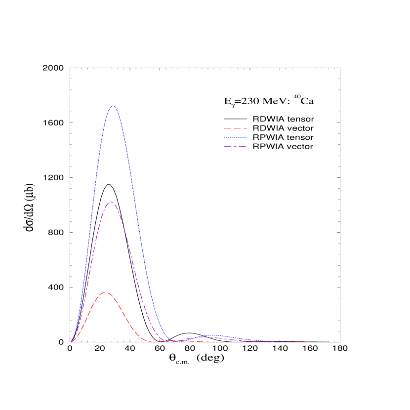
Figure 11: Differential cross section for the coherent pion photoproduction reaction from ${}^{40}\rm{Ca}$ at $E_{\gamma}\!=\!230$ MeV with (RDWIA) and without (RPWIA) pionic distortions. Tensor and vector parameterizations of the elementary amplitude are used.

differential cross section for the coherent photoproduction of neutral pions from ${}^{40}\rm{Ca}$ at a photon energy of $E_{\gamma}\!=\!230$ MeV. Both tensor and vector parameterizations of the elementary amplitude were used, and the cross section was calculated with (RDWIA) and without (RPWIA) pionic distortions. The off-shell ambiguity is immense; factors of two (or more) are observed when comparing the vector and tensor representations. It is important to stress that these calculations were done by using the same nuclear-structure model, the same pionic distortions, and two elementary amplitudes that are identical on-shell. The very large discrepancy between the two theoretical models emerges from the dynamical modification of the Dirac spinors in the nuclear medium, and not from changes to the elementary production amplitude (assessing the impact of medium modifications to the elementary amplitude remains an important open question). Moreover, the large discrepancy between the calculations cannot be attributed to an improper treatment of gauge invariance, as gauge invariance is strictly maintained in all of our calculations (see Equations 7 and 8).

We have compared our theoretical results to preliminary and unpublished data (not shown) provided to us courtesy of B. Krusche [53]. The data follows the same shape as our calculations but the experimental curve seems to straddle the two calculations, although the vector calculation appears closer to the experimental data. This behavior—a closer agreement of the vector calculation to data—has been observed in all of the comparisons that we have done so far.

In Figure 12 we present results for the differential

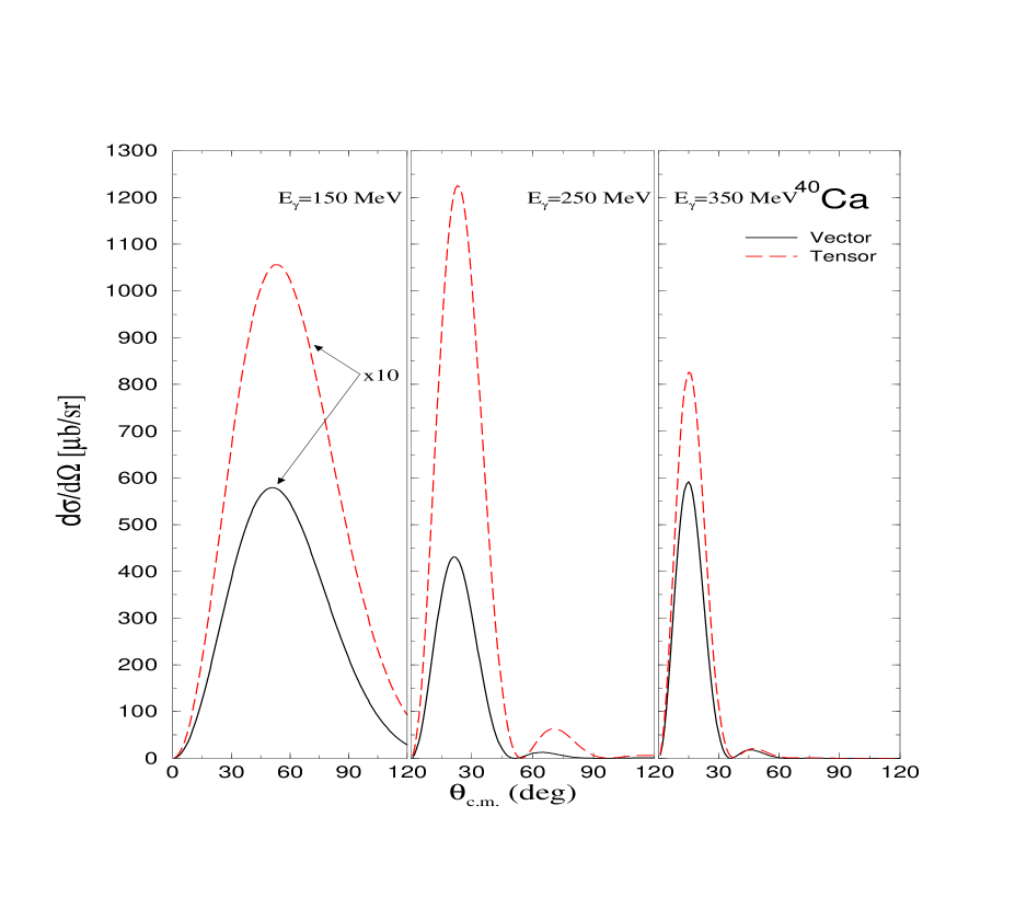
Figure 12: Differential cross section for the coherent pion photoproduction reaction for ${}^{40}\rm{Ca}$ at a variety of photon energies using a RDWIA formalism. Tensor (dashed line) and vector (solid line) parameterizations of the elementary amplitude are used.

cross section from ${}^{40}\rm{Ca}$ at a variety of photon energies, while in Figure 13 we display results for the total cross

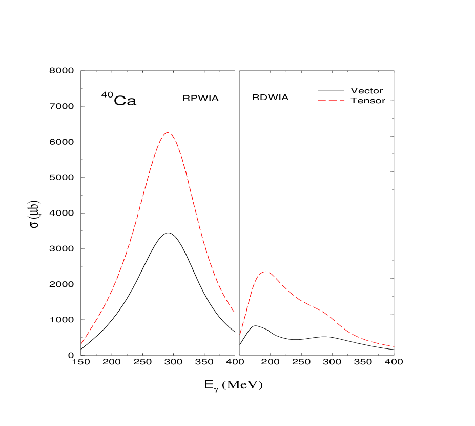
Figure 13: Total cross section for the coherent pion photoproduction reaction from ${}^{40}\rm{Ca}$ as a function of the photon energy with (right panel) and without (left panel) pionic distortions. Tensor (dashed line) and vector (solid line) parameterizations of the elementary amplitude are used.

section. By examining these graphs one can infer that the tensor parameterization always predicts a large enhancement of the cross section—irrespective of the photon incident energy and the scattering angle—relative to the vector predictions. Moreover, the convolution of the tensor and vector densities with the pionic distortions gives rise to similar qualitative, but quite different quantitative, behavior on the energy dependence of the corresponding coherent cross sections.

In Figure 14 we show the differential cross section

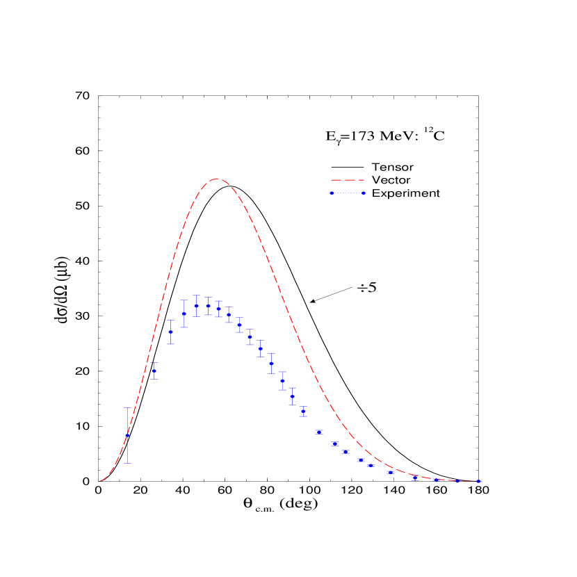
Figure 14: Differential cross section for the coherent pion photoproduction reaction from ${}^{12}\rm{C}$ at $E_{\gamma}\!=\!173$ MeV. Tensor (dashed line) and vector (solid line) parameterizations of the elementary amplitude are used. The experimental data are from Ref. [54].

for the coherent process from ¹²C at a photon energy of $E_{\gamma}\!=\!173$ MeV. The off-shell ambiguity for this case is striking; at this energy the tensor result is five times larger than the vector prediction. The additional enhancement observed here relative to ⁴⁰Ca is easy to understand on the basis of the open-shell effect. Figure 14 also shows a comparison of our results with the experimental data of Ref. [54]. It is clear from the figure that the vector representation is closer to the data; note that the tensor calculation has been divided by a factor of five. Even so, the vector calculation also overestimates the data by a considerable amount.

For further comparison with experimental data we have calculated the coherent cross section from ¹²C at photon energies of $E_{\gamma}\!=\!235$, $250$, and $291$ MeV. In Table 1 we

Table 1: Maxima of the differential cross section (in $\mu$b) for the coherent pion photoproduction reaction from ¹²C at various energies.

$E_{\gamma}$ (MeV)	Tensor	Vector	Experiment
$235$	$694$	$116$	$105$
$250$	$731$	$133$	$190$
$291$	$786$	$186$	$175$

have collated our calculations with experimental data published by Arends and collaborators [55] for $E_{\gamma}\!=\!235$ and $291$ MeV, and with data presented by Booth [56] and Nagl, Devanathan, and Überall [11] for $E_{\gamma\rm{lab}}\!=\!250$ MeV. The experimental data exhibits similar patterns as our calculations (not shown) but the values of the maxima of the cross section are different. The tensor calculations continue to predict large enhancement factors (of five and more) relative to the vector calculations. More importantly, these enhancement factors are in contradiction with experiment. The experimental data appears to indicate that the maximum in the differential cross section from ${}^{12}\rm{C}$ is largest at about $250$ MeV, while our calculations predict a maximum around $295$ MeV. It is likely that this energy “shift” might be the result of the formation and propagation of the $\Delta$-resonance in the nuclear medium. Clearly, in an impulse-approximation framework, medium modifications to the elementary amplitude—arising from changes in resonance properties—can not be accounted for. Yet, a binding-energy correction of about $40$ MeV due to the $\Delta$-nucleus interaction has been suggested before [57]. Indeed, such a shift would also explain the discrepancy in the position of our theoretical cross sections in ⁴⁰Ca, relative to the (unpublished) data by Krusche and collaborators [53]. Moreover, such a shift—albeit of only 15 MeV—was invoked by Peters, Lenske, and Mosel [15] in their recent calculation of the coherent pion-photoproduction cross section. Yet, a detailed study of modifications to hadronic properties in the nuclear medium must go beyond the impulse approximation; a topic outside the scope of the present work. However, a brief qualitative discussion of possible violations to the impulse approximation is given in the next section.

We conclude this section by presenting in Figures 15 and

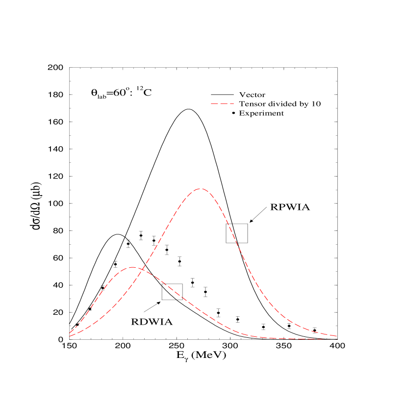
Figure 15: Differential cross section for the coherent pion photoproduction reaction from ${}^{12}\rm{C}$ as a function of photon energy at a fixed laboratory angle of $\theta_{\rm lab}=60^{\circ}$, with and without pionic distortions. Tensor (dashed lines) and vector (solid lines) parameterizations of the elementary amplitude are used. The experimental data are from Ref. [58].

16, a comparison between our plane- and distorted-wave

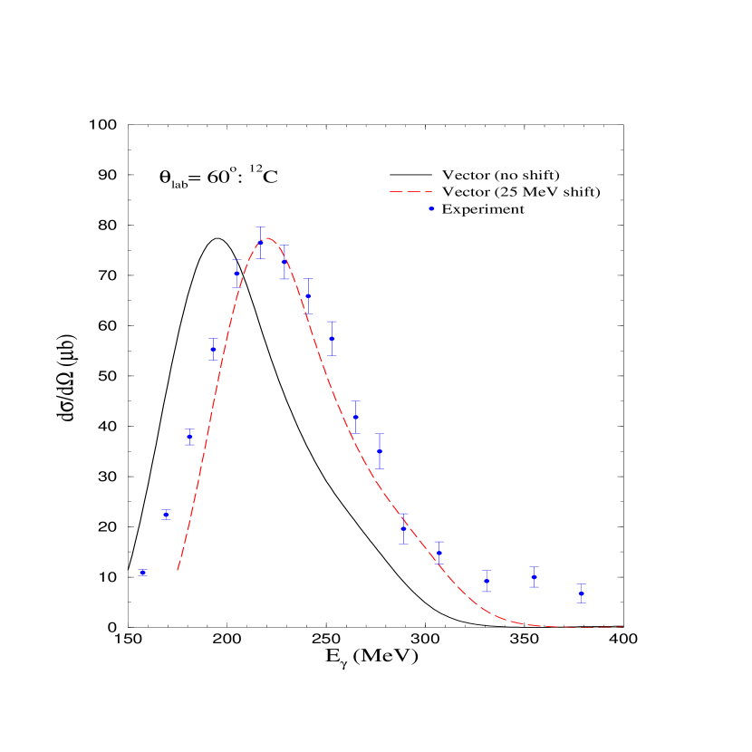
Figure 16: Differential cross section for the coherent pion photoproduction reaction from ${}^{12}\rm{C}$ as a function of photon energy at a fixed laboratory angle of $\theta_{\rm lab}=60^{\circ}$, with pionic distortions and using only a vector parameterization of the elementary amplitude. The same calculation—including a shift of 25 MeV is also included (dashed line). The experimental data are from Ref. [58].

calculations with experimental data for the coherent cross section from ¹²C as a function of photon energy for a fixed angle of $\theta_{\rm lab}\!=\!60^{\circ}$. The experimental data from MAMI is contained in the doctoral dissertation of M. Schmitz [58].

Perhaps the most interesting feature in these figures is the very good agreement between our RDWIA calculation using the vector representation and the data—if we were to shift our results by +25 MeV. Indeed, this effect is most clearly appreciated in Figure 16 where the shifted calculation is now represented by the dashed line. In our treatment of the coherent process, the detailed shape of the cross section as a function of energy results from a delicate interplay between several effects arising from: a) the elementary amplitude—which peaks at the position of the delta resonance ($E_{\gamma}\simeq 340$ MeV from a free nucleon and slightly lower here because of the optimal prescription [2]), b) the nuclear form factor—which peaks at low-momentum transfer, and c) the pionic distortions—which strongly quench the cross sections at high energy, as more open channels become available. We believe that the pionic distortions (see Section 1) as well as the nuclear form factor have been modeled accurately in the present work. The elementary amplitude, although obtained from a recent phase-shift analysis by the VPI group [35], remains one of the biggest uncertainties, as no microscopic model has been used to estimate possible medium modifications to the on-shell amplitude. Evidently, an important modification might arise from the production, propagation, and decay of the $\Delta$-resonance in the nuclear medium. Indeed, a very general result from hadronic physics, obtained from analyses of quasielastic $(p,n)$ and $({}^{3}He,t)$ experiments [57], is that the position of the $\Delta$-peak in nuclear targets is lower relative to the one observed from a free proton target.

However, it is also well known that such a shift is not observed when the $\Delta$-resonance is excited electromagnetically [57]. This apparent discrepancy has been attributed to the different dynamic responses that are being probed by the two processes. In the case of the hadronic process, it is the (pion-like) spin-longitudinal response that is being probed, which is known to get “softened” (shifted to lower excitation energies) in the nuclear medium. Instead, quasielastic electron scattering probes the spin-transverse response—which shows no significant energy shift. Unfortunately, in our present local-impulse-approximation treatment it becomes impossible to assess the effects associated with medium modifications to the $\Delta$-resonance. A detailed study of possible violations to the impulse approximation and to the local assumption remains an important open problem for the future. A qualitative discussion is presented in the next section.

8 Violations to the Impulse Approximation

In this section, we address an additional ambiguity in the formalism, namely, the use of the impulse approximation. The basic assumption behind the impulse approximation is that the interaction in the medium is unchanged relative to its free-space value. The immense simplification that is achieved with this assumption is that the elementary interaction now becomes model independent, as it can be obtained directly from a phase-shift analysis of the experimental data (see, for example, Ref. [35]). The sole remaining question to be answered is the value of $s$ at which the elementary amplitude should be evaluated, as now the target nucleon is not free but rather bound to the nucleus (see Figure 1). This question is resolved by using the “optimal” prescription of Gurvitz, Dedonder, and Amado [42], which suggests that the elementary amplitude should be evaluated in the Breit frame. Then, this optimal form of the impulse approximation leads to a factorizable and local scattering amplitude—with the nuclear-structure information contained in a well-determined form factor. Moreover, as the final-state interaction between the outgoing meson and the nucleus is well constrained from other data, a parameter-free calculation of the coherent photoproduction process ensues.

This form of the impulse approximation has been used with great success in hadronic processes, such as in $(p,p^{\prime})$ and $(p,n)$ reactions, and in electromagnetic processes, such as in electron scattering. Perhaps the main reason behind this success is that the elementary nucleon-nucleon or electron-nucleon interaction is mediated exclusively by $t$-channel exchanges—such as arising from $\gamma$-, $\pi$-, or $\sigma$-exchange. This implies that the local approximation (i.e., the assumption that the nuclear-structure information appears exclusively in the form of a local nuclear form factor) is well justified. For the coherent process this would also be the case if the elementary amplitude would be dominated by the exchange of mesons, as in the last Feynman diagram in Figure 17. However, it is well known—at least for the

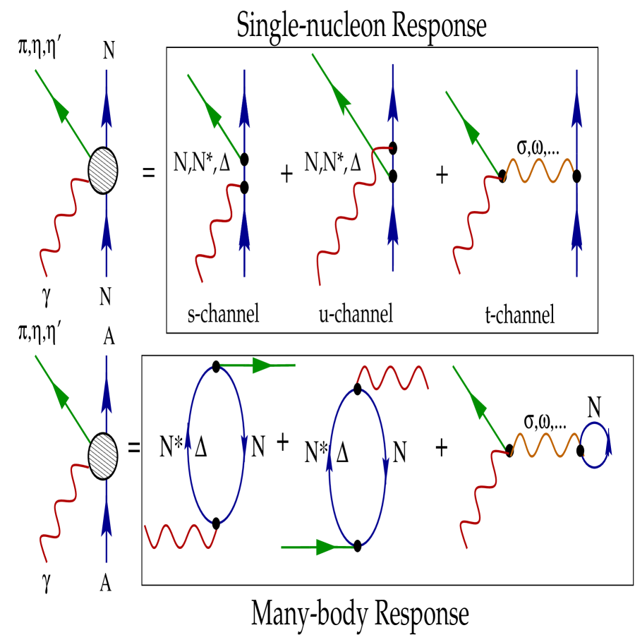
Figure 17: Characteristic s-, u-, and t-channel Feynman diagrams for the photoproduction of pseudoscalar mesons from a single nucleon (upper panel) and—coherently—from the nucleus (lower panel).

kinematical region of current interest—that the elementary photoproduction process is dominated by resonance ($N^{\star}$ or $\Delta$) formation, as in the $s$-channel Feynman diagram of Figure 17. This suggests that the coherent reaction probes, in addition to the nuclear density, the polarization structure of the nucleus (depicted by the “bubbles” in Figure 17). As the polarization structure of the nucleus is sensitive to the ground- as well as to the excited-state properties of the nucleus, its proper inclusion could lead to important corrections to the local impulse-approximation treatment. Indeed, Peters, Lenske, and Mosel have lifted the local assumption and have reported—in contrast to all earlier local studies—that the $S_{11}(1535)$ resonance does contribute to the coherent photoproduction of $\eta$-meson for open-shell (non-spin-saturated) nuclei like ${}^{12}\rm{C}$ [15]. They also reported a significant smearing of the cross section in the case of the $\pi$ coherent process [14]. Clearly, understanding these additional contributions to the coherent process is an important area for future work.

Chapter 6 Conclusions for the Coherent Process

We have studied the coherent photoproduction of pseudoscalar mesons in a relativistic-impulse-approximation approach. We have placed special emphasis on the ambiguities underlying most of the current theoretical approaches. Although our conclusions are of a general nature, we have focused our discussions on the photoproduction of neutral pions due to the “abundance” of data relative to the other pseudoscalar channels.

We have employed a relativistic formalism for the elementary amplitude as well as for the nuclear structure. We believe that, as current relativistic models of nuclear structure rival some of the most sophisticated nonrelativistic ones, there is no longer a need to resort to a nonrelativistic reduction of the elementary amplitude. Rather, the full relativistic structure of the coherent amplitude should be maintained [2, 3, 4].

We have also extended our treatment of the pion-nucleus interaction to the $\Delta$-resonance region. As most of the details about the optical potential will be reported shortly [5], we summarize briefly some of our most important findings. As expected, pionic distortions are of paramount importance. Indeed, we have found a factor-of-two enhancement (at low energies) and up to a factor-of-five reduction (at high energies) in the coherent cross section relative to the plane-wave values. Yet, ambiguities arising from the various choices of optical-model parameters are relatively small; of at most 30%.

We have found important discrepancies vis-a-vis nonrelativistic results [8, 9, 10, 11, 12, 13]. Part of these discrepancies stem from the fact that we have used a fully relativistic approach—with no resort to a nonrelativistic reduction. Moreover, the elementary amplitudes used in our model are different from those used in other theoretical calculations. We found also that the cross section is sensitive to two nuclear-structure quantities: i) the ground-state vector density and ii) the ground-state tensor density. The tensor density is as fundamental as the vector density used in the nonrelativistic treatments, although it is not as well constrained by experiment.

By far the largest uncertainty in our results emerges from the ambiguity in extending the many—actually infinite—equivalent representations of the elementary amplitude off the mass shell. While all these choices are guaranteed to give identical results for on-shell observables, they yield vastly different predictions off-shell. Yet, it is worth mentioning that the off-shell ambiguity emerges mainly from our insistence in using the impulse approximation. With an effective microscopic model—calibrated to reproduce two- and many-body scattering amplitudes—the off-shell ambiguity can, to a large extent, be removed. This task, however, remains a formidable one—forcing us, as well as most existing theoretical approaches, to rely on the impulse approximation.

In this work we have investigated two on-shell-equivalent representations of the elementary amplitude: a tensor and a vector. The tensor representation employs the “standard” form of the elementary amplitude [10, 16] and generates a coherent photoproduction amplitude that is proportional to the isoscalar tensor density. However, this form of the elementary amplitude, although standard, is not unique. Indeed, through a simple manipulation of operators between on-shell Dirac spinors, the tensor representation can be transformed into the vector one, so-labeled because the resulting coherent amplitude becomes proportional now to the isoscalar vector density. The tensor and vector densities were computed in a self-consistent, mean-field approximation to the Walecka model [17]. The Walecka model is characterized by the existence of large Lorentz scalar and vector potentials that are responsible for a large enhancement of the lower components of the single-particle wave functions. This so-called “$M^{\star}$-enhancement” generates a large increase in the tensor density, as compared to a scheme in which the lower component is computed from the free-space relation. No such enhancement is observed in the vector representation, as the vector density is insensitive to the $M^{\star}$-effect. As a result, the tensor calculation predicts coherent photoproduction cross sections that are up to an order of magnitude larger than the vector results. These large enhancement factors are not consistent with existent experimental data. Still, it is important to note that the vastly different predictions of the two models have been obtained using the same pionic distortions, the same nuclear-structure model, and two sets of elementary amplitudes that are identical on-shell.

Finally, we have addressed—in a qualitative fashion—violations to the impulse approximation. In the impulse approximation one assumes that the elementary amplitude may be used without modification in the nuclear medium. Moreover, by adopting the optimal prescription of Ref. [42], one arrives at a form for the coherent amplitude that is local and factorizable. Indeed, such an optimal form has been used extensively—and with considerable success—in electron and nucleon elastic scattering from nuclei. We suggested here that the reason behind such a success is the $t$-channel–dominance of these processes. In contrast, the coherent-photoproduction process is dominated by resonance formation in the $s$-channel. In the nuclear medium a variety of processes may affect the formation, propagation, and decay of these resonances. Thus, resonant-dominated processes may not be amenable to treatment via the impulse-approximation. Further, in $s$-channel–dominated processes, it is not the local nuclear density that is probed, but rather, it is the (non-local) polarization structure of the nucleus. This can lead to important deviations from the naive local picture. Indeed, by relaxing the local assumption, Peters and collaborators have reported a non-negligible contribution from the $S_{11}(1535)$ resonance to the coherent $\eta$ process for open-shell nuclei [15], and a significant smearing of the cross section in the case of the $\pi$ coherent process [14].

In summary, we have studied a variety of sources that challenge earlier studies of the coherent photoproduction of pseudoscalar mesons. Without a clear understanding of these issues, erroneous conclusions are likely to be extracted from the wealth of experimental data that will soon become available. Undoubtedly, there is still a lot of work to be done both experimentally and theoretically. Indeed, many challenging and interesting lessons have yet to be learned before a deep understanding of the coherent-photoproduction process will emerge. We hope that with the advent of new powerful and sophisticated facilities, such as TJNAF and MAMI, the validity of the different theoretical models can be tested.

Chapter 7 Theory of the Quasifree Meson Photoproduction from Nuclei

This chapter and the next two will be devoted to a study of the theory of the quasifree meson photoproduction from nuclei. This process consists of a photon ($\gamma$-ray) incident on a nucleus. The photon interacts with the nucleus and as a result a pseudoscalar meson is produced (like $K^{+}$, $\pi$, or $\eta$) through knocking out one of the nucleons. In the case of the $K^{+}$ quasifree process that we will study here, a proton is knocked out into one of its excited states: the $\Lambda$ hyperon. Thus, we start the interaction with a photon and some nucleus, and end up with a meson, a free nucleon or a hyperon, and a new recoil nucleus. This process is labeled as “quasifree” because the interaction occurs in a similar kinematic setting to the free process of $N(\gamma,PS\,\,meson)N(Y)$. Specifically, the energy transfer $\omega$ is related to the momentum transfer ${\mathbf{q}}$ (as in the free process) according to the equation

$$\omega\!=\!\sqrt{{\mathbf{q}}^{2}+M_{\Lambda}^{2}}-M_{N}\;.$$ (1)

This equation defines what is usually called the “quasifree condition”.

Furthermore, this process is perceived to take place from only one of the nucleons in the nucleus. In this aspect, it is identical to the elementary process except in the fact that the target nucleon is bound as opposed to being free. Due to this similarity, it is no surprise that this interaction is our best attempt to obtain insights into the nature of the elementary process in slightly different circumstances.

1 Basic Ingredients

As in the case for the coherent process, we employ the relativistic impulse approximation. However, we do not incorporate any distortions to the emitted meson or to the outgoing nucleon (hyperon). In other words, we study this interaction in the framework of the relativistic plane-wave impulse approximation (RPWIA). Figure 1 provides a schematic diagram for the kaon quasifree process within this approximation.

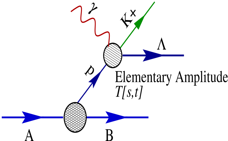
Figure 1: A representation of the quasifree photoproduction of a $\Lambda$-hyperon in a plane-wave impulse-approximation approach.

The rationale for not including distortions is due to our interest in the polarization observables which are insensitive to distortion effects. Indeed, earlier nonrelativistic calculations [23, 24, 25] have demonstrated that two important polarization observables — the recoil polarization of the ejected nucleon (hyperon) and the photon asymmetry — are largely insensitive to distortion effects. Moreover, they seem to be also independent of the mass of the target nucleus. Polarization observables carry the richest information about the fundamental physics in this process, and they are far more effective discriminators of subtle dynamics than the unpolarized cross section. Finally, and in practical terms, ignoring distortions results in an enormous simplification in the formalism of this process.

We maintain the full relativistic structure whether in the elementary photoproduction or in the nuclear structure. This approach forms a significant departure from the traditional nonrelativistic studies [23, 24, 25]. Indeed, RPWIA calculations have been successful in identifying physics not present at the nonrelativistic level. For example, relativistic effects have been shown to contaminate any attempt to infer color transparency from a measurement of the asymmetry in the $(e,e^{\prime}p)$ reaction [26]. Further, the well-known factorization limit of nonrelativistic plane-wave calculations has been shown to break down due to the presence of negative-energy components in the bound-nucleon wavefunction[27].

2 Observables

The differential cross section is derived using well-established procedures [41]. Note however that we have here three particles in the final state as opposed to two in the coherent process. As a result, the differential cross section (in the lab system) is expressed as:

$${\left[d^{5}\sigma(s^{\prime},\epsilon)\right]}_{\rm lab}=\frac{1}{2E_{\gamma}}\;(2\pi)^{4}\;\delta^{4}(k+p_{A}-k^{\prime}-p^{\prime}-p_{B})\;{\big{|}{\cal M}\big{|}}^{2}\;\frac{d^{3}{\bf k}^{\prime}}{(2\pi)^{3}2E_{{\bf k}^{\prime}}}\frac{M_{N(\Lambda)}d^{3}{\bf p}^{\prime}}{(2\pi)^{3}2E_{{\bf p}^{\prime}}}\frac{d^{3}{\bf p}_{B}}{(2\pi)^{3}}\;,$$ (2)

where $k$ is the four-momentum of the incident photon, while $k^{\prime}$ and $p^{\prime}$ are the momenta of the produced meson and nucleon (hyperon), respectively. Here, $p_{A}$($p_{B}$) represents the momentum of the target(residual) nucleus. Finally, $s^{\prime}$ is the spin of the emitted nucleon (hyperon), $\epsilon$ is the polarization of the incident photon, $M_{N(Y)}$ is the nucleon (hyperon) mass, and ${\cal M}$ is the transition matrix element.

By integrating over the delta function, we obtain the following form for the differential cross section:

$$\left(\frac{d^{5}\sigma(s^{\prime},\epsilon)}{d{k}^{\prime}d\Omega_{{\bf k}^{\prime}}d\Omega_{{\bf p}^{\prime}}}\right)_{\rm lab}=\frac{2\pi}{2E_{\gamma}}\mbox{ }\frac{|{\bf k}^{\prime}|^{2}}{(2\pi)^{3}\,2E_{{\bf k}^{\prime}}}\mbox{ }\frac{M_{N(Y)}|{\bf p}^{\prime}|}{(2\pi)^{3}}\mbox{ }{\big{|}{\cal M}\big{|}}^{2}\;.$$ (3)

The unpolarized differential expression can be obtained by summing over the two possible components of the spin of the nucleon (hyperon) and averaging over the transverse photon polarization. That is,

$$\left(\frac{d^{5}\sigma}{d{k}^{\prime}d\Omega_{{\bf k}^{\prime}}d\Omega_{{\bf p}^{\prime}}}\right)_{\rm lab}=\frac{1}{2}\sum_{s^{\prime},\epsilon}\left(\frac{d^{5}\sigma(s^{\prime},\epsilon)}{d{k}^{\prime}d\Omega_{{\bf k}^{\prime}}d\Omega_{{\bf p}^{\prime}}}\right)_{\rm lab}\;.$$ (4)

Yet, our prime interest in this work is the calculation of polarization observables: the recoil $N(Y)$-polarization (${\cal P}$) and the photon asymmetry ($\Sigma$). The former is defined as [11, 28, 29]

$${\cal P}=\sum_{\epsilon}\left(\frac{{d^{5}\sigma}(\uparrow)-{d^{5}\sigma}(\downarrow)}{{d^{5}\sigma}(\uparrow)+{d^{5}\sigma}(\downarrow)}\right)_{\rm lab}\;,$$ (5)

while the latter by [24, 25, 29]

$${\Sigma}=\sum_{s^{\prime}}\left(\frac{{d^{5}\sigma}(\perp)-{d^{5}\sigma}(\parallel)}{{d^{5}\sigma}(\perp)+{d^{5}\sigma}(\parallel)}\right)_{\rm lab}\;.$$ (6)

In these expressions $\uparrow$ and $\downarrow$ represent the projection of the spin of the $N(Y)$-hyperon with respect to the normal to the scattering plane (${\bf k}\times{\bf k}^{\prime}$), while $\perp$($\parallel$) represents the out-of-plane(in-plane) polarization of the photon.

It can be shown that the differential element $d^{5}\sigma$ can be written as $Z^{\mu}Z_{\nu}\epsilon_{\mu}\epsilon^{\nu}$, where $Z_{\mu}$ is some coefficient . This fact allows us to derive a more useful expression for $\Sigma$ as

$${\Sigma}=\left(\frac{2{d^{5}\sigma}(\perp)/d{k}^{\prime}d\Omega_{{\bf k}^{\prime}}d\Omega_{{\bf p}^{\prime}}}{{d^{5}\sigma}/d{k}^{\prime}d\Omega_{{\bf k}^{\prime}}d\Omega_{{\bf p}^{\prime}}}\right)_{\rm lab}-1\;.$$ (7)

Therefore, this observable is related to the ratio of twice the cross section for out-of-plane polarization divided by the unpolarized cross section.

3 Elementary ($\gamma p\rightarrow K^{+}\Lambda$) Amplitude

As I have indicated above, we will study in this work only the kaon quasifree process: $A(\gamma,K^{+}\Lambda)B$. For the elementary photoproduction amplitude we have used the standard model-independent parameterization (see Chapter 1) as following:

$$T(\gamma p\rightarrow K^{+}\Lambda)=F^{\alpha\beta}_{T}\sigma_{\alpha\beta}+iF_{P}\gamma_{5}+F^{\alpha}_{A}\gamma_{\alpha}\gamma_{5}\;,$$ (8)

where we have tensor, pseudoscalar, and axialvector components. Note that in the presently-adopted parameterization, no scalar nor vector invariants appear.

For our calculations we use various different models for the elementary process. These include the hadronic model developed by Williams, Ji, and Cotanch[28]. These authors impose crossing symmetry in their model to develop phenomenologically consistent strong-coupling parameterizations which simultaneously describe the kaon-photoproduction and radiative-capture reactions. Although these are theoretically sound, other choices for the elementary amplitude — more sophisticated and up to date — have also been adopted. In particular, we use the “Saclay-Lyon-Collaboration” model developed by David, Fayard, Lamot, and Saghai[29]. This model is based on an isobaric treatment using low-order Feynman amplitudes that include nucleonic (spin $\leq$ 5/2), hyperonic (spin 1/2), and kaonic resonances. Recently, this model has been extended by T. Mizutani, C. Fayard, G.H. Lamot, and B. Saghai to incorporate off-shell effects implied in any treatment of fermions with spin $\geq 3/2$ [36]. In their approach two different models were obtained. The first one (labeled Model B) is based on a simplified version of the Saclay-Lyon-Collaboration model — the $N(1440)$ and $N(1675)$ resonances have been removed — but it includes an off-shell treatment for the only retained spin-3/2 resonance [$N(1720)$] in the reaction mechanism. The second one (Model C) is identical to Model B, except for the addition of an extra spin-3/2 hyperonic resonance [$\Lambda(1890)$] and its off-shell behavior. In referring to the various models we have adopted the following conventions: the model of the Saclay-Lyon Collaboration is labeled by SL, while Model B and Model C are labeled as SLB and SLC, respectively. Finally, WJC labels the model by Williams, Ji, and Cotanch. Note that the SL model will be used in all of our calculations, unless stated otherwise.

4 Scattering Matrix Element

In a similar fashion to the coherent process, the most general expression for the scattering matrix element in the framework of the RPWIA can be written as a multiple integral in the following form:

$$\int d^{4}x_{1}\ldots d^{4}x_{N}\;\overline{{\psi}}\;A^{\mu}J_{\mu}(x_{1},\ldots,x_{N})\;{\cal U}_{\alpha}\;\phi\;,$$ (9)

where ${\cal U}_{\alpha}$ is a single-particle Dirac spinor for the bound nucleon, $\psi$ is the Dirac spinor for the outgoing nucleon (hyperon), $A^{\mu}$ is the photon wavefunction, and $\phi$ is the pseudoscalar meson wavefunction. The number $N$ of the independent variables to be integrated over depends on the nature of the effective field theory employed. It can be shown that this expression can be reduced to the following form:

$$\big{|}{\cal M}\big{|}^{2}=\delta(p^{0}+k^{0}-p^{\prime 0}-k^{\prime 0})\sum_{m}\Big{|}\overline{\cal U}({\bf p}^{\prime},s^{\prime})\mbox{ }T(s,t)\mbox{ }{\cal U}_{\alpha,m}({\bf p})\Big{|}^{2}\;.$$ (10)

Here ${\cal U}({\bf p}^{\prime},s^{\prime})$ is the free Dirac spinor for the emitted $\Lambda$-hyperon and ${\cal U}_{\alpha,m}({\bf p})$ is the Fourier transform of the relativistic spinor for the bound nucleon [$\alpha$ denotes the collection of all quantum numbers necessary (besides $m$) to specify the single-particle orbital]. Note that since we assume that the impulse approximation is valid, we employ the on-shell photoproduction operator $T(s,t)$ as given by Equation 8.

The nucleon bound-state wavefunction can be expressed in a two component representation as following (see Chapter 2),

$${\cal U}_{E\kappa m}({\bf x})=\frac{1}{x}\left[\begin{array}[]{c}g_{E\kappa}(x){\cal Y}_{+\kappa\mbox{}m}(\hat{\bf x})\\ if_{E\kappa}(x){\cal Y}_{-\kappa\mbox{}m}(\hat{\bf x})\end{array}\right]\;,$$ (11)

where the spin-angular functions are defined as:

$${\cal Y}_{\kappa\mbox{}m}(\hat{\bf x})\equiv\langle{\hat{\bf x}}|l{\scriptstyle\frac{1}{2}}jm>\;;\quad j=|\kappa|-\frac{1}{2}\;;\quad l=\cases{\kappa\;,&if $\kappa>0\;$;\cr-1-\kappa\;,&if $\kappa<0\;$.\cr}$$ (12)

The Fourier transform of the relativistic bound-state wavefunction can now be evaluated . We obtain,

$${\cal U}_{E\kappa m}({\bf p})\equiv\int d{\bf x}\;e^{-i{\bf p}\cdot{\bf x}}\;{\cal U}_{E\kappa m}({\bf x})={4\pi\over p}(-i)^{l}\left[\begin{array}[]{c}g_{E\kappa}(p)\\ f_{E\kappa}(p)({\bf\sigma}\cdot{\hat{\bf p}})\end{array}\right]{\cal{Y}}_{+\kappa m}(\hat{\bf{p}})\;,$$ (13)

where we have written the Fourier transforms of the radial wavefunctions as

$$g_{E\kappa}(p) = \int_{0}^{\infty}dx\,g_{E\kappa}(x)\hat{\jmath}{\hbox{\lower 3.0pt\hbox{${}_{l}$}}}(px)\;,$$ (14)

$$f_{E\kappa}(p) = ({\rm sgn}\kappa)\int_{0}^{\infty}dx\,f_{E\kappa}(x)\hat{\jmath}{\hbox{\lower 3.0pt\hbox{${}_{l^{\prime}}$}}}(px)\;.$$ (15)

Note that in the above expressions we have introduced the Riccati-Bessel function in terms of the spherical Bessel function [59]: $\hat{\jmath}{\hbox{\lower 3.0pt\hbox{${}_{l}$}}}(z)=zj{\hbox{\lower 3.0pt\hbox{${}_{l}$}}}(z)$, and that $l^{\prime}$ is the orbital angular momentum corresponding to $-\kappa$ (see Equation 12).

Since the scattering matrix element is proportional to the bound-nucleon wavefunction in momentum space, it is instructive to examine the momentum content of the wavefunction.

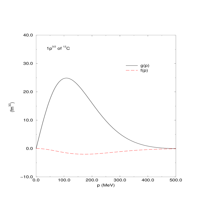
Figure 2: $g_{E\kappa}(p)$ and $f_{E\kappa}(p)$: the radial components of the bound-nucleon wavefunction in momentum space for the $1p^{3/2}$ orbital of ¹²C.

Figure 2 shows $g_{E\kappa}(p)$ and $f_{E\kappa}(p)$ as a function of momentum for the $1p^{3/2}$ orbital of ¹²C. It is evident here that the wavefunction has its maximum around $100$ MeV and that it is appreciable only for $p\leq 300$ MeV.

5 Closed-form Expression for the Photoproduction Amplitude

Having introduced all relevant quantities, we are now in a position to evaluate the (square of the) photoproduction amplitude (Equation 10). Without distortions, the evaluation of the $\Lambda$ propagator is now standard due to an algebraic “trick” that appears to be used for the first time by Casimir [60, 61]:

$$S(p^{\prime})\equiv\sum_{s^{\prime}}{\cal U}({\bf p}^{\prime},s^{\prime})\,\overline{{\cal U}}({\bf p}^{\prime},s^{\prime})=\frac{\hbox to0.0pt{/\hss}p^{\prime}+M_{\Lambda}}{2M_{\Lambda}}\;;\quad\left(p^{\prime\,0}\equiv E_{\Lambda}({\bf p}^{\prime})=\sqrt{{\bf p}^{\prime\,2}+M_{\Lambda}^{2}}\right)\;.$$ (16)

Subsequently others — Feynman being apparently the first one — used this trick to reduce the “complex” computation of covariant matrix elements to a simple and elegant evaluation of traces of Dirac $\gamma$-matrices. These trace-techniques have been used here to compute free polarization observables (note that free polarization observables will serve as the baseline for comparison against bound-nucleon calculations). In principle, one does not expect that these useful trace-techniques will generalize once the nucleon goes off its mass shell. Yet, simple algebraic manipulations — first performed to our knowledge by Gardner and Piekarewicz [26] — show that a trick similar to that of Casimir holds even for bound spinors. Indeed, the validity of their result rests on the following simple identity:

$$\sum_{m}{\cal{Y}}_{+\kappa m}(\hat{\bf{p}}){\cal{Y}}^{*}_{\pm\kappa m}(\hat{\bf{p}})=\pm\frac{2j+1}{8\pi}\cases{1\cr{\bf\sigma}\cdot\hat{\bf p}\cr}\;,$$ (17)

which enables one to introduce the notion of a “bound-state propagator”. That is,

$$S_{\alpha}({\bf p}) \equiv {1\over 2j+1}\sum_{m}{\cal U}_{\alpha,m}({\bf p})\,\overline{\cal U}_{\alpha,m}({\bf p})$$ (20)

$$= \left({2\pi\over p^{2}}\right)\left(\begin{array}[]{cc}g^{2}_{\alpha}(p)&-g_{\alpha}(p)f_{\alpha}(p){\bf\sigma}\cdot{\hat{\bf p}}\\ +g_{\alpha}(p)f_{\alpha}(p){\bf\sigma}\cdot{\hat{\bf p}}&-f^{2}_{\alpha}(p)\end{array}\right)$$

$$= ({\hbox to0.0pt{/\hss}{p}}_{\alpha}+M_{\alpha})\;,\quad\Big{(}\alpha=\{E,\kappa\}\Big{)}\;.$$ (21)

Note that we have defined the above mass-, energy-, and momentum-like quantities as

$$M_{\alpha} = \left({\pi\over p^{2}}\right)\Big{[}g_{\alpha}^{2}(p)-f_{\alpha}^{2}(p)\Big{]}\;,$$ (22)

$$E_{\alpha} = \left({\pi\over p^{2}}\right)\Big{[}g_{\alpha}^{2}(p)+f_{\alpha}^{2}(p)\Big{]}\;,$$ (23)

$${\bf p}_{\alpha} = \left({\pi\over p^{2}}\right)\Big{[}2g_{\alpha}(p)f_{\alpha}(p)\hat{\bf p}\Big{]}\;,$$ (24)

which satisfy the “on-shell relation”

$$p_{\alpha}^{2}=E_{\alpha}^{2}-{\bf p}_{\alpha}^{2}=M_{\alpha}^{2}\;.$$ (25)

The evident similarity in structure between the free and bound propagators (Equations 16 and 21) results in an enormous simplification; we can now employ the powerful trace techniques developed by Feynman to evaluate all polarization observables — irrespective of whether the nucleon is free or bound to a nucleus. It is important to note, however, that this enormous simplification would have been lost if distortion effects would have been incorporated in the propagation of the emitted $\Lambda$-hyperon.

It is informative to examine the behavior and significance of the mass-, energy-, and momentum-like quantities: $M_{\alpha}$, $E_{\alpha}$, and ${\bf p}_{\alpha}$. Figure 3 exhibits these variables as a function of momentum.

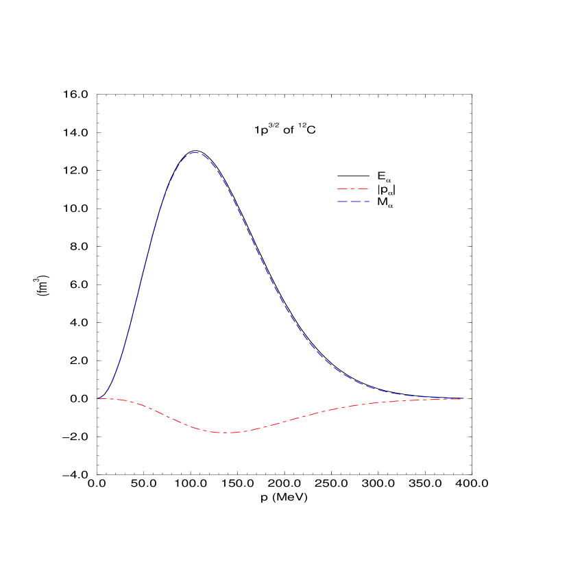
Figure 3: The effective mass-, energy-, and momentum-like quantities: $M_{\alpha}$, $E_{\alpha}$, and $|{\bf p}_{\alpha}|$ as a function of the momentum ($p$).

Note that $|{\bf p}_{\alpha}|\ll E_{\alpha}$ and $M_{\alpha}\simeq E_{\alpha}$. This is a consequence of the fact that $f_{\alpha}(p)$, although enhanced in the nuclear medium, is still much smaller than $g_{\alpha}(p)$. Since the cross section is proportional to the term (${\hbox to0.0pt{/\hss}{p}}_{\alpha}+M_{\alpha}$), and since $|{\bf p}_{\alpha}|\ll E_{\alpha}$ and $M_{\alpha}\simeq E_{\alpha}$, the cross section becomes directly proportional to $E_{\alpha}$. This is a pleasant outcome as $E_{\alpha}$ has a simple interpretation as the bound-nucleon density in momentum space (see Equation 23). Therefore, we deduce that the quasifree process provides us with a direct probe of the momentum distribution in the bound-nucleon wavefunction.

To provide a feeling for the enormous simplification entailed by the above trick, we derive now an example assuming, for mere simplicity, that the photoproduction amplitude contains only the tensor term ($\sigma_{\alpha\beta}$ term in Equation 8). For this case the square of the unpolarized photoproduction matrix element (Equation 10) becomes proportional to:

$$\big{|}{\cal M}\big{|}^{2} \rightarrow |A_{1}|^{2}\,\left(-\frac{1}{2}g_{\mu\nu}\right)\,T{\hbox{\lower 2.0pt\hbox{$r$}}}\Big{[}\gamma^{5}\gamma^{\mu}\hbox to0.0pt{/\hss}k\left(\hbox to0.0pt{/\hss}p_{\alpha}+M_{\alpha}\right)\gamma^{5}\gamma^{\nu}\hbox to0.0pt{/\hss}k\left(\hbox to0.0pt{/\hss}p^{\prime}+M_{\Lambda}\right)\Big{]}$$ (26)

$$= \frac{1}{2}\,|A_{1}|^{2}\left[T{\hbox{\lower 2.0pt\hbox{$r$}}}\Big{(}\gamma^{\mu}\hbox to0.0pt{/\hss}k\hbox to0.0pt{/\hss}p_{\alpha}\gamma_{\mu}\hbox to0.0pt{/\hss}k\hbox to0.0pt{/\hss}p^{\prime}\Big{)}-M_{\alpha}M_{\Lambda}T{\hbox{\lower 2.0pt\hbox{$r$}}}\Big{(}\gamma^{\mu}\hbox to0.0pt{/\hss}k\gamma_{\mu}\hbox to0.0pt{/\hss}k\Big{)}\right]$$

$$= 8\,|A_{1}|^{2}(k\cdot p_{\alpha})(k\cdot p^{\prime})\;.$$

This result is, indeed, simple and illuminating. Although including the full complexity of the elementary amplitude requires the evaluation of thirty-two such terms (not all of them independent) the evaluation of any one of those terms is not much more complicated than the one presented above. Yet, to automate this straightforward but lengthy procedure, we rely on the FeynCalc 1.0[62] package with Mathematica 2.0 to calculate all traces involving $\gamma$-matrices. The output from these symbolic manipulations was then fed into a FORTRAN code to obtain the final numerical values for all different polarization observables. In the appendix, I include full calculations of the traces of $\gamma$-matrices for the generalized case involving two fermions, one of which is polarized while the other one is not.

6 Kinematics in the Quasifree Process

The kinematics for the quasifree production of a $\Lambda$-hyperon through the photoproduction reaction $A(\gamma,K^{+}\Lambda)B$ is constrained by two conditions. First, there is an overall energy-momentum conservation:

$$k+p_{A}=k^{\prime}+p^{\prime}+p_{B}\;.$$ (27)

Moreover, since we are studying the photoproduction process within the framework of the impulse approximation (see Figure 1) there is a second kinematical constraint arising from energy-momentum conservation at the $\gamma N\!\rightarrow\!K^{+}\Lambda$ vertex:

$$k+p=k^{\prime}+p^{\,\prime}\;,$$ (28)

where $p$ is the four-momentum of the bound nucleon, whose space part is known as the missing momentum:

$${\bf p}_{m}\equiv{\bf p}^{\,\prime}-{\bf q}\;;\quad({\bf q}\equiv{\bf k}-{\bf k}^{\prime})\;.$$ (29)

Thus, as in most semi-inclusive processes — such as in the $(e,e^{\prime}p)$ reaction — the quasifree production process becomes sensitive to the nucleon momentum distribution.

The kinematic structure of the quasifree process is much richer than that of the free process. The reason is that the target nucleon is bound and thus has a distribution of momentum states as opposed to only one specific state. This adds more degrees of freedom for the outgoing particles which can now be in states that are not permitted in the free process. Moreover, as opposed to being constrained to one plane, the quasifree process allows out-of-plane scattering events due to the three-dimensional nature of the momentum distribution of the bound nucleon. These events however, have smaller cross section [24] and will not be investigated in this work.

Let me remind the reader once more that we study this process in the impulse approximation, and so the interaction is assumed to proceed from only one of the bound nucleons. The rest of the nucleons act merely as spectators. For a clearer picture of the quasifree kinematics, Table 1 provides a comparison between the kinematics in the free and

Table 1: Comparison between the free and quasifree kinematics.

	Free Process	Quasifree Process
Kinematic variables	$k,p,k^{\prime},p^{\prime}$	$k,p,k^{\prime},p^{\prime}$
Number of degrees of freedom	16	16
On-mass-shell condition	4	3
Energy-momentum conservation	4	4
Observables fixed by experiment	8	9

quasifree processes. At the interaction vertex, we have four kinematic variables. These are identical to those in the free process; the four-momenta of the photon, target nucleon, emitted meson, and outgoing nucleon. Thus, we have a total of sixteen degrees of freedom. This number is then reduced by four in the free process and by three in the quasifree due to the on-mass-shell conditions. Note that the quasifree case has only three on-mass-shell conditions since the bound nucleon is off its mass shell. The number of degrees of freedom is further reduced by four for each of these cases because of energy-momentum conservation. Therefore, in the free case we have eight degrees of freedom to be fixed by experiment. These are {${\mathbf{p}},{\mathbf{k}},\hat{\mathbf{k}^{\prime}}$}. Note that as far as outgoing particles are concerned, it is only the direction of the outgoing-meson momentum that can be probed by experiment.

In the quasifree setting, we have nine available degrees of freedom to be fixed by experiment. Since we cannot fix the momentum state of the target nucleon, the fixed quantities are {$E_{\rm bound}$, $\hat{{\mathbf{p}}^{\prime}},{\mathbf{k}},{\mathbf{k}^{\prime}}$}. Here $E_{\rm bound}$ is the binding energy of the bound nucleon and is fixed by setting the kinematics in such a way to knock a proton from a specific orbital in the nucleus. It is evident then that the quasifree interaction offers a richer experimental output for the outgoing particles. By tuning these kinematics, we can accordingly probe a specific momentum state of the bound nucleon.

As a consequence of the kinematic richness, we can study the quasifree process in more than one kinematic setting; unlike in the free process. We have used two of these kinematical settings in this work. In the first one, we tune $\hat{{\mathbf{p}}^{\prime}}$ in such a way to fix the the missing momentum (probed bound-nucleon momentum) at the maximum of the momentum distribution of the bound nucleon, and then vary the scattering angle between ${\mathbf{k}}$ and ${\mathbf{k}^{\prime}}$. Knowing that the cross section is proportional to the momentum ditribution of the bound nucleon, this allows us to maximize the measured cross section.

In the second kinematic setting, we vary $\hat{{\mathbf{p}}^{\prime}}$ and so effectively modify the probed momentum state of the nucleon. In this condition, we are scanning the strength of the different momentum components in the nucleon wavefunction. These two kinematic settings will be further discussed in the context of the results in the next chapter.

As has been indicated earlier, the calculation of the scattring matrix element reduces to an evaluation of traces of $\gamma$-matrices similar to the example of Equation 26. In deriving the expression for the unpolarized cross section, we find that the cross section most generally depends on the amplitudes $A_{1},A_{2},A_{3},\;{\rm and}\;A_{4}$ and the following set of scalar products: $\{k\cdot p$, $k\cdot k^{\prime}$, $k\cdot p^{\prime}$, $k\cdot p_{\alpha}$, $k\cdot k=0$, $p\cdot k^{\prime}$, $p\cdot p^{\prime}$, $p\cdot p_{\alpha}$, $p\cdot p$, $k^{\prime}\cdot p^{\prime}$, $k^{\prime}\cdot p_{\alpha}$, $k^{\prime}\cdot k^{\prime}={m^{2}}_{\rm meson}$, $p^{\prime}\cdot p_{\alpha}$, $p^{\prime}\cdot p^{\prime}={M^{2}}_{\Lambda}$, $p_{\alpha}\cdot p_{\alpha}\}\;$.

Analogously, when we derive the expression for the the recoil $\Lambda$-polarization (${\cal P}$), we find that most generally this observable depends also on the following set of scalar products: $\{eps[s^{\prime},k,p,k^{\prime}]$, $eps[s^{\prime},k,p,p^{\prime}]$, $eps[s^{\prime},k,p,p_{\alpha}]$, $eps[s^{\prime},k,k^{\prime},p^{\prime}]$, $eps[s^{\prime},k,k^{\prime},p_{\alpha}]$, $eps[s^{\prime},k,p^{\prime},p_{\alpha}]$, $eps[s^{\prime},p,k^{\prime},p^{\prime}]$, $eps[s^{\prime},p,k^{\prime},p_{\alpha}]$, $eps[s^{\prime},p,p^{\prime},p_{\alpha}]$,
$eps[s^{\prime},k^{\prime},p^{\prime},p_{\alpha}]\}\;$. Here, $eps[R_{1},R_{2},R_{3},R_{4}]\equiv\varepsilon^{\mu\nu\gamma\delta}{R_{1}}_{\mu}{R_{2}}_{\nu}{R_{3}}_{\gamma}{R_{4}}_{\delta}\;$.

In finding the expression for the photon asymmetry ($\Sigma$), no additional scalar products appear apart from $\epsilon\cdot\epsilon^{*}=-1$. This is a consequence of using Equation 7 for this observable, and as a result of taking ${\bf k}$, ${\bf p}$, ${\bf k}^{\prime}$, and ${\bf p}^{\prime}$ to be in the same scattering plane.

By using the formalism depicted in this chapter, we have arrived at closed-form expressions for the different observables as functions of various scalar products. Now by deriving expressions for these scalar products in terms of the experimentally given quantities, we can numerically evaluate these observables. The results of these calculations will be presented in the next chapter.

Chapter 8 Results and Discussion of the Quasifree Process

In this chapter I will present the main results of our study of the quasifree kaon photoproduction from nuclei. Particularly, the sensitivity of the quasifree process to relativistic effects, nuclear target effects, and to the elementary amplitude will be investigated. Additionally, the process will be studied in two kinematic regimes where the relation of the interaction to the momentum distribution in the bound-nucleon wavefunction will be explored. Please note the following conventions in this chapter: $q$ stands for $|{\bf q}|$, and $p_{m}$ stands for $|{\bf p}_{m}|$.

1 Relativistic Effects

We start the discussion of our results by examining the role of the relativistic dynamics on the polarization observables. On Figure 1 we display the recoil polarization (${\cal P}$) of the

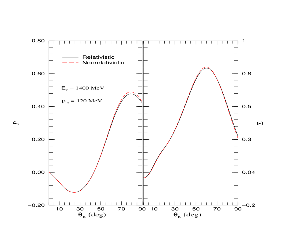
Figure 1: Comparison between relativistic and nonrelativistic calculations of the recoil polarization of the $\Lambda$-hyperon (${\cal P}$) and the photon asymmetry ($\Sigma$) as a function of the kaon scattering angle for the knockout of a proton from the $p^{3/2}$ orbital in ¹²C. The SL model for the elementary amplitude is used here.

$\Lambda-$hyperon and the photon asymmetry ($\Sigma$) as a function of the kaon scattering angle for the knockout of a proton from the $p^{3/2}$ orbital in ¹²C using the SL model for the elementary amplitude. The polarization observables were evaluated at a photon energy of $E_{\gamma}\!=\!1400$ MeV and at a missing momentum of $p_{m}\!=\!120$ MeV (this value is close to the maximum in the momentum distribution of the $p^{3/2}$ orbital; see Figure 3). Note that in this figure — and all throughout this chapter — we compute all observables in the laboratory system using the quasifree condition: $\omega\!=\!\sqrt{q^{2}+M_{\Lambda}^{2}}-M_{N}$. The insensitivity of our results to the relativistic dynamics is evident. Indeed, the relativistic and nonrelativistic curves can barely be resolved in the figure. We have also examined in Figure 2 these effects on the unpolarized cross

Figure 2: Comparison between relativistic and nonrelativistic calculations of the differential cross section as a function of the kaon scattering angle for the knockout of a proton from the $p^{3/2}$ orbital in ¹²C. The SL model for the elementary amplitude is used here.

section and found them insignificant as well. The main reason behind this insensitivity is that in the quasifree process all CGLN amplitudes including the tensor, pseudoscalar, and axialvector contributions participate in the process as opposed to the tensor one only (which is very sensitive to the relativistic enhancement) in the coherent process. Note that our “nonrelativistic” results were obtained by adopting the free-space relation in the determination of the lower-component of the bound-state wavefunction. This represents our best attempt at reproducing nonrelativistic calculations, which employ free, on-shell spinors to effect the nonrelativistic reduction of the elementary amplitude.

2 Nuclear Target Effects

Next we examine the nuclear dependence of the polarization observables. Figure 3 displays the recoil polarization and the

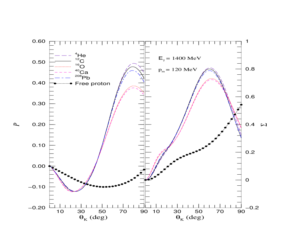
Figure 3: The recoil polarization of the $\Lambda$-hyperon (${\cal P}$) and the photon asymmetry ($\Sigma$) as a function of the kaon scattering angle for the knockout of a valence proton from a variety of nuclei. The photoproduction from a free proton is depicted with the filled circles. The SL model for the elementary amplitude is used here.

photon asymmetry for the knockout of a valence proton for a variety of nuclei, ranging from ⁴He all the way to ²⁰⁸Pb. That is, we have computed the knockout from the $1s^{1/2}$ orbital of ⁴He, the $1p^{3/2}$ orbital of ¹²C, the $1p^{1/2}$ orbital of ¹⁶O, the $1d^{3/2}$ orbital of ⁴⁰Ca, and the $3s^{1/2}$ orbital of ²⁰⁸Pb. We have included also polarization observables from a single free proton to establish a baseline for comparison against our bound–nucleon calculations. The sensitivity of the polarization observables to the nuclear target is rather small. Indeed, it seems that as soon as the quasifree process takes place from a proton bound to a “lump” of nuclear matter, the polarization observables become largely insensitive to the fine details of the lump. In other words, the polarization observables are not sensitive to the fine details of the bound-nucleon wavefunction. Moreover, the deviations from the free value (shown with the filled circles) are significant. This indicates important modifications to the elementary process in the nuclear medium.

3 Sensitivity to the Elementary Amplitude

Having established the independence of polarization observables to relativistic effects and to a large extent to the nuclear target, we are now in a good position to discuss the sensitivity of these observables to the elementary amplitude (note that an insensitivity of polarization observables to final-state interactions has been shown specifically for the kaon quasifree process in Ref. [25]). We display in Figure 4 the differential

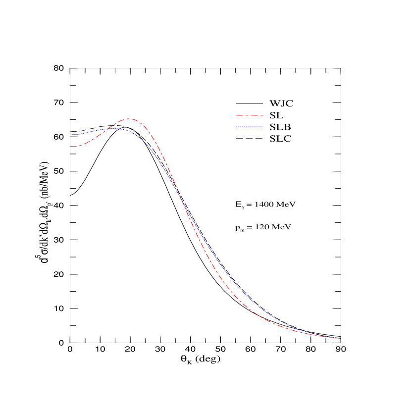
Figure 4: The differential cross section as a function of the kaon scattering angle for the knockout of a proton from the $p^{3/2}$ orbital in ¹²C using various models for the elementary amplitude.

cross section as a function of the kaon scattering angle for the knockout of a proton from the $p^{3/2}$ orbital in ¹²C using four different models for the elementary amplitude (see Section 3). Again, the photon incident energy and the missing momentum have been fixed at $1400$ MeV and $120$ MeV, respectively. Although there are noticeable differences between the models, primarily at small angles, these differences are relatively small. This behavior has been confirmed by a recent calculation that suggests that the kaon-photoproduction cross section — as a function of the energy of the photon beam — is slightly model dependent [63]. Much more significant, however, are the differences between the various sets for the case of the polarization observables displayed in Figure 5. The added

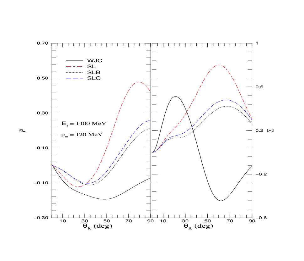
Figure 5: The recoil polarization of the $\Lambda$-hyperon (${\cal P}$) and the photon asymmetry ($\Sigma$) as functions of the kaon scattering angle for the knockout of a proton from the $p^{3/2}$ orbital in ¹²C using various models for the elementary amplitude.

sensitivity to the choice of amplitude exhibited by the polarization observables should not come as a surprise; unraveling subtle details about the dynamics is the hallmark of polarization observables. In particular, polarization observables show a strong sensitivity to the inclusion of the off-shell treatment for the various high-spin resonances, as suggested in Ref. [36]

4 Observables and Momentum Distribution in the Bound Nucleon Wavefunction

We display in Figure 6 the cross section as a function

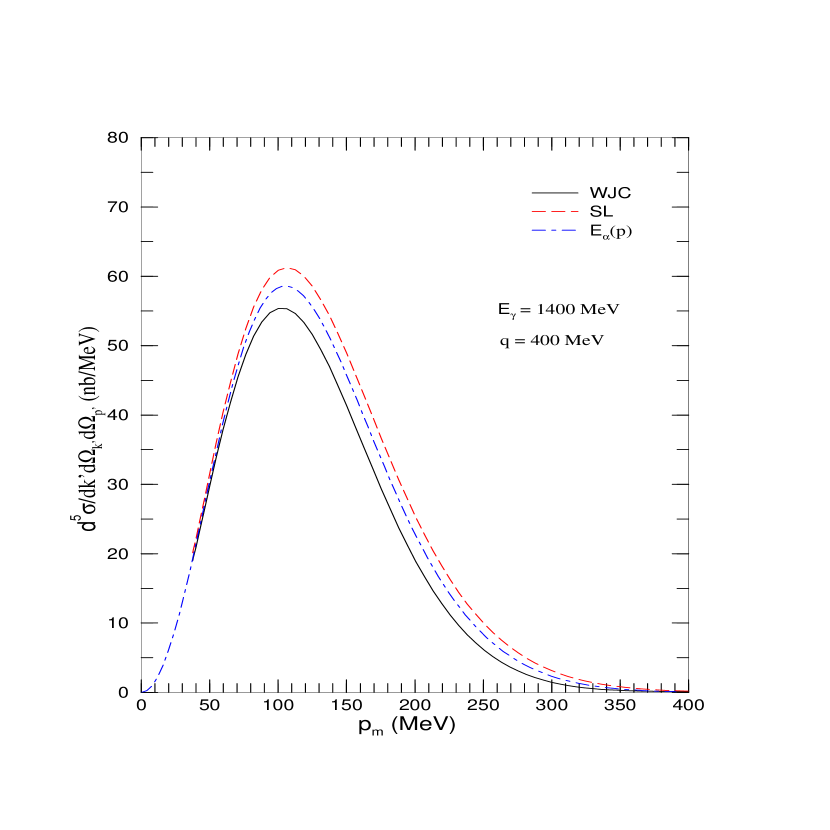
Figure 6: The differential cross section as a function of the missing momentum for the knockout of a proton from the $p^{3/2}$ orbital of ¹²C using two parameterizations of the elementary amplitude. The figure includes also the $E_{\alpha}$ parameter (up to an arbitrary scale) which is proportional to the momentum distribution of the bound-proton wavefunction.

of the missing momentum for the $p^{3/2}$ orbital in ¹²C using a different kinematical setting. Here we have kept the photon incident energy fixed at $1400$ MeV but have set the momentum transfer $q$ at $400$ MeV. To a large extent the cross sections represents — up to an overall normalization factor — the momentum distribution of the $p^{3/2}$ orbital. Indeed, the peak in the cross section is located at $p_{m}\!\approx\!110$ MeV, which is also the position of the maximum in the momentum distribution. To further appreciate the similarities between the two we have included the energy-like parameter $E_{\alpha}$, up to an arbitrary scale. As seen from Equation 23, $E_{\alpha}$ is directly proportional to the momentum distribution of the bound-proton wavefunction. The similarities between the cross section and the momentum distribution are indisputable. Note that the cross section dies out for $p_{\rm m}\!>\!250$ MeV. This region of high-momentum components is sensitive to short-range correlations, which are beyond the scope of our simple mean-field description. Thus, the tail of the photoproduction cross section can be used to test more sophisticated models of nuclear structure.

The sensitivity of the cross section to the momentum content in the bound-nucleon wavefunction suggests an innovative use for quasifree processes (although not using kaon photoproduction): probing neutron densities in halo nuclei. Halo nuclei are neutron-saturated nuclei where the valence neutrons (called also halo neutrons) are barely bound in the nucleus. Nuclear densities are usually studied using electron scattering which is a very clean tool, but one that discriminates against the neutrally charged neutron. Generally speaking, in meson photoproduction processes, the photon couples with comparable strengths to the protons and neutrons. Thus, the quasifree process is a direct tool for probing the neutron wavefunction in halo nuclei. This aspect is particularly appealing because the quasifree cross section is typically large enough to be measured experimentally, and there is a wealth of observables (such as polarization observables) to study. Furthermore, the process is only sensitive to the wavefunction of the knocked-out neutron, that is the process is minimally polluted by the other constituents in the nucleus. However, we cannot be ambitious to probe the fine details of the neutron wavefunction using this process. Studying halo nuclei using the quasifree process may encounter an experimental challenge as most of these nuclei have two halo neutrons and probably it is difficult to knock out only one of these neutrons without affecting the other; considering the fragility of the binding.

For completeness, Figure 7 displays the polarization observables

Figure 7: The recoil polarization of the $\Lambda$-hyperon (${\cal P}$) and the photon asymmetry ($\Sigma$) as functions of the missing momentum for the knockout of a proton from the $p^{3/2}$ orbital of ¹²C using two parameterizations of the elementary amplitude.

as functions of the missing momentum. The sensitivity of these observables to the elementary amplitude is manifest in the figure. It is notable however that these observables have a small magnitude and are rather insensitive to changes in the missing momentum. The evident sensitivity at larger values of the missing momentum is not to be taken seriously; the cross section at these values is too small for the ratios defining the polarization observables to be meaningful (see Equations 5 and 6).

Chapter 9 Conclusions of the Quasifree Process

We have computed polarization observables — the recoil polarization of the $\Lambda$-hyperon and the photon asymmetry — for the quasifree $K^{+}$ photoproduction reaction from nuclei [6]. Motivated by the large insensitivity of polarization observables to distortion effects, a relativistic plane-wave impulse approximation was developed. For the elementary amplitude we used a variety of models while for the nuclear structure we employed a relativistic mean-field approximation to the Walecka model [17]. In this manner the quasifree amplitude was evaluated without recourse to a nonrelativistic reduction, as the full relativistic structure of the amplitude was maintained.

By assuming the validity of the relativistic plane-wave impulse approximation an enormous simplification ensued: by introducing the notion of a bound-state propagator — as was done for the first time by Gardner and Piekarewicz in Ref. [26] — the mathematical structure of all quasifree observables was cast in a manner analogous to that of the elementary process. Thus, we brought the full power of Feynman’s trace techniques to bear into the problem. We stress that the relativistic formalism presented here can be applied with minor modifications to most quasifree knockout studies, at least in the plane-wave limit. In particular, the application of this formalism carries a prominent promise in the study of the quasifree processes of other pseudoscalar mesons like $\pi$ and $\eta$ mesons, as well as its use in quasifree electron scattering. Furthermore, the appropriateness of this process in probing neutron densities in halo nuclei is appealing.

In addition of being largely insensitive to distortions effects, we found polarization observables insensitive to relativistic effects and mostly independent of the target nucleus. Polarization observables appear to only be sensitive to the elementary amplitude. As free polarization observables provide a baseline against which possible medium effects may be inferred, we conclude that quasifree polarization observables might be one of the cleanest tools for probing modifications to the elementary amplitude in the nuclear medium. Deviations from their free values are likely to stem from a modification of the elementary interaction inside the nuclear medium due, for example, to a change in resonance parameters. Indeed, for the kinematics adopted in this work ($E_{\gamma}\!=\!1.4$ GeV or $\sqrt{s}\!\approx\!1.9$ GeV) one should be very sensitive to the formation, propagation, and decay of the $P_{13}(1900)$ and $F_{17}(1990)$ $N^{\star}-$resonances [64]. The meson photoproduction (and electroproduction) programs at various experimental facilities — such as TJNAF, NIKHEF, and MAMI — should shed light on the physics of this interesting and fundamental problem.

Shortly after submitting our work on the quasifree photoproduction for publication [6], a comprehensive study of kaon-photoproduction observables was reported by Lee, Mart, Bennhold, and Wright [65]. The authors have presented a very detailed analysis of the effect of distortions on various photoproduction observables. One of the central results from their study is that polarization observables are not as insensitive to distortion effects as once believed. Yet they showed categorically that for certain kinematical situations — such as those adopted in our present work — the effect of distortions on the polarization observables is insignificant indeed.

Chapter 10 General Conclusions

This manuscript presents the core of our studies in the field of pseudoscalar meson photoproduction from nuclei. We studied two processes: the coherent and the quasifree reactions. We have found that the current treatments of this process suffer from various sources of ambiguities and uncertainties. Among these problems are final-state interactions, relativistic effects, off-shell ambiguities, and violations to the impulse approximation. By far the largest uncertainty emerges from the ambiguity in extending the many on-shell-equivalent representations of the elementary amplitude off the mass shell. Thus one must be very cautious in interpreting the wealth of experimental data that will be available soon.

The coherent process can be a very useful tool in investigating nucleon resonances and their modifications in nuclear medium. In order to do so, the difficulties in this process must be addressed. Much work remains to be done in investigating the off-shell ambiguities and the violations to the impulse approximation. Developing a formalism that addresses all of these intricacies not only will help us understand these processes, but may have significant impact on our understanding of quantum chromodynamics (QCD) and its implicit symmetries. An example in this line of thought is our recent attempt to use the coherent eta photoproduction process as a probe of the chiral symmetry mirror assignment [66].

As for the quasifree process, we have developed a powerful formalism for studying these processes, at least in the plane-wave limit. We found that the most useful tools are the the polarization observables which are mostly insensitive to distortion, nuclear target, and relativistic effects. However, these observables are very sensitive to the fundamental physics behind the elementary process and to any modification in the nuclear medium. Thus, we have powerful tools at our disposal to study such aspects of photoproduction processes.

The quasifree formalism that we developed can be easily extended to studies of the quasifree processes of other mesons like the eta or the pion. In fact, we plan to embark on such a study. Furthermore, the formalism can be easily extended to electron-scattering quasifree processes and we plan also to study such processes. Finally, the most exciting is the study of the possibility of kaon condensation. This is done by investigating the inclusive kaon photoproduction from nuclei. This can be done using the single-particle response or the random-phase-approximation (RPA) response. Comparison of the theoretical results with expected experimental data may lead us to find a signature for this condensation.

Chapter 11 Generalized Calculations of Traces of $\gamma$-Matrices

As has been indicated in Chapter 7, the calculation of the square of the scattering matrix element reduces to a calculation of traces of $\gamma$-matrices in the free and quasifree processes. In this appendix, I include full calculations of the traces of $\gamma$-matrices for the generalized case involving two fermions, one of which is unpolarized with the propagator:

$$S_{\rm unpolarized}(p)\equiv\sum_{s}{\cal U}({\bf p},s)\,\overline{{\cal U}}({\bf p},s)=\frac{\hbox to0.0pt{/\hss}p+M}{2M}\;;\quad\left(p^{0}\equiv E({\bf p})=\sqrt{{\bf p}^{2}+M^{2}}\right),$$ (1)

while the other is polarized leading to the propagator:

$$S_{\rm polarized}\equiv{\cal U}({\bf p},s)\,\overline{{\cal U}}({\bf p},s)=\frac{\hbox to0.0pt{/\hss}p+M}{2M}\;\frac{1}{2}\;(1+\gamma^{5}\hbox to0.0pt{/\hss}s)\;;\quad\left(p^{0}\equiv E({\bf p})=\sqrt{{\bf p}^{2}+M^{2}}\right).$$ (2)

Hence, we can write the generalized structure of the traces as following:

$$Tr\left[\;\{{\cal L}\}\;(\hbox to0.0pt{/\hss}p_{1}+m_{1})\;\{{\cal R}\}\;(\hbox to0.0pt{/\hss}p_{2}+m_{2})\;\frac{1}{2}\;(1+\hbox to0.0pt{/\hss}s_{2}\gamma^{5})\;\right],$$ (3)

where ${p_{1}}$ is the four-momentum of the unpolarized fermion, ${p_{2}}$ is the four-momentum of the polarized one, whereas ${s_{2}}$ is the negative of the four-spin of the polarized fermion. The author apologizes for this awkward definition of the spin, but this has to do with the “history” of writing this appendix.

In this algebraic structure, ${\cal L}$ can be any item of the set

$$\{{\cal L}\}\equiv\{{1,\gamma^{\mu},\gamma^{\mu}\gamma^{5},i\gamma^{5},\sigma^{\mu\nu}}\}\;,$$ (4)

while ${\cal R}$ can be any item of the set

$$\{{\cal R}\}\equiv\{{1,\gamma^{\alpha},\gamma^{\alpha}\gamma^{5},i\gamma^{5},\sigma^{\alpha\beta}}\}\;.$$ (5)

The item $\sigma^{\delta\rho}$ in the above sets is defined as

$$\sigma^{\delta\rho}\equiv\frac{i}{2}[\gamma^{\delta},\gamma^{\rho}]\;.$$ (6)

The symbolic calculations of these traces have been achieved using FeynCalc 1.0[62] package of Mathematica 2.0. The package has been written by Mertig and Hubland specifically for high-energy physics calculations. The results of the analysis are shown in the following five tables. Each table corresponds to one item of the set $\{{\cal L}\}$ with each item of the set $\{{\cal R}\}$.

Table 1: ${1}$

	$1$
$1$	$2m_{1}m_{2}+2p_{1}.p_{2}$
$\gamma^{\alpha}$	$-2i\varepsilon^{\alpha\gamma\delta\rho}{p_{1}}_{\gamma}{p_{2}}_{\delta}{s_{2}}_{\rho}+2m_{2}{p_{1}}^{\alpha}+2m_{1}{p_{2}}^{\alpha}$
$\gamma^{\alpha}\gamma^{5}$	$-2p_{2}.s_{2}{p_{1}}^{\alpha}+2p_{1}.s_{2}{p_{2}}^{\alpha}-2m_{1}m_{2}{s_{2}}^{\alpha}-2p_{1}.p_{2}{s_{2}}^{\alpha}$
$i\gamma^{5}$	$2im_{2}p_{1}.s_{2}+2im_{1}p_{2}.s_{2}$
$\sigma^{\alpha\beta}$	$2m_{2}\varepsilon^{\alpha\beta\delta\rho}{p_{1}}_{\delta}{s_{2}}_{\rho}+2m_{1}\varepsilon^{\alpha\beta\delta\rho}{p_{2}}_{\delta}{s_{2}}_{\rho}+2i{p_{1}}^{\beta}{p_{2}}^{\alpha}-2i{p_{1}}^{\alpha}{p_{2}}^{\beta}$

Table 2: $\gamma^{\mu}$

	$\gamma^{\mu}$
$1$	$2i\varepsilon^{\mu\gamma\delta\rho}{p_{1}}_{\gamma}{p_{2}}_{\delta}{s_{2}}_{\rho}+2m_{2}{p_{1}}^{\mu}+2m_{1}{p_{2}}^{\mu}$
$\gamma^{\alpha}$	$2im_{2}\varepsilon^{\alpha\mu\delta\rho}{p_{1}}_{\delta}{s_{2}}_{\rho}-2im_{1}\varepsilon^{\alpha\mu\delta\rho}{p_{2}}_{\delta}{s_{2}}_{\rho}+2m_{1}m_{2}g^{\alpha\mu}$
	$-2g^{\alpha\mu}p_{1}.p_{2}+2{p_{1}}^{\mu}{p_{2}}^{\alpha}+2{p_{1}}^{\alpha}{p_{2}}^{\mu}$
$\gamma^{\alpha}\gamma^{5}$	$-2i\varepsilon^{\alpha\mu\delta\rho}{p_{1}}_{\delta}{p_{2}}_{\rho}+2m_{2}g^{\alpha\mu}p_{1}.s_{2}-2m_{1}g^{\alpha\mu}p_{2}.s_{2}+2m_{2}{p_{1}}^{\mu}{s_{2}}^{\alpha}$
	$-2m_{1}{p_{2}}^{\mu}{s_{2}}^{\alpha}-2m_{2}{p_{1}}^{\alpha}{s_{2}}^{\mu}+2m_{1}{p_{2}}^{\alpha}{s_{2}}^{\mu}$
$i\gamma^{5}$	$2ip_{2}.s_{2}{p_{1}}^{\mu}+2ip_{1}.s_{2}{p_{2}}^{\mu}+2im_{2}m_{1}{s_{2}}^{\mu}-2ip_{1}.p_{2}{s_{2}}^{\mu}$
$\sigma^{\alpha\beta}$	$2m_{1}m_{2}\varepsilon^{\alpha\beta\mu\rho}{s_{2}}_{\rho}+2\varepsilon^{\alpha\beta\mu\rho}{p_{1}}_{\rho}p_{2}.s_{2}-2\varepsilon^{\beta\mu\delta\rho}{p_{2}}_{\delta}{s_{2}}_{\rho}{p_{1}}^{\alpha}$
	$-2im_{2}g^{\beta\mu}{p_{1}}^{\alpha}+2\varepsilon^{\alpha\mu\delta\rho}{p_{2}}_{\delta}{s_{2}}_{\rho}{p_{1}}^{\beta}+2im_{2}g^{\alpha\mu}{p_{1}}^{\beta}$
	$+2im_{1}g^{\beta\mu}{p_{2}}^{\alpha}-2im_{1}g^{\alpha\mu}{p_{2}}^{\beta}+2\varepsilon^{\alpha\beta\delta\rho}{p_{1}}_{\delta}{s_{2}}_{\rho}{p_{2}}^{\mu}$

Table 3: $\gamma^{\mu}\gamma^{5}$

	$\gamma^{\mu}\gamma^{5}$
$1$	$2p_{2}.s_{2}{p_{1}}^{\mu}+2p_{1}.s_{2}{p_{2}}^{\mu}-2m_{1}m_{2}{s_{2}}^{\mu}-2p_{1}.p_{2}{s_{2}}^{\mu}$
$\gamma^{\alpha}$	$-2i\varepsilon^{\alpha\mu\delta\rho}{p_{1}}_{\delta}{p_{2}}_{\rho}+2m_{2}g^{\alpha\mu}p_{1}.s_{2}+2m_{1}g^{\alpha\mu}p_{2}.s_{2}-2m_{2}{p_{1}}^{\mu}{s_{2}}^{\alpha}$
	$+2m_{1}{p_{2}}^{\mu}{s_{2}}^{\alpha}-2m_{2}{p_{1}}^{\alpha}{s_{2}}^{\mu}-2m_{1}{p_{2}}^{\alpha}{s_{2}}^{\mu}$
$\gamma^{\alpha}\gamma^{5}$	$2im_{2}\varepsilon^{\alpha\mu\delta\rho}{p_{1}}_{\delta}{s_{2}}_{\rho}+2im_{1}\varepsilon^{\alpha\mu\delta\rho}{p_{2}}_{\delta}{s_{2}}_{\rho}-2m_{1}m_{2}g^{\alpha\mu}$
	$-2g^{\alpha\mu}p_{1}.p_{2}+2{p_{1}}^{\mu}{p_{2}}^{\alpha}+2{p_{1}}^{\alpha}{p_{2}}^{\mu}$
$i\gamma^{5}$	$-2\varepsilon^{\mu\gamma\delta\rho}{p_{1}}_{\gamma}{p_{2}}_{\delta}{s_{2}}_{\rho}+2im_{2}{p_{1}}^{\mu}-2im_{1}{p_{2}}^{\mu}$
$\sigma^{\alpha\beta}$	$-2m_{2}\varepsilon^{\alpha\beta\mu\rho}{p_{1}}_{\rho}-2m_{1}\varepsilon^{\alpha\beta\mu\rho}{p_{2}}_{\rho}-2ig^{\beta\mu}p_{2}.s_{2}{p_{1}}^{\alpha}+2ig^{\alpha\mu}p_{2}.s_{2}{p_{1}}^{\beta}$
	$+2ig^{\beta\mu}p_{1}.s_{2}{p_{2}}^{\alpha}-2ig^{\alpha\mu}p_{1}.s_{2}{p_{2}}^{\beta}-2im_{1}m_{2}g^{\beta\mu}{s_{2}}^{\alpha}-2ig^{\beta\mu}p_{1}.p_{2}{s_{2}}^{\alpha}$
	$+2i{p_{1}}^{\mu}{p_{2}}^{\beta}{s_{2}}^{\alpha}+2i{p_{1}}^{\beta}{p_{2}}^{\mu}{s_{2}}^{\alpha}+2im_{1}m_{2}g^{\alpha\mu}{s_{2}}^{\beta}+2ig^{\alpha\mu}p_{1}.p_{2}{s_{2}}^{\beta}$
	$-2i{p_{1}}^{\mu}{p_{2}}^{\alpha}{s_{2}}^{\beta}-2i{p_{1}}^{\alpha}{p_{2}}^{\mu}{s_{2}}^{\beta}-2i{p_{1}}^{\beta}{p_{2}}^{\alpha}{s_{2}}^{\mu}+2i{p_{1}}^{\alpha}{p_{2}}^{\beta}{s_{2}}^{\mu}$

Table 4: $i\gamma^{5}$

	$i\gamma^{5}$
$1$	$-2im_{2}p_{1}.s_{2}+2im_{1}p_{2}.s_{2}$
$\gamma^{\alpha}$	$2ip_{2}.s_{2}{p_{1}}^{\alpha}-2ip_{1}.s_{2}{p_{2}}^{\alpha}+2i{s_{2}}^{\alpha}(p_{1}.p_{2}-m_{1}m_{2})$
$\gamma^{\alpha}\gamma^{5}$	$-2\varepsilon^{\alpha\gamma\delta\rho}{p_{1}}_{\gamma}{p_{2}}_{\delta}{s_{2}}_{\rho}-2im_{2}{p_{1}}^{\alpha}+2im_{1}{p_{2}}^{\alpha}$
$i\gamma^{5}$	$-2m_{1}m_{2}+2p_{1}.p_{2}$
$\sigma^{\alpha\beta}$	$-2i\varepsilon^{\alpha\beta\delta\rho}{p_{1}}_{\delta}{p_{2}}_{\rho}+2m_{2}{p_{1}}^{\beta}{s_{2}}^{\alpha}-2m_{1}{p_{2}}^{\beta}{s_{2}}^{\alpha}-2m_{2}{p_{1}}^{\alpha}{s_{2}}^{\beta}+2m_{1}{p_{2}}^{\alpha}{s_{2}}^{\beta}$

Table 5: $\sigma^{\mu\nu}$

	$\sigma^{\mu\nu}$
$1$	$2m_{2}\varepsilon^{\mu\nu\delta\rho}{p_{1}}_{\delta}{s_{2}}_{\rho}+2m_{1}\varepsilon^{\mu\nu\delta\rho}{p_{2}}_{\delta}{s_{2}}_{\rho}-2i{p_{1}}^{\nu}{p_{2}}^{\mu}+2i{p_{1}}^{\mu}{p_{2}}^{\nu}$
$\gamma^{\alpha}$	$2m_{1}m_{2}\varepsilon^{\alpha\mu\nu\rho}{s_{2}}_{\rho}+\varepsilon^{\nu\gamma\delta\rho}{p_{1}}_{\gamma}{p_{2}}_{\delta}{s_{2}}_{\rho}g^{\alpha\mu}-\varepsilon^{\mu\gamma\delta\rho}{p_{1}}_{\gamma}{p_{2}}_{\delta}{s_{2}}_{\rho}g^{\alpha\nu}-2\varepsilon^{\alpha\mu\nu\rho}{p_{1}}_{\rho}p_{2}.s_{2}$
	$+2\varepsilon^{\mu\nu\delta\rho}{p_{2}}_{\delta}{s_{2}}_{\rho}{p_{1}}^{\alpha}+\varepsilon^{\alpha\nu\delta\rho}{p_{2}}_{\delta}{s_{2}}_{\rho}{p_{1}}^{\mu}+2im_{2}g^{\alpha\nu}{p_{1}}^{\mu}$
	$-\varepsilon^{\alpha\mu\delta\rho}{p_{2}}_{\delta}{s_{2}}_{\rho}{p_{1}}^{\nu}-2im_{2}g^{\alpha\mu}{p_{1}}^{\nu}+\varepsilon^{\alpha\nu\delta\rho}{p_{1}}_{\delta}{s_{2}}_{\rho}{p_{2}}^{\mu}$
	$-2im_{1}g^{\alpha\nu}{p_{2}}^{\mu}-\varepsilon^{\alpha\mu\delta\rho}{p_{1}}_{\delta}{s_{2}}_{\rho}{p_{2}}^{\nu}+2im_{1}g^{\alpha\mu}{p_{2}}^{\nu}$
$\gamma^{\alpha}\gamma^{5}$	$-2m_{2}\varepsilon^{\alpha\mu\nu\rho}{p_{1}}_{\rho}-2m_{1}\varepsilon^{\alpha\mu\nu\rho}{p_{2}}_{\rho}-2ig^{\alpha\nu}p_{2}.s_{2}{p_{1}}^{\mu}+2ig^{\alpha\mu}p_{2}.s_{2}{p_{1}}^{\nu}$
	$-2ig^{\alpha\nu}p_{1}.s_{2}{p_{2}}^{\mu}+2ig^{\alpha\mu}p_{1}.s_{2}{p_{2}}^{\nu}+2i{p_{1}}^{\nu}{p_{2}}^{\mu}{s_{2}}^{\alpha}-2i{p_{1}}^{\mu}{p_{2}}^{\nu}{s_{2}}^{\alpha}$
	$+2im_{1}m_{2}g^{\alpha\nu}{s_{2}}^{\mu}+2ig^{\alpha\nu}p_{1}.p_{2}{s_{2}}^{\mu}-2i{p_{1}}^{\nu}{p_{2}}^{\alpha}{s_{2}}^{\mu}-2i{p_{1}}^{\alpha}{p_{2}}^{\nu}{s_{2}}^{\mu}$
	$-2im_{1}m_{2}g^{\alpha\mu}{s_{2}}^{\nu}-2ig^{\alpha\mu}p_{1}.p_{2}{s_{2}}^{\nu}+2i{p_{1}}^{\mu}{p_{2}}^{\alpha}{s_{2}}^{\nu}+2i{p_{1}}^{\alpha}{p_{2}}^{\mu}{s_{2}}^{\nu}$
$i\gamma^{5}$	$2i\varepsilon^{\mu\nu\delta\rho}{p_{1}}_{\delta}{p_{2}}_{\rho}+2m_{2}{p_{1}}^{\nu}{s_{2}}^{\mu}-2m_{1}{p_{2}}^{\nu}{s_{2}}^{\mu}-2m_{2}{p_{1}}^{\mu}{s_{2}}^{\nu}+2m_{1}{p_{2}}^{\mu}{s_{2}}^{\nu}$
$\sigma^{\alpha\beta}$	$-im_{1}\varepsilon^{\beta\nu\delta\rho}{p_{2}}_{\delta}{s_{2}}_{\rho}g^{\alpha\mu}+im_{1}\varepsilon^{\beta\mu\delta\rho}{p_{2}}_{\delta}{s_{2}}_{\rho}g^{\alpha\nu}+im_{1}\varepsilon^{\alpha\nu\delta\rho}{p_{2}}_{\delta}{s_{2}}_{\rho}g^{\beta\mu}-2m_{1}m_{2}g^{\alpha\nu}g^{\beta\mu}$
	$-im_{1}\varepsilon^{\alpha\mu\delta\rho}{p_{2}}_{\delta}{s_{2}}_{\rho}g^{\beta\nu}+2m_{1}m_{2}g^{\alpha\mu}g^{\beta\nu}-2g^{\alpha\nu}g^{\beta\mu}p_{1}.p_{2}+2g^{\alpha\mu}g^{\beta\nu}p_{1}.p_{2}$
	$-2im_{1}\varepsilon^{\alpha\beta\mu\nu}p_{2}.s_{2}-2im_{2}\varepsilon^{\beta\mu\nu\rho}{s_{2}}_{\rho}{p_{1}}^{\alpha}+2im_{2}\varepsilon^{\alpha\mu\nu\rho}{s_{2}}_{\rho}{p_{1}}^{\beta}-2g^{\beta\nu}{p_{1}}^{\mu}{p_{2}}^{\alpha}$
	$+2g^{\beta\mu}{p_{1}}^{\nu}{p_{2}}^{\alpha}+2g^{\alpha\nu}{p_{1}}^{\mu}{p_{2}}^{\beta}-2g^{\alpha\mu}{p_{1}}^{\nu}{p_{2}}^{\beta}-im_{1}\varepsilon^{\alpha\beta\nu\rho}{s_{2}}_{\rho}{p_{2}}^{\mu}$
	$-2g^{\beta\nu}{p_{1}}^{\alpha}{p_{2}}^{\mu}+2g^{\alpha\nu}{p_{1}}^{\beta}{p_{2}}^{\mu}+im_{1}\varepsilon^{\alpha\beta\mu\rho}{s_{2}}_{\rho}{p_{2}}^{\nu}+2g^{\beta\mu}{p_{1}}^{\alpha}{p_{2}}^{\nu}$
	$-2g^{\alpha\mu}{p_{1}}^{\beta}{p_{2}}^{\nu}-im_{2}\varepsilon^{\alpha\beta\nu\rho}{p_{1}}_{\rho}{s_{2}}^{\mu}+im_{2}\varepsilon^{\alpha\beta\mu\rho}{p_{1}}_{\rho}{s_{2}}^{\nu}$

Personal
Date of Birth: June 3, 1970. Place of Birth: Amman, Jordan. Marital Status: Married, with one son. Languages: Arabic and English; limited Spanish. Nationality: Jordanian. Immigration Status: Permanent resident of the U.S.A.

Education
2000 Ph.D. in physics, specialization in computational theoretical nuclear physics, Florida State University. G.P.A. 4.0.
Dissertation: “Photoproduction of Pseudoscalar Mesons from Nuclei”. 1994 M.Sc. in physics, specialization in experimental condensed matter physics, Miami University. G.P.A. 4.0.
Thesis: “Perturbed Angular Correlation Spectroscopy Study of the Recrystallization of Natural Zircon”. 1992 B.Sc. in physics, University of Jordan. G.P.A. 90.4 %.

Experience
2000 to present Postdoctoral Research Associate, School of Computational Science and Information Technology (CSIT), Florida State University. 1995 to 2000 Research Assistant, School of Computational Science and Information Technology (CSIT), Florida State University. July 97 Research Assistant, Thomas Jefferson National Accelerator Facility (TJNAF). 1994 to 1995 Teaching Assistant, Department of Physics, Florida State University. 1992 to 1994 Teaching Assistant, Department of Physics, Miami University.

Honors and Awards
April 2000 Dirac-Hellmann Award in Theoretical Physics, Florida State University. June to August 1999 Summer Institute in Japan Fellowship, National Science Foundation (NSF) and Science and Technology Agency of Japan (STA). 1996 to 1998 SURA/Jefferson Laboratory Fellowship, Thomas Jefferson National Accelerator Facility (TJNAF). August 1997 Ninth Annual Summer School in Nuclear Physics Scholarship, Yale University. June 1996 HUGS at Jefferson Laboratory Fellowship, Thomas Jefferson National Accelerator Facility (TJNAF). July 1992 Ranked first in the B.Sc. degree, University of Jordan. Member of $\Sigma\Pi\Sigma$ and $\Phi K\Phi$ honor societies.

Analytical and Computational Skills

Analytical Skills:

Scientific research using various aspects of applied mathematics such as mathematical simulation and modeling, numerical analysis, differential and integral equations, Green’s functions and boundary value problems, group theory, calculus of variation, variational methods, and perturbation theory.

Computational Skills

: Scientific computing involving programming, symbolic and logical analysis, Monte Carlo simulations, algorithm development, data analysis, and software development.

• Programming Languages: FORTRAN and C⁺⁺.

• Symbolic Manipulators: Mathematica and Maple.

• Operating Systems: UNIX.
  

General Research Interests
Theoretical nuclear physics, mathematical physics, and computational physics.

Ph.D. Dissertation Advisor
Jorge Piekarewicz at Florida State University.

Additional Research Advisors
Makoto Oka at Tokyo Institute of Technology during the NSF Summer Institute in Japan Fellowship.
José Goity at Thomas Jefferson National Accelerator Facility (TJNAF) and Hampton University during the research assistantship at Jefferson Laboratory.

Publications

1. L.J. Abu-Raddad and J. Piekarewicz, “Quasifree kaon photoproduction from nuclei in a relativistic approach”, Phys. Rev. C (61), 014604, (2000).

2. L.J. Abu-Raddad, J. Piekarewicz, A.J. Sarty, and R.A. Rego, “Lessons to be learned from the coherent photoproduction of pseudoscalar mesons”, Phys. Rev. C (60), 054606 (1999).

3. L.J. Abu-Raddad, J. Piekarewicz, A.J. Sarty, and M. Benmerrouche, “Nuclear dependence of the coherent $\eta$ photoproduction reaction in a relativistic approach”, Phys. Rev. C (57), 2053 (1998).

4. H. Jaeger, L.J. Aburaddad, and D. Wick, “TDPAC study of structural disorder in metamict zircon”, App. Radiat. Isotopes 48 (8), 1083 (1997).

5. L. Abu-Raddad, R. Klindworth, and L. Zhang, “Two theories of baryons”, Proceedings of the 11th HUGS at CEBAF Workshop, 22 (1996).

6. H. Jaeger, L.J. Aburaddad, “Two-detector coincidence routing circuit for personal computer-based multichannel analyzer”, Rev. Sci. Intrum. 66 (4), 3069 (1995).

Presentations and Conferences

1. L.J. Abu-Raddad, “Photoproduction of pseudoscalar mesons from nuclei”, TRIUMF, February 2000, Vancouver, Canada.

2. L.J. Abu-Raddad and J. Piekarewicz, “Quasifree kaon photoproduction from nuclei in a relativistic approach”, Fall Meeting of the Division of Nuclear Physics of the American Physical Society, October 1999, Asilomar, California.

3. L.J. Abu-Raddad, “Photoproduction of pseudoscalar mesons from nuclei”, presented at the July Mini Workshop, Tokyo Institute of Technology, July 1999, Tokyo, Japan. It has been also presented at the Research Center for Nuclear Physics (RCNP), August 1999, Osaka University, Osaka, Japan, and at the Department of Physics, Osaka City University, August 1999, Osaka, Japan.

4. L.J. Abu-Raddad, J. Piekarewicz, and A.J. Sarty, “Coherent photoproduction of neutral pions”, Centennial Meeting of the American Physical Society, March 1999, Atlanta, Georgia.

5. L.J. Abu-Raddad, J. Piekarewicz, A.J. Sarty, and M. Benmerrouche, “Nuclear dependence of the coherent $\eta$ photoproduction of from nuclei”, Fall Meeting of the Division of Nuclear Physics of the American Physical Society, October 1997, Whistler, Canada.

6. L.J. Abu-Raddad and H. Jaeger, “TDPAC study of natural zircon”, Spring Meeting of the Ohio Section of the American Physical Society, May 1994, Cleveland, Ohio.

References

- [1] WWWWebster Dictionary, World Wide Web, http://www.m-w.com/cgi-bin/dictionary.
- [2] J. Piekarewicz, A. J. Sarty, and M. Benmerrouche, Phys. Rev. C 55, 2571 (1997).