Neutrino-pair emission in a strong magnetic field

Abstract

We study the neutrino emissivity of strongly magnetized neutron stars due to the charged and neutral current couplings of neutrinos to baryons in strong magnetic fields. The leading order neutral current process is the one-body neutrino-pair bremsstrahlung, which does not have an analogue in the zero field limit. The leading order charged current reaction is the known generalization of the direct Urca processes to strong magnetic fields. While for superstrong magnetic fields in excess of $10^{18}$ G the direct Urca process dominates the one-body bremsstrahlung, we find that for fields on the order $10^{16}-10^{17}$ G and temperatures a few times $10^{9}$ K the one-body bremsstrahlung is the dominant process. Numerical computation of the resulting emissivity, based on a simple parametrization of the equation of state of the $npe$-matter in a strong magnetic field, shows that the emissivity of this reaction is of the same order of magnitude as that of the modified Urca process in the zero field limit.

1 Introduction

It is now well established that the neutron stars which are observed as radio-pulsars posses $B$-fields of the order of $10^{12}$-$10^{13}$ G at the surface. The interior fields are unknown, but can be by several orders of magnitude larger than the ones inferred for the surface. The scalar virial theorem sets an upper limit on the magnetic field strength of a neutron star of the order of $10^{18}\rm{G}$ (Lai & Shapiro Lai (1991)). Similar conclusion is reached through more sophisticated numerical studies (Bocquet et al. Boc (1995)).

Recent measurements of the spin-down timescales of several soft gamma-ray repeaters, such as SGR 0526-66 (Mazets et al. Maz (1979)), SGR 1806-20 (Murakami et al. Mur (1994)), and SGR 1900+14 (Kouveliotou et al. Kou1 (1998)) with RXTE, ASCA and BeppoSAX have made a strong case for SGRs as being newly born neutron stars that have very large surface magnetic fields (up to $10^{15}$ G). The subsequent discoveries of the SGR 1627-41 by BATSE (Woods et al. Woods (1999)) and SGR 1801-23 by Ulysses, BATSE, and KONUS-Wind (Cline et al. Cline (1999)) lent further support to the identification of SGRs with highly magnetized neutron stars. These objects were naturally related to the magnetars, which are thought to be remnants of a supernova explosion which develop high magnetic fields via a dynamo mechanism (Duncan & Thompson Dun (1992), Thompson & Duncan Thom (1995)). The magnetars also serve as a model for the anomalous X-ray pulsars (AXP) (van Paradijs, Taam & van den Heuvel Para (1995)) such as 1E 1841-045 (Kes 73) (Gotthelf, Vasisht, & Dotani Gott (1999)), RX J0720.4-3125 (Haberl et al. Hab (1997)), and 1E 2259+586 (Rho & Petre Rho (1997)).

Neutrino-nucleon interactions in the strong magnetic fields have been studied recently both in the supernova and neutron star contexts. It has been pointed out that the neutrino emission from proto-neutron stars, which is anisotropic in strong $B$-fields, could produce the “pulsar kicks” if the fields are in excess of $10^{16}$ G (Horowitz & Li Horo (1998); Arras & Lai Arras (1999) and references therein). The strong magnetic fields relax the kinematical constrains on the direct Urca process and hence give rise to finite neutrino emissivity even when the proton fraction is small (Leinson & Perez Leinson (1998), Bandyopadhyay et al. Band (1998)). The effect is most pronounced in the ultra-high magnetic fields when protons and the electrons occupy the lowest Landau levels. The direct Urca process for arbitrary magnetic fields, when the protons and electrons are allowed to occupy many Landau levels, has also been studied (Baiko & Yakovlev Baiko (1999)).

The neutrino emissivities via the one-body processes sensitively depend on the abundances of the various species of baryons and leptons which are controlled by the equation of state (EoS) of the dense matter in strong magnetic fields. The strong magnetic fields lead to an increase of the proton fraction (Broderick, Prakash & Lattimer Bro (2000)). The muon production and pion condensation in strong magnetic softens the EoS of the dense matter (Suh & Mathews Suh (1999)). For the purpose of estimating the magnitude of the neutrino emissivities, we employ in this paper a simple parametrization of the EoS for the $npe$-matter in strong magnetic fields.

The main objective of this paper is to show that the strong magnetic fields open a new channel of neutrino emission via one-body neutral current bremsstrahlung, which does not have an analogue in the zero field limit. We also briefly discuss the direct Urca process, which is forbidden in the low-density zero-field limit (as long as the triangular condition $p_{Fp}+p_{Fe}\geq p_{Fn}$ is not satisfied), but is allowed in strong magnetic fields because of the relaxation of the kinematical constrains. We compare the emissivities of various reactions using a simple parametrization of the EoS for the $npe$ matter in a strong $B$-field. As a standard reference for our comparison we use the modified Urca process. The presence of a magnetic field has two different effects on neutrino emissivities: (i) in pure neutron matter it allows for spin-flip transitions where the finite difference of the momenta of neutrons at two different Fermi surfaces enables one to satisfy energy-momentum conservation, (ii) the charged particles occupy Landau levels leading to a smearing of the transverse momenta over an amount $\sqrt{eB}$ . As a consequence there are two typical scales of the magnetic field, where effects on the emissivity are expected; first for $|\mu_{B}|B\sim T$ which is relevant in neutrino-pair bremsstrahlung from neutrons, and second $eB\sim p_{F}^{2}$ relevant for the Urca process.

As well know, the emissivity of any particular reaction can be related to the imaginary part of the polarization function of the medium (Voskresensky & Senatorov VS (1986), Raffelt & Seckel Raffelt (1995), Sedrakian & Dieperink Se1 (1999)). We compute the polarization function of neutrons and protons in strong magnetic fields employing the finite temperature Matsubara Green’s functions technique. For the case of the bremsstrahlung the time-like properties of the polarization function are relevant. The space-like properties of the polarization function, relevant for the neutrino-nucleon scattering, have been studied by Arras & Lai (Arras (1999)) in an equivalent response function formalism.

The plan of this paper is as follows. The bremsstrahlung emissivity is related to the polarization function of the medium in Sect. 2. The neutrino emissivity via neutrino-pair bremsstrahlung from neutrons is discussed in Sect. 3 and that from protons in Sect. 4. The Urca process in strong magnetic fields is briefly discussed Sect. 5. The EoS of $npe$ matter in a magnetic field is discussed in Sect. 6. Our numerical results are presented in Sect. 7. Sect. 8 contains our conclusions.

2 The bremsstrahlung emissivity

The neutrino emissivity of an infinite medium of interacting hadrons can be expressed in terms of the imaginary part of the finite temperature polarization function $\Pi(\@vec{q},\omega),$ where $\@vec{q}$ and $\omega$ denote the momentum and energy transfer to the leptons. In the single-loop approximation the finite temperature polarization function in a magnetic field is a 2 $\times$ 2 matrix in spin space (Mattuck Mat (1992))

$$\Pi_{s,s^{\prime}}(\@vec{q},\omega)=\frac{-2}{\beta}\int\frac{d^{3}p}{(2\pi)^{3}}\sum_{i(p+q)}G_{s^{\prime}}(\@vec{p}+\@vec{q},ip+iq)$$

$$G_{s}(\@vec{p},ip),$$ (1)

where $\beta$ is the inverse temperature. The single-particle Green function can be expressed as $G_{s}(\@vec{p},ip)=[ip-(E_{p,s}-E_{F})]^{-1}$, where $E_{F}$ is the Fermi energy and $ip$ is the Matsubara frequency; $s^{\prime},s=\pm 1$ specify the initial and final nucleon spins. (We assume the magnetic field along the positive $z-$axis.) Carrying out the frequency summation and taking the imaginary part one finds the well-known result (Mattuck Mat (1992))

$${\rm Im}\Pi_{s,s^{\prime}}(\@vec{q},\omega)=2\pi\int\frac{d^{3}p}{(2\pi)^{3}}(f(E_{p,s})-f(E_{p+q,s^{\prime}}))$$

$$\delta(E_{p,s}-E_{p+q,s^{\prime}}+\omega),$$ (2)

where $f(E_{p,s})=[e^{\beta(E{p,s}-E_{F})}+1]^{-1}$ is the Fermi-distribution function. The emissivity is then given by

$$\epsilon_{\nu\overline{\nu}}=3\sum_{ss^{\prime}}|M_{s,s^{\prime}}|^{2}\int\frac{d^{3}p_{\nu}}{(2\pi)^{3}}\frac{d^{3}p_{\overline{\nu}}}{(2\pi)^{3}}d\omega\,d^{3}q\,\,{\rm Im}\Pi_{s,s^{\prime}}(\@vec{q},\omega)$$

$$g_{B}(\omega)\,\omega\,\delta({\omega}-{\omega}_{\nu}-{\omega}_{\overline{\nu}})\,\delta^{3}(\@vec{q}-\@vec{p}_{\nu}-\@vec{p}_{\overline{\nu}}),$$ (3)

where $g_{B}(\omega)=[e^{\beta\omega}-1]^{-1}$ is the Bose distribution function, the factor 3 comes from the sum over the neutrino flavours, and the weak interaction matrix (neglecting lepton momenta) is $|M_{s,s^{\prime}}|^{2}=(G_{F}/2)^{2}(c^{2}_{V}\delta_{s,s^{\prime}}+c^{2}_{A}(2\delta_{s,-s^{\prime}}+\delta_{s,s^{\prime}}))$ with $c_{V}$ and $c_{A}$ the vector and axial vector coupling constants and $G_{F}$ the Fermi weak coupling constant (see Appendix B).

3 Neutrino-pair bremsstrahlung from neutrons  ($n\rightarrow n+\nu+\overline{\nu}$)

In the absence of a magnetic field the imaginary part of the polarization function vanishes for time-like processes in the quasi-particle approximation, because energy and momentum cannot be conserved simultaneously. In a pure neutron system a magnetic field $B$ will give rise to a difference between the Fermi momenta of the neutrons with spin parallel and spin anti-parallel to the $B$-field (see Appendix A)

$$p^{s}_{Fn}=(E^{2}_{Fn}-m^{2}-sg_{n}eB)^{1/2},$$

where $\mu_{n}=g_{n}e/(2m)$ is the neutron magnetic moment and $g_{n}=-1.91$ is the neutron $g$-factor and we assume $\mu_{n}B\ll m$. For $B\not=0$ energy-momentum conservation can be satisfied, and as a result one may expect that a field with strength $|\mu_{n}|B\sim T$ leads to a finite spin-flip polarization function whenever $\omega\sim|\mu_{n}|B$.

3.1 Polarization function

In the time-like region it is preferable to use the relativistic kinematics. The non-relativistic kinematics does not produce the correct zero-field limit $\Pi(\@vec{q},\omega,B=0)=0$, rather a spurious finite contribution $\Pi(\@vec{q},\omega,B=0)\propto\exp(-m/T)$. To evaluate the angular integral in eq. (2) note that the energy conserving $\delta$-function is non-zero if $|\cos(\theta_{pq})|\leq 1$, where $\theta_{pq}$ is the angle between the momentum vector $\@vec{p}$ of the neutron and the momentum transfer vector $\@vec{q}$; this condition yields the minimal and maximal values of the three-momentum of neutrons ($p_{\rm{min}}$ and $p_{\rm{max}}$) for which the imaginary part of the polarization function is finite.

To obtain a real solution for $p_{\rm{min}}$ and $p_{\rm{max}}$ using the relativistic energy/momentum relation, $E^{2}_{p,s}=m^{2}+p^{2}-sg_{n}eB$, the conditions $a\equiv[(4m\mu_{n}B+\omega^{2}-q^{2})^{2}-4(m^{2}+2m\mu_{n}B)(\omega^{2}-q^{2})]>0$ and $s^{\prime}=-s=1$ should be fulfilled. The result is

$$p_{{\rm min}}(q,\omega)=\frac{|(-4m\mu_{n}B-\omega^{2}+q^{2})q-\omega\sqrt{a}|}{2(\omega^{2}-q^{2})},$$ (4)

and

$$p_{{\rm max}}(q,\omega)=\left\{\begin{array}[]{cc}\frac{[-4m\mu_{n}B-\omega^{2}+q^{2}]q+\omega\sqrt{a}}{2(\omega^{2}-q^{2})}&\ \ \ \ \ \ b\geq 0\\ \infty&\ \ \ \ \ \ b<0\end{array}\right.$$ (7)

with $b\equiv 2E_{p,s}\omega+4m\mu_{n}B+\omega^{2}-q^{2}$ (note that $\mu_{n}<0$). Replacing the integral over the absolute value of the momentum $p$ by an energy integral $dE/dp=p/E\approx p/m$ yields

$${\rm Im}\Pi_{s,s^{\prime}}(\@vec{q},\omega)=\frac{m}{q}\int_{p_{\rm{min}}}^{p_{\rm{max}}}\frac{pdp}{2\pi}(f(E_{p,s})-f(E_{p+q,s^{\prime}}))$$

$$\delta_{s^{\prime},1}\delta_{s,-1}=\frac{m^{2}}{2\pi q\beta}\Bigg{(}\ln\frac{e^{-\beta E_{\rm{min}}}+1}{e^{-\beta(E_{\rm{min}}+\omega)}+1}$$

$$-\ln\frac{e^{-\beta E_{\rm{max}}}+1}{e^{-\beta(E_{\rm{max}}+\omega)}+1}\Bigg{)}\delta_{s^{\prime},1}\delta_{s,-1}$$ (8)

with $E_{\rm{min/max}}=(m^{2}+p^{2}_{\rm{min/max}}-sg_{n}Be)^{1/2}-E_{Fn}$.
For large $\beta$ the rhs of Eq. (8) is non-negligible only if $E_{\rm{min}}<0$ and $E_{\rm{max}}>0$. The latter condition is of minor importance, since it is satisfied for almost all $q$ and $\omega$.

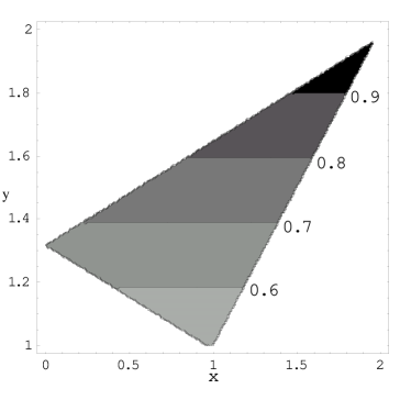
Figure 1: Contour plot of $q{\rm Im}\Pi_{s,s^{\prime}}(q,\omega)$ in units of ($m^{2}/\pi$) for $s^{\prime}=-s=1$ at $B=10^{16}$ G, $T=10^{9}$ K and density $n=0.155\ {\rm fm}^{-3}$ with $x=\beta q$ and $y=\beta\omega$.

As is illustrated in Fig. 1 for small $T$ the region in the $q$,$\omega$-plane where $q{\rm Im}\Pi(\@vec{q},\omega)$ is finite, is essentially bounded by three straight lines (which become exact limits for $T\rightarrow 0$); these boundaries are essentially determined by the fact that $q<\omega$ and the condition $p_{\rm{min}}\leq p^{-}_{Fn}$ . The latter can also be expressed (neglecting all terms in $p_{\rm{min}}$ except the leading order terms in $m$) as $\omega\geq h^{-},\omega\leq h^{+}$ with $h^{\pm}\approx(2m|\mu_{n}|B\pm p^{-}_{Fn}q)/(m^{2}+(p^{-}_{Fn})^{2})^{1/2}$.

3.2 Emissivity

We have only to consider the case $s^{\prime}=-s=1,$ in which case $M_{ss^{\prime}}^{2}=G_{F}^{2}c^{2}_{A}/{2}$. By integrating over the neutrino momenta in Eq. (3) and introducing the dimensionless parameters $y=\beta\omega$ and $x=\beta q$, the emissivity can be expressed as

$$\epsilon_{\nu\overline{\nu}}=\frac{G_{F}^{2}c^{2}_{A}m^{2}}{2(2\pi)^{5}}T^{7}\int_{0}^{\infty}dy\frac{y^{4}}{e^{y}-1}$$

$$\int_{0}^{y}dx\Bigg{(}\ln\frac{e^{-\beta E_{\rm{min}}}+1}{e^{-\beta E_{\rm{min}}-y}+1}-\ln\frac{e^{-\beta E_{\rm{max}}}+1}{e^{-\beta E_{\rm{max}}-y}+1}\Bigg{)}.$$ (9)

To obtain some insight in the dependence of the emissivity on $B$ we distinguish three different regions of $B$ (for simplicity we take $|q|=\omega$, so that the integral over $x$ can be replaced by $2y/5$)

• For weak magnetic fields ($|\mu_{n}|B\ll T$) the region in which $E_{min}<0$ is proportional to $\mu_{n}B/T$ and peaks around $y\approx\mu_{n}B/T$. For $y\ll 1$ one obtains

  $$\epsilon_{\nu\overline{\nu}}\approx\frac{G_{F}^{2}c^{2}_{A}m^{2}}{30(2\pi)^{5}}T^{7}(y_{max}^{6}-y_{min}^{6}),$$ (10)

  where $y_{max/min}=\left(2\mu_{n}B/mT\right)(\sqrt{m^{2}+(p^{-}_{Fn})^{2}}\pm p^{-}_{Fn}).$ Hence for fixed $T$, one finds

  $$\epsilon_{\nu\overline{\nu}}\propto B^{6}.$$ (11)

• For strong magnetic fields ($|\mu_{n}|B\sim T$) the Bose function in Eq. (9) must be kept and the emissivity becomes

  $$\epsilon_{\nu\overline{\nu}}\approx\frac{G_{F}^{2}c^{2}_{A}m^{2}}{5(2\pi)^{5}}T^{7}\int_{y_{min}}^{y_{max}}dy\frac{y^{6}}{e^{y}-1}.$$ (12)

  The integral peaks around $|\mu_{n}|B\approx 3T$ with a width $6T(p^{-}_{Fn}/m)$. As discussed in section 7 for $B$ values in the range $|\mu_{n}|B\sim T$ the emissivity becomes comparable to conventional (modified Urca) process.

• From Eq. (9) we see that for superstrong magnetic fields ($|\mu_{n}|B\gg T$) the emissivity falls off exponentially with the magnetic field for fixed $T$.

4 Neutrino-pair bremsstrahlung from protons  ($p\rightarrow p+\nu+\overline{\nu}$)

In a magnetized matter in addition to the spin-magnetic field interaction the charged particles (protons, electrons) are grouped into Landau levels. The proton’s Fermi momentum in a magnetic field for given Landau level number $N$ and spin $s$ is given by (see Appendix A)

$$p^{s,N}_{Fp}=(E^{2}_{Fp}-m^{2}-(2N+1-sg_{p})eB)^{1/2},$$

where $g_{p}$ is the proton $g$-factor.
The population of Landau levels leads to a smearing of the transverse momentum, $\Delta p_{\perp}\sim\sqrt{eB},$ and as a consequence the condition for energy/momentum conservation is softened. In the special case of a superstrong magnetic field, $eB>(p^{+0}_{Fp})^{2}$, only the lowest ($N=0$) Landau level is occupied.

4.1 Emissivity

In the present case it is convenient to define a reduced proton polarization function for a specific Landau level $N=p^{2}_{\perp}/(2eB)$

$${\rm Im}\Pi_{N^{\prime},N,s^{\prime},s}(q_{z},\omega_{z})=\int dp_{z}[f(E_{pz,N,s})-$$

$$f(E_{pz^{\prime},N^{\prime},s^{\prime}})]\,\delta(E_{pz,N,s}-E_{pz^{\prime},N^{\prime},s^{\prime}}+\omega_{z}+U_{N^{\prime},N}),$$ (13)

where $\omega_{z}=(\omega^{2}-\omega_{\perp}^{2})^{1/2}$ with $\omega_{\perp}=(q^{2}_{x}+q^{2}_{y})^{1/2}$, $U_{N^{\prime},N}$ is the energy difference between the Landau levels $N,N^{\prime}$ and the proton energies $E_{pz,N,s}$ are defined in Appendix A. In evaluating Eq. (13) the integral over $p_{z}$ is replaced by $(m/p^{s,N}_{Fp})\int dE_{pz,N,s},$ and after integration over $E_{pz,N,s}$ one obtains

$${\rm Im}\Pi_{N^{\prime},N,s^{\prime},s}(q_{z},\omega_{z})=\frac{m}{p^{s,N}_{Fp}}[f(\tilde{E}_{a})+f(\tilde{E}_{b})$$

$$-f(\tilde{E}_{a}+\omega_{z}+U_{N^{\prime}N})-f(\tilde{E}_{b}+\omega_{z}+U_{N^{\prime}N})]$$ (14)

with

$$\tilde{E}_{a,b}=(m^{2}+\tilde{p}^{2}_{a,b}+(2N+1-sg_{p})eB)^{1/2},$$ (15)

where $\tilde{p}_{a}$ and $\tilde{p}_{b}$ follow from the condition of conservation of $z$-momentum and energy. To obtain real solutions for $\tilde{p}_{a}$ and $\tilde{p}_{b}$ the conditions $d\equiv(q^{2}_{z}-\omega^{2}_{z}+4m\mu_{p}B)^{2}-4m^{2}(\omega^{2}_{z}-q^{2}_{z})>0$ (neglecting some small terms) and $s=-s^{\prime}=1$ should be satisfied. The result for $\tilde{p}_{a}$ and $\tilde{p}_{b}$ is

$$\tilde{p}_{a,b}(q_{z},\omega_{z})=\frac{|-(4m\mu_{p}B+q^{2}_{z}-\omega^{2}_{z})q_{z}\pm\omega_{z}\sqrt{d}|}{2(\omega^{2}_{z}-q^{2}_{z})}.$$ (16)

We note that the polarization function essentially vanishes unless $\tilde{p}_{a}$ and $\tilde{p}_{b}$ are close to the Fermi momentum $p^{s,N}_{Fp}=\sqrt{(p_{Fp}^{s,0})^{2}-2NeB}$. In the case of a superstrong magnetic field only the $N^{\prime}=N=0$ states are occupied and the contribution to ${\rm Im}\Pi_{N^{\prime},N,s^{\prime},s}(q_{z},\omega_{z})$ comes only from the lines in the $\omega_{z}$,$q_{z}$-plane defined by (neglecting all terms in $p_{{a}}$ except the leading order terms in $m$)

$$\omega_{z}^{\pm}\approx\frac{2m\mu_{p}B\pm q_{z}p_{Fp}^{+0}}{\sqrt{m^{2}+2(1-g_{p})m\mu_{B}B+(p_{Fp}^{+0})^{2}}}.$$ (17)

For weaker $B$-fields a larger space in the $q_{z}$,$\omega_{z}$-plane contributes eventually leading to a situation similar to that for neutrino-pair bremsstrahlung from neutrons.
The emissivity can be written as

$$\epsilon_{\nu\overline{\nu}}=\sum_{N^{\prime},N,s^{\prime},s}\frac{6}{4(2\pi)^{4}}\int d\omega\,dq_{z}\,d\omega_{z}\,g_{B}(\omega)\,\frac{\omega^{4}}{6}$$

$${\rm Im}\Pi_{N^{\prime},N,s^{\prime},s}(q_{z},\omega_{z})\,|M_{N^{\prime},N,s^{\prime},s}|^{2},$$ (18)

where

$$|M_{N^{\prime},N,s^{\prime},s}|^{2}=\sum_{R^{\prime}R}|{\cal M}_{R^{\prime},R,N^{\prime},N,s^{\prime},s}|^{2}=\frac{eB}{2\pi}$$

$$\frac{G_{F}^{2}}{4}[c_{V}^{2}\delta_{s^{\prime},s}+2c_{A}^{2}\delta_{s^{\prime},-s}+c_{A}^{2}\delta_{s^{\prime},s}]I^{2}_{N^{\prime},N}(v)$$

with $v=(\omega^{2}-\omega^{2}_{z})/(2eB)$, $R$ and $R^{\prime}$ the guiding center quantum numbers and $I_{N,N^{\prime}}$ the associated Laguerre polynomials (see Appendix A). As in the case of neutron bremsstrahlung only one spin configuration contributes ($s=-s^{\prime}=1$). For strong magnetic fields, $B\gg T^{2}/(4m\mu_{B})$, the dominant contribution to the emissivity comes from $N^{\prime}=N$ in which case the weak interaction matrix can be simplified in case of $Nv\ll 1$

$$\sum_{R^{\prime},R}|{\cal{M}}^{2}_{R^{\prime},R,N,N,-,+}|^{2}=\frac{G_{F}^{2}}{2}c_{A}^{2}\frac{eB}{2\pi}I^{2}_{N,N}(v)$$

$$\approx\frac{G_{F}^{2}}{2}c_{A}^{2}\frac{eB}{2\pi}.$$ (19)

Using the fact that $U_{N^{\prime}N}$ vanishes for $N^{\prime}=N$, in this case the emissivity becomes

$$\epsilon_{\nu\overline{\nu}}=\sum_{N=0}^{N_{max}}\frac{24mc^{2}_{A}G_{F}^{2}\mu_{B}BT^{7}}{4(2\pi)^{5}}\int dy\frac{1}{e^{y}-1}\frac{y^{4}}{6}$$

$$\int_{0}^{y}dy_{z}\int_{0}^{y_{z}}dx_{z}\,{\rm Im}\Pi_{N,N,-,+}(x_{z},y_{z}),$$ (20)

where $y=\omega/T$, $y_{z}=\omega_{z}/T$, $x_{z}=q_{z}/T$ and $N_{max}=(p^{+0}_{Fp})/(4m\mu_{B}B)$. In weak magnetic fields when eq. (19) is not a good approximation, the summation over $N$ must be restricted to $(4m\mu_{B}B)/(36T^{2})$. In general the integral over $x_{z}$ must be carried out numerically. In case of $\mu_{p}B\approx T$ the main contribution comes from $y_{z}=y$, and as a result the emissivity of neutrino-pair bremsstrahlung from protons is very similar to neutrino-pair bremsstrahlung from neutrons. On the other hand for weaker fields the emissivity of neutrino-pair bremsstrahlung from protons is larger due to the smearing of the transverse momenta of the protons.

5 Direct Urca process  ($n\rightarrow p+e+\overline{\nu}_{e}$; $p+e\rightarrow n+\nu_{e}$)

It is well known that the direct Urca process can occur only if the Fermi momenta satisfy the inequality

$$p_{Fp}+p_{Fe}>p_{Fn}$$ (21)

(except for a small thermal smearing), i.e. the proton concentration $x_{p}={n_{p}}/(n_{p}+n_{n})$ needs to be larger than 1/9 (Lattimer et al. Lat2 (1991)). Recently it was shown (Leinson & Perez Leinson (1998); Baiko & Yakovlev Baiko (1999)) that the presence of a magnetic field has an effect on the Urca process; in particular it leads to a non-vanishing emission rate in case the triangular condition (21) is not satisfied (the so-called classically forbidden region). This is caused by a smearing of the momenta in the presence of a magnetic field which leads to a softening of the sharp border between the allowed and forbidden regimes. Since the emissivities due to the Urca process in superstrong $B$-fields (Leinson & Perez Leinson (1998)) and in arbitrary $B$-fields (Baiko & Yakovlev Baiko (1999)) have been derived previously, we provide below a brief discussion for the purpose of completeness.

5.1 Emissivity

The emissivity is calculated using the quasi-particle approximation for the polarization function where the electrons and protons occupy the Landau levels $N_{e}$, $N_{p}$, respectively,

$$\epsilon_{\nu\overline{\nu}}=2\sum_{N_{e}N_{p}s_{n}s_{p}}\frac{1}{(2\pi)^{6}}\int d^{3}p_{n}\,dp_{ez}d^{3}p_{\nu}\,dp_{pz}$$

$$\delta(p_{nz}-p_{pz}-p_{ez}-p_{{\nu}z})\sum_{R_{e}R_{p}}|{\cal M}_{R_{e},R_{p},N_{e},N_{p},s_{n},s_{p}}|^{2}$$

$$\omega_{\nu}f(E^{n})(1-f(E^{p}))(1-f(E^{e}))$$

$$\delta(E^{n}+V_{np}-E^{p}-E^{e}+\omega_{\nu}),$$ (22)

where $V_{np}=E_{Fp}+E_{Fe}-E_{Fn}$ and the neutron, proton, and electron energies are given in Appendix A and the matrix element ${\cal M}$ in Appendix B. The factor 2 comes from the contribution of the inverse reaction.

5.1.1 Superstrong magnetic fields

First we consider superstrong magnetic fields where the electrons and protons populate the ground state Landau levels ($N_{e}=N_{p}=0$) with spin parallel to $B$, so that $|p_{pz}|\approx p^{+0}_{Fp}$ and $|p_{ez}|\approx p^{0}_{Fe}$. Neglecting the neutrino momentum the matrix element in Eq. (22) simplifies to $\sum_{R_{e}R_{p}}|{\cal M}|^{2}=C_{s_{n}}\exp(-p^{2}_{n\perp}/2eB)$ with $C_{s_{n}}=G_{F}^{2}[(1-2c_{A}+c^{2}_{A})\delta_{s_{n},1}+4c^{2}_{A}\delta_{s_{n},-1}]/2,$ and $p^{2}_{n\perp}=(p^{s_{n}}_{Fn})^{2}-(p_{pz}+p_{ez})^{2}$. Evaluating the energy integrals leads to

$$\epsilon_{\nu\overline{\nu}}=\sum_{s_{n}}C_{s_{n}}\frac{4(120+6\pi^{2})Be}{(2\pi)^{5}}\frac{m_{n}m_{p}}{p^{+0}_{Fp}}T^{6}$$

$$(\Theta(p^{s_{n}}_{Fn})\exp[-(p^{s_{n}}_{Fn})^{2}/2eB]+\Theta(p^{s_{n}}_{Fn}-|p^{+0}_{Fp}+p^{0}_{Fe}|)$$

$$\exp[-((p^{s_{n}}_{Fn})^{2}-(p^{+0}_{Fp}+p^{0}_{Fe})^{2})/2eB]).$$ (23)

The $\Theta$ functions correspond to conservation of momentum in the $z$-direction; it is worth noting that the triangular condition expressing the momentum conservation in the presence of a superstrong $B$-field, $|p^{+0}_{Fp}+p^{0}_{Fe}|<|p^{s_{n}}_{Fn}|$, is the opposite of the one found for the $B$=0 case.
The expression (23) for the emissivity has been obtained previously by Leinson & Perez (Leinson (1998)) and Baiko & Yakovlev (Baiko (1999)) . The factor $C_{+}=G_{F}^{2}(1-c_{A})^{2}/2$ in Eq. (23) agrees with the result of Baiko & Yakovlev (Baiko (1999)), but differs from the one given by Leinson & Perez (Leinson (1998)).

5.1.2 Weak magnetic fields

In the case of weak magnetic fields, i.e. $eB<p^{2}_{Fp}$, the summation over the Landau levels in Eq. (22) is replaced by an integral. Also the $I_{NN}$ functions in the matrix element given by Eq. (74) of Appendix B are replaced by their small-$B$ asymptotes

$$2eB\sum_{N_{e}N_{p}}I^{2}_{N_{e}N_{p}}(v)\rightarrow$$

$$\frac{1}{2Be}\int dp^{2}_{e\perp}dp^{2}_{p\perp}A(p_{p\perp},p_{e\perp},B)\,Ai^{2}(z)$$ (24)

with $Ai(z)$ being the Airy function with

$$z=\frac{[p^{2}_{n\perp}-(p_{p\perp}+p_{e\perp})^{2}](p_{p\perp}+p_{e\perp})^{1/3}}{(2eB)^{2/3}(p_{p\perp}+p_{e\perp})^{4/3}},$$

$v=p^{2}_{n\perp}/2eB$, and

$$A(p_{p\perp},p_{e\perp},B)=\frac{(2eB)^{2/3}}{(p_{p\perp}+p_{e\perp})^{2/3}(p_{p\perp}p_{e\perp})^{1/3}}.$$

Neglecting the neutrino momentum in the $z$-direction in the delta function in Eq. (22) in comparison with the momenta in the $z$-direction of the other particles and performing the integral over $d\cos(\theta_{n})$, the emissivity can be written as (Baiko & Yakovlev Baiko (1999))

$$\epsilon_{\nu\overline{\nu}}=\frac{8(1+3c^{2}_{A})G_{F}^{2}(120+6\pi^{2})m_{n}m_{p}p_{Fp}p^{2}_{Fe}}{(2\pi)^{5}eB}$$

$$\int d\cos(\theta_{p})\,d\cos(\theta_{e})\,A(p_{p\perp},p_{e\perp},B)\,Ai^{2}(z)$$

$$\delta(p_{Fn}-|p_{Fp}\cos(\theta_{p})+p_{Fe}\cos(\theta_{e})|).$$ (25)

In the classically forbidden domain for the direct Urca process for finite $B$ the reaction becomes possible due to the tunnelling mechanism. In the quasi-classical approach the emissivity can be expressed as (Baiko & Yakovlev Baiko (1999))

$$\epsilon_{\nu\overline{\nu}}^{forbidden}(B\neq 0)=R(x,y)\ \epsilon_{\nu\overline{\nu}}^{allowed}(B=0)$$ (26)

with

$$R(x,y)\approx\sqrt{\frac{y}{x+12y}}\,\frac{3}{x^{3/2}}\,\exp(\frac{-x^{3/2}}{3}),$$ (27)

where $y=N_{Fp}^{2/3}=(p_{Fp}^{2}/(2eB))^{2/3}$ and $x$ is a measure of the violation of the triangular condition,

$$x=\frac{p^{2}_{Fp}-(p_{Fp}+p_{Fe})^{2}}{p^{2}_{Fp}N^{-2/3}_{Fp}}.\$$ (28)

One sees that with increasing $x$, the emissivity decreases exponentially, and therefore the effect is important only if $p_{Fn}$ does not exceed $(p_{Fp}+p_{Fe})$ significantly.
On the other hand in the classically allowed region, where the inequality is satisfied, the $B$-field will give rise to small quantum oscillations of the emissivity.

6 Equation of state (EoS)

In order to estimate the effect of a magnetic field on the various cooling processes in a neutron star and to compare with the conventional result we employ a simple model EoS. It is assumed that the neutron star matter consists of neutrons, protons and electrons only ($npe$-matter) with two conditions imposed: charge neutrality, $n_{p}=n_{e}$, and $\beta$-equilibrium, $\phi_{n}=\phi_{p}+\phi_{e}$. The EoS consists of the energy density as a function of the densities of the particles. The non-relativistic energy density can be decomposed as (Lattimer & Swesty Lattimer (1991); Balberg & Gal Balberg (1997))

$$E=E_{kin}+E_{mag}+E_{mass}+E_{pot}+E_{lep}.$$ (29)

Here the kinetic energy density is the sum of the neutron

$$E^{n}_{kin}=\frac{3}{5}\sum_{s_{n}}\frac{(p^{s_{n}}_{Fn})^{2}}{2m_{n}}n^{s_{n}}_{n}$$ (30)

and proton contribution

$$E^{p}_{kin}=\frac{1}{3}\sum_{s_{p}}\frac{(p^{s_{p},0}_{Fp})^{2}}{2m_{p}}n^{s_{p}}_{p},$$ (31)

where the proton density for spin $s_{p}$ is

$$n^{s_{p}}_{p}=\sum_{N}\frac{eB}{2\pi^{2}}\sqrt{(p^{s_{p},0}_{Fp})^{2}-2NeB},$$ (32)

because for finite $B$ the integrals over the transverse momentum of the proton with respect to the magnetic field can be replaced by a summation over the Landau levels. The interaction of the magnetic field with the spin of the neutron and the proton is

$$E_{mag}=-\mu_{n}B\sum_{s_{n}}s_{n}n^{s_{n}}_{n}-\mu_{p}B\sum_{s_{p}}s_{p}n^{s_{p}}_{p}.$$ (33)

The $E_{mass}$ term contains the masses of the two nucleons

$$E_{mass}=m_{n}\sum_{s_{n}}n^{s_{n}}_{n}+m_{p}\sum_{s_{p}}n^{s_{p}}_{p}.$$ (34)

The $E_{pot}$ term is the potential energy density, which is parametrized as (Lattimer & Swesty Lattimer (1991))

$$E_{pot}=an^{2}+bn^{1+d}+\sum_{s_{n},s_{p}}4cn^{s_{n}}_{n}n^{s_{p}}_{p},$$ (35)

where $n=n_{p}+n_{n}$ is the total nucleon density. The last term on the rhs of Eq. (35), which corresponds to the symmetry energy, influences to a large extent the proton fraction $n_{p}/(n_{p}+n_{n})$. Finally the energy density of the electrons is

$$E_{lep}=E_{Fe}n_{e},$$ (36)

where

$$n_{e}=\sum_{N_{e}}\frac{g_{N_{e}}eB}{2\pi^{2}}\sqrt{(p_{Fe}^{0})^{2}-2N_{e}eB}$$ (37)

with $g_{N_{e}}=1$ for $N_{e}=0$, $g_{N_{e}}=2$ for $N_{e}>0$ and $N_{e}$ is limited from above by $N_{e}^{max}=(p^{0}_{Fe})^{2}/(2eB)$.
We obtain the EoS of the $npe$-matter in magnetic fields in the standard manner, by assuming a given nucleon density $n$ and $T=0$ and solving the equations of charge neutrality and $\beta$-equilibrium. In two limiting cases the solutions are straightforward.
i) $B=0$. The summations over the proton and electron concentration in Eqs. (32) and (37) can be replaced by integrations and the densities $n_{e}$, $n_{p}$ and $n_{n}$ can be calculated in the standard way using $n_{i}=p^{3}_{Fi}/(3\pi^{2})$. Using the $\beta$-equilibrium condition, $\phi_{e}=\phi_{n}-\phi_{p}$, the chemical potential of the electron is given by

$$\phi_{e}=\frac{(3\pi^{2}n_{n})^{2/3}}{2m_{n}}-\frac{(3\pi^{2}n_{p})^{2/3}}{2m_{p}}+4c(n_{p}-n_{n})+\Delta$$ (38)

with $\Delta$ the mass difference between neutron and proton.
ii) Superstrong magnetic fields, $(p^{+0}_{Fp})^{2}<(2eB)$, in which case the protons and electrons are in the ground state Landau level. Then the electron chemical potential is

$$\phi_{e}=\frac{1}{2}\sum_{s_{n}}\frac{(6\pi^{2}n^{s_{n}}_{n})^{2/3}}{2m_{n}}-\frac{1}{2m_{p}}\Big{(}\frac{2\pi^{2}n_{p}}{eB}\Big{)}^{2}$$

$$+\frac{g_{p}-1}{2m_{p}}\,eB+4c(n_{p}-n_{n})+\Delta.$$ (39)

In this case the proton fraction depends on the magnetic field. In Eq. (35) we take $d=2$, $a=-285.1\ {\rm MeV}\ {\rm fm}^{3}$, $b=968\ {\rm MeV}\ {\rm fm}^{6}$, $c=-107.1\ {\rm MeV}\ {\rm fm}^{3}$ (Lattimer & Swesty Lattimer (1991)).

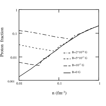
Figure 2: Proton fraction as a function of density for various B-fields

In Fig. 2 the resulting proton fraction in the absence and in the presence of magnetic fields is plotted. The kinks in the proton fraction at certain densities correspond to the occupation of a next Landau level (see also Suh & Mathews Suh (1999)). For superstrong magnetic fields these kinks strongly influence the proton fraction, but for weaker magnetic fields ($B\leq 10^{17}G$ and $n\geq n_{0}$ where $n_{0}=0.155\ {\rm fm}^{-3}$ is the saturation density) they do not affect the proton fraction. Our results are in agreement with the previous results for the proton fraction derived from different equations of state (Lai & Shapiro Lai (1991); Suh & Mathews Suh (1999), Broderick, Prakash and Lattimer Bro (2000)).

7 Results

The emissivities for the various energy loss processes are compared in Figs. 3, 4 and 5 for $n=n_{0}$ for three different magnetic field strengths ($10^{16}$,$10^{17}$ and $2\times 10^{18}$ G, respectively).

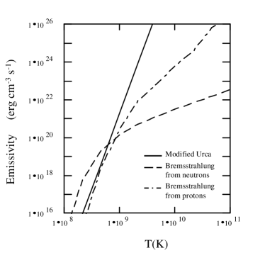
Figure 3: Emissivities of various processes at saturation density $n=n_{0}$ and for $B=10^{16}{\rm G}$. The contribution of the direct Urca process is negligible.

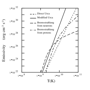
Figure 4: Same as in Fig. 3 but for $B=10^{17}{\rm G}$.

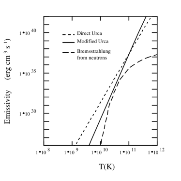
Figure 5: Same as in Fig. 2 but $B=2\times 10^{18}{\rm G}$

In the first two values of the $B$-field the EoS based on $B=0$ is used (because in these cases the influence of the magnetic field on the EoS itself is small); for the third value of the $B$-field we use the EoS for superstrong magnetic fields.
To enable a comparison with the neutrino processes which are routinely included in the cooling simulations of neutron stars, we show also the emissivity due to the modified Urca process in the zero field limit. The relevant expression for the emissivity of the modified Urca process, without corrections for the magnetic field, and valid for $m^{*}=m$ is (Friman & Maxwell FM (1979))

$$\epsilon_{\nu\overline{\nu}}=1.8\times 10^{21}(n/n_{0})^{2/3}T_{9}^{8}\ {\rm ergs}\ {\rm cm}^{-3}\ {\rm s}^{-1}$$ (40)

with $T_{9}$ the temperature in units of $10^{9}$ K.

The temperature region where the one-body neutrino-pair bremsstrahlung is important increases with increasing magnetic field (Figs. 3 and 4). The pair bremsstrahlung from neutrons is efficient whenever $|\mu_{n}|B\sim T$, since then the energy involved in the spin-flip is of the same order of magnitude as the thermal smearing of the Fermi surface. The temperature at which neutrino-pair bremsstrahlung from neutrons becomes comparable to the competing processes roughly coincides with this condition. For lower temperatures the emissivity drops exponentially, because the energy transfer becomes larger than the thermal smearing. Neutrino-pair bremsstrahlung from protons is important when $\mu_{p}B\sim T$. The emissivity due to the protons increases faster than the emissivity due to the neutrons with the temperature, as the smearing of the proton transverse momenta provides an additional relaxation on the kinematical constrains. However for temperatures smaller than $\mu_{p}B\sim T$ the emissivity drops just as for neutrons exponentially.
As seen from Figs. 3 and 4 the emissivity of the modified Urca process is larger than that of neutrino-pair bremsstrahlung from neutrons and protons at high temperatures mainly due to the different temperature dependencies of these processes ($\propto T^{7}$ for the one-body bremsstrahlung as compared to $\propto T^{8}$ for the modified Urca). In the case of a superstrong magnetic field the large uncertainty in the transverse momenta of the protons and electrons allows the direct Urca process to occur (see Fig. 5) and its emissivity dominates the emissivity of any other processes.

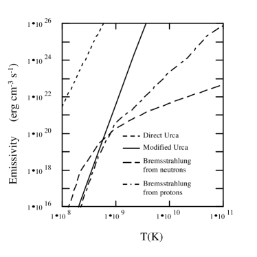
Figure 6: Emissivity at $n=3n_{0}$ and $B=10^{16}{\rm G}$.

In Fig. 6 the emissivities are shown for $n=3n_{0}$ and $B=10^{16}$ G. At this density the triangle condition $p_{Fp}+p_{Fe}>p_{Fn}$ is satisfied, so that the direct Urca process is allowed and dominates the cooling. The emissivities of the other processes are slightly larger than those shown in Fig. 3 due to the fact that the density is larger.

8 Conclusion

We have studied the neutrino emissivity of strongly magnetized neutron stars due to the one-body processes driven by the charged and neutral current couplings between the neutrinos and baryons. We have shown that, in addition to the well-known charged current process (the direct Urca reaction), there is a new channel of energy loss - the one-body neutrino pair-bremsstrahlung in a magnetic field. The process does not have an analogue in the zero field limit and competes with the modified (two-body) bremsstrahlung process as the dominant neutral current reaction for fields on the order $10^{16}-10^{17}$ G and temperatures a few times $10^{9}$ K. For superstrong magnetic fields in excess of $10^{18}$ G the direct Urca process takes over.
Our numerical evaluation of the emissivities of several competing reactions, which is based on a simple parametrization of the EOS of $npe$-matter in a strong magnetic field, shows that under certain conditions the emissivities of the one-nucleon processes, such as the direct Urca and the one-body bremsstrahlung, are of the same order of magnitude or dominate the standard processes commonly included in the cooling simulations in the zero-field limit.

Appendix A Electrons, protons and neutrons in a magnetic field

The wave equation for a fermion with charge $q$ and mass $m$ can be written as (Itzykson & Zuber Itzykson (1980)):

$$(i\not\partial+q\not A-(m-\frac{\Delta g}{2}\mu_{B}\sigma^{\mu\nu}F_{\mu\nu})),\Psi(x)=0,$$ (41)

with $\mu_{B}=e/2m$, $\not\partial=\gamma_{\mu}\partial^{\mu}$, $\not A=\gamma_{\mu}A^{\mu}$ and $\Delta g$ the anomalous gyromagnetic factor. Here $\gamma^{\mu}$ is a Dirac matrix, $A^{\mu}$ the vector potential, $F_{\mu\nu}=\partial_{\mu}A_{\nu}-\partial_{\nu}A_{\mu}$ and $\sigma^{\mu\nu}=\frac{i}{2}[\gamma^{\mu},\gamma^{\nu}]$. Or equivalently

$$((i\partial+qA)^{2}+\frac{q}{2}\sigma^{\mu\nu}F_{\mu\nu}-$$

$$(m-\frac{\Delta g}{2}\mu_{B}\sigma^{\mu\nu}F_{\mu\nu})^{2})\Psi(x)=0.$$ (42)

In particular, if one chooses the Landau gauge $A^{\mu}=(0,-\frac{By}{2},\frac{Bx}{2},0)$ with the magnetic field in the $z$-direction, one finds

$$((i\partial+qA)^{2}+sqB-(m-\Delta gs\mu_{B}B)^{2})\Psi(x)=0.$$ (43)

A.1 Electron

For an electron ($q=-e$ and $\Delta g=0$) the energy eigenvalues are given by

$$E_{N,s}=(m^{2}+p^{2}_{z}+2NeB)^{1/2},$$ (44)

with $N$ denoting the Landau level number. The eigenfunctions are factorized (Sokolov & Ternov ST (1968); Arras & Lai Arras (1999))

$$\psi_{e}=e^{ip_{z}z-iE_{N,s}t}U_{e}(\rho,\phi),$$

$$U_{e}(\rho,\phi)=\sqrt{\frac{eB}{2\pi}}e^{i(N-R)\phi}\left(\begin{array}[]{l}V_{a}I_{N-1,R}(t)e^{-i\phi}\\ iV_{b}I_{N,R}(t)\\ V_{c}I_{N-1,R}(t)e^{-i\phi}\\ iV_{d}I_{N,R}(t)\\ \end{array}\right)$$ (49)

and

$$I_{N,R}(t)=\sqrt{\frac{R!}{N!}}e^{-t/2}t^{(N-R)/2}\tilde{L}_{R}^{N-R}(t),$$

where $\tilde{L}_{R}^{M}(t)$

$$=\left\{\begin{array}[]{llr}L_{R}^{M}(t)&\ {\rm if}&\ \ M\geq 0\\ (-1)^{|M|}t^{|M|}L^{|M|}_{R-|M|}(t)&\ {\rm if}&\ \ M<0\end{array}\right.$$

with $t={\rho}^{2}eB/2$, $V_{a}=C_{+}D_{+}$, $V_{b}=\sigma C_{-}D_{+}$, $V_{c}=\sigma C_{+}D_{-}$, $V_{d}=C_{-}D_{-}$,

$$C_{\pm}=\frac{1}{\sqrt{2}}\left(1\pm\sigma\frac{p_{z}}{(p^{2}_{z}+4m\mu_{B}BN)^{1/2}}\right)^{1/2},$$

$$D_{\pm}=\frac{1}{\sqrt{2}}\left(1\pm\frac{m}{E}\right)^{1/2},$$

and $\sigma$ is the longitudinal spin projection along $\@vec{p}+e\@vec{A}$; $L_{R}^{M}(t)$ is the generalized Laguerre function. The Landau level number $N$ and the guiding center quantum number $R$ are positive integers. (Note that in the lowest energy state ($N=0)$ the spin $s$ can only have the value -1).
In matter in the presence of a magnetic field the Fermi energy is given by $E_{F}=(m^{2}+(p^{N}_{Fe})^{2}+2NeB)^{1/2}$ so that a magnetic field will give rise to a difference in the Fermi momenta $p^{N}_{Fe}$. The degeneracy is 1 in case of $N=0$ and 2 in case of $N>0$.

A.2 Proton

For a proton ($q=e$ and $\Delta g=g_{p}-1$ with $g_{p}=2.79$) the energy eigenvalues (neglecting the $B^{2}$-term) are

$$E_{N,s}=(m^{2}+p^{2}_{z}+(2N+1-sg_{p})eB)^{1/2}.$$ (50)

The non-relativistic eigenfunction of a proton in a magnetic field is

$$\psi_{p}=e^{ip_{z}z-iE_{N,s}t}U_{p}(\rho,\phi),$$

$$U_{p}(\rho,\phi)=\sqrt{\frac{eB}{2\pi}}e^{i(R-N)\phi}\left(\begin{array}[]{l}\delta_{s,1}I_{R,N}(t)\\ \delta_{s,-1}I_{R,N}(t)\\ 0\\ 0\\ \end{array}\right).$$ (51)

(Note that the role of $R$ and $N$ are interchanged compared to the electron case.) In matter the Fermi energy is given by $E_{F}=(m^{2}+(p^{s,N}_{Fp})^{2}+(2N+1-sg_{p})eB)^{1/2}$.

A.3 Neutron

For a neutron ($q=0$ and $\Delta g=g_{n}$ with $g_{n}=-1.91$) in not extremely large magnetic fields the $B^{2}$-term can be neglected; then the energy eigenvalues are

$$E_{s}=(m^{2}+p^{2}-2sg_{n}m\mu_{B}B)^{1/2},$$ (52)

and the eigenfunction are simple plane waves. In neutron matter in thermal equilibrium the Fermi energy is given by $E_{F}=(m^{2}+(p^{s}_{Fn})^{2}-2sg_{n}m\mu_{B}B)^{1/2}$. Hence the neutrons with spin up (down) occupy two Fermi spheres with Fermi momenta related by $(p^{+}_{Fn})^{2}=(p^{-}_{Fn})^{2}+4m\mu_{n}B$.

Appendix B The weak interaction matrix elements

B.1 Neutrino-neutron interaction (neutral current)

The weak interaction matrix for the neutron bremsstrahlung is

$$M_{s,s^{\prime}}=\frac{G_{F}}{2\sqrt{2}}\int_{V}d\mathbf{r}\overline{\psi}_{n1}\gamma_{\mu}(c_{V}-c_{A}\gamma_{5})\psi_{n2}\overline{\psi}_{\nu}\gamma^{\mu}(1-\gamma_{5})\psi_{\overline{\nu}}.$$ (53)

Here $c_{V}$ and $c_{A}$ are vector and axial-vector coupling constants. The interaction matrix consists of a hadronic part and a leptonic part

$$|M_{s,s^{\prime}}|^{2}=\frac{G_{F}^{2}}{8}X_{\mu\nu}L^{\mu\nu}$$ (54)

with the leptonic part given by

$$L^{\mu\nu}=\frac{2}{pp^{\prime}}[p^{\mu}p^{\prime\nu}-g^{\mu\nu}(p\cdot p^{\prime})+p^{\nu}p^{\prime\mu}+i\epsilon^{\alpha\mu\beta\nu}p_{\alpha}p^{\prime}_{\beta}],$$

and the hadronic part by

$$X_{\mu\nu}=\left(\begin{array}[]{cccc}c^{2}_{V}\delta_{s,s^{\prime}}&0&0&-s^{\prime}c_{V}c_{A}\delta_{s,s^{\prime}}\\ 0&c^{2}_{A}\delta_{s,-s^{\prime}}&ic^{2}_{A}s\delta_{s,-s^{\prime}}&0\\ 0&-ic^{2}_{A}s\delta_{s,-s^{\prime}}&c^{2}_{A}\delta_{s,-s^{\prime}}&0\\ -s^{\prime}c_{V}c_{A}\delta_{s,s^{\prime}}&0&0&c^{2}_{A}\delta_{s,s^{\prime}}\end{array}\right).$$ (59)

Contracting the hadronic and leptonic tensors and neglecting terms, which after integration over the neutrino momenta vanish one finds

$$|M_{s,s^{\prime}}|^{2}=\frac{G_{F}^{2}}{4}[(c^{2}_{V}+c^{2}_{A})\delta_{s,s^{\prime}}+2c^{2}_{A}\delta_{s,-s^{\prime}}]$$ (60)

with $c_{V}=1$ and $c_{A}=1.26$.

B.2 Neutrino-proton interaction (neutral current)

In case of protons the integration over space coordinates requires special attention, because the wave functions of protons are not simple plane waves (Eq. 51). Defining $\@vec{\omega}_{\perp}={(p_{{\nu}x}+p_{\overline{\nu}x})}\hat{e}_{x}+{(p_{{\nu}y}+p_{\overline{\nu}y})}\hat{e}_{y}$, $\@vec{x}_{\perp}=x\hat{e}_{x}+y\hat{e}_{y}$, $v=\omega^{2}_{\perp}/2eB$ and carrying out the summations over $R^{\prime}$ and $R$, leads to

$$\sum_{R^{\prime},R}|{\cal M}_{R^{\prime},R,N^{\prime},N,s^{\prime},s}|^{2}=\sum_{R^{\prime},R}\frac{eB}{2\pi}|M_{s^{\prime},s}|^{2}$$

$$\bigg{|}\int_{0}^{\infty}\rho d\rho I_{R^{\prime},N^{\prime}}(t)I_{R,N}(t)$$

$$\int_{0}^{2\pi}d\phi e^{-i(R^{\prime}-N^{\prime})\phi}e^{i(R-N)\phi}e^{-i\@vec{\omega}_{\perp}\@vec{x}_{\perp}}\bigg{|}^{2}$$

$$=|M_{s^{\prime},s}|^{2}\frac{eB}{2\pi}I^{2}_{N^{\prime},N}(v)$$ (61)

with $c_{V}=-0.08$ and $c_{A}=-1.26$.

B.3 Direct Urca process (charged current)

The interaction matrix is

$${\cal M}_{R_{e},R_{p},N_{e},N_{p},s_{n},s_{p}}=\frac{G_{F}}{\sqrt{2}}\int_{V}d\mathbf{r}\overline{\psi}_{p}\gamma_{\mu}(c_{V}-c_{A}\gamma_{5})\psi_{n}$$

$$\overline{\psi}_{e}\gamma^{\mu}(1-\gamma_{5})\psi_{\overline{\nu}}.$$ (62)

The eigenfunctions of the electron, proton and neutron are given in Appendix A. The function $I_{R_{p},N_{p}}(t)$ with $t=\rho^{2}eB/2$ can be substituted in the leptonic part. The hadronic part turns out the same as for the neutron bremsstrahlung (see Eq. 54). The space integrals can be calculated in the same way as in Eq. (61) with the result

$$L_{\mu\nu}=\frac{1}{2p}\sum_{s_{e}=\pm 1}{\rm Tr}[Y_{e}\gamma_{\mu}(1-\gamma_{5})\not p\gamma_{\nu}(1-\gamma_{5})\overline{Y_{e}}]$$

with

$$Y_{e}=\left(\begin{array}[]{l}V_{a}I_{N_{e}-1,N_{p}}(v)\\ iV_{b}I_{N_{e},N_{p}}(v)\\ V_{c}I_{N_{e}-1,N_{p}}(v)\\ iV_{d}I_{N_{e},N_{p}}(v)\\ \end{array}\right),$$ (68)

where $v=q^{2}/2eB$ with $q={(p_{{\nu}x}+p_{nx})}\hat{e}_{x}+{(p_{{\nu}y}+p_{ny})}\hat{e}_{y}$. The expression for $D$ appearing in the expressions for in $V_{i}$ ($i=a,b,c$ and $d$) can be approximated by $D\approx 1/\sqrt{2}$. This leads to the following expression for the leptonic part

$$\mathbf{L^{\mu\nu}}=\left(\begin{array}[]{cccc}J_{+}(v)&0&0&J_{-}(v)\\ 0&J_{+}(v)&iJ_{-}(v)&0\\ 0&-iJ_{-}(v)&J_{+}(v)&0\\ J_{-}(v)&0&0&J_{+}(v)\end{array}\right)$$ (73)

with $J_{\pm}(v)=I^{2}_{N_{e},N_{p}}(v)\pm I^{2}_{N_{e}-1,N_{p}}(v)$. As a result the following relation is obtained for the squared norm of the interaction matrix

$$\sum_{R_{e}R_{p}}|{\cal M}_{R_{p},R_{e},N_{p},N_{e},s_{n},s_{p}}|^{2}=\frac{G^{2}}{2}\frac{eB}{2\pi}(\delta_{s_{p},s_{n}}(c^{2}_{V}+c^{2}_{A})$$

$$(I^{2}_{N_{e},N_{p}}(v)+I^{2}_{N_{e}-1,N_{p}}(v))$$

$$+2\delta_{s_{p},s_{n}}g_{a}s_{p}(I^{2}_{N_{e}-1,N_{p}}(v)-I^{2}_{N_{e},N_{p}}(v))$$

$$+2\delta_{s_{p},-s_{n}}g^{2}_{a}(\delta_{s_{p},1}\ I^{2}_{N_{e},N_{p}}(v)+$$

$$\delta_{s_{p},-1}\ I^{2}_{N_{e}-1,N_{p}}(v)))$$ (74)

with $c_{V}=1$ and $c_{A}=1.26$.

- (1) Arras P., Lai D., 1999, Phys. Rev. D60, 043001
- (2) Baiko D.A., Yakovlev D.G., 1999, AA 342, 192
- (3) Balberg S., Gal A., 1997, Nucl. Phys. A625, 435
- (4) Bandyopadhyay D., Chakrabarty S., Dey P., Pal S., 1998, Phys. Rev. D58, 121301
- (5) Bocquet M., Bonazzola S., Gourgoulhon E., Novak J., 1995, AA 301, 757
- (6) Broderick A., Prakash M., Lattimer J.M., 2000, astro-ph/0001537
- (7) Cline T., Frederiks D.D., Golenetskii S., et al., 1999, astro-ph/9909054, to appear in ApJ
- (8) Duncan R.C., Thompson C., 1992, ApJ 392, L9
- (9) Friman B.L., Maxwell O.V., 1979, ApJ 232, 541
- (10) Gotthelf E.V., Vasisht G., Dotani T., 1999, ApJ 522, L49
- (11) Haberl F., Hotch C., Buckley D.A.H., Ziekgraf F.-J., Pietsch W., A&A 326, 662
- (12) Haensel P., Urpin V.A., Yakovlev D.G., 1990, AA 229, 133
- (13) Horowitz C.J., Gang Li, 1998, Phys. Rev. Lett. 80, 3694
- (14) Itzykson C., Zuber J.-B., 1980, Quantum field theory, McCraw Hill, New York, p. 64
- (15) Kouveliotou C., Dieters S., Strohmayer T., et al., 1998, Nat 393, 235
- (16) Lai D., Shapiro S.L., 1991, ApJ 383, 745
- (17) Lattimer J.M., Swesty F.D., 1991, Nucl. Phys. A535, 331
- (18) Lattimer J.M., Pethick C.J., Prakash M., Haensel P., 1991, Phys. Rev. Lett. 66, 2701
- (19) Leinson L.B., Perez A., 1998, JHEP 9, 20
- (20) Mattuck R.D., 1992, A guide to Feynman diagrams in the many-body problem (dover, New York)
- (21) Mazets E.P.,Golenetskii S.V., Il’inskii V.N., et al., 1979, Nat 282, 587
- (22) Murakami T., Tanaka Y., Kulkarni S.R., et al., 1994, Nat 368, 127
- (23) van Paradijs J., Taam R.E., van den Heuvel E.P.J., 1995, A&A 299, L41
- (24) Raffelt G., Seckel D., 1995, Phys. Rev. D52, 1780
- (25) Rho J., Petre R., 1997, ApJ 484, 828
- (26) Sedrakian A., Dieperink A., 1999, Phys. Lett. B 463, 145; astro-ph/0002228
- (27) Shapiro S.L., Teukolsky S.A., 1983, Black Holes, White Dwarfs and Neutron Stars, John Wiley and Sons, New York, p. 316
- (28) Sokolov A.A., Ternov I.M., 1968, Synchrotron Radiation, Akademie-Verlag, Berlin
- (29) Suh I.-S., Mathews G.J., 1999, astro-ph/9912301
- (30) Thompson C., Duncan R.C., 1995, MNRAS 275, 255
- (31) Vasisht G., Gotthelf E.V., 1997, ApJL 486, L129
- (32) Voskresensky D.N., Senatorov A.V., 1986, Sov. Phys. JETP 63, 885
- (33) Woods P., Kouveliotou C., van Paradijs J., Hurley K., Kippen R.U., 1999, ApJ 519, L139