Pairing Gaps from Nuclear Mean–Field Models

Abstract

We discuss the pairing gap, a measure for nuclear pairing correlations, in chains of spherical, semi–magic nuclei in the framework of self–consistent nuclear mean–field models. The equations for the conventional BCS model and the approximate projection–before–variation Lipkin–Nogami method are formulated in terms of local density functionals for the effective interaction. We calculate the Lipkin–Nogami corrections of both the mean–field energy and the pairing energy. Various definitions of the pairing gap are discussed as three–point, four–point and five–point mass–difference formulae, averaged matrix elements of the pairing potential, and single–quasiparticle energies. Experimental values for the pairing gap are compared with calculations employing both a delta pairing force and a density–dependent delta interaction in the BCS and Lipkin–Nogami model. Odd–mass nuclei are calculated in the spherical blocking approximation which neglects part of the the core polarization in the odd nucleus. We find that the five–point mass difference formula gives a very robust description of the odd–even staggering, other approximations for the gap may differ from that up to $30\%$ for certain nuclei.

1 Introduction

Pair correlations, which play a crucial role in superconducting solids Bar57a , also constitute an important complement of nuclear shell structure Boh58a ; Bel58a . Most often, pairing is treated in the so–called BCS approximation EGIII ; Ringbook ; Nilssonbook , which was introduced in the original paper of Bardeen, Cooper and Schrieffer Bar57a . The nuclear applications are particular in two respects: first, nuclei are finite, in fact rather small, objects, and second, we do not yet have a sufficiently reliable microscopic nuclear many–body theory from which we could deduce the appropriate pairing interaction and its strength. The second problem causes two further questions. First, one needs to develop a reliable and manageable form for the pairing energy functional, and second, one has to determine an appropriate pairing strength for a given functional.

There exist various prescriptions for the pairing energy functional. Schematic pairing forces basically consist of defining a small band of pairing–active states and parameterizing one typical pairing matrix element in dependence on the system size, i.e. neutron and proton number. They are convenient and successful in many respects. But they are plagued by serious disadvantages: the coupling to continuum states is much exaggerated and the parameterization in terms of system size becomes questionable for deformed systems along the fission path. To avoid these problems local two–body pairing forces are increasingly used which is particularly satisfying in connection with self–consistent mean–field calculations Ton79a ; Kri90a ; Dob95a ; Dob96c . There are even some mean–field models like the Gogny forces Dob96c ; Gogrev or the particular Skyrme force SkP Dob84a which aim at a simultaneous description of the particle–particle and particle–hole channels of the effective interaction using the same force. That is not a necessary condition. The simple local pairing energy functionals also provide a very good description of pairing properties throughout the whole chart of isotopes using only two universal strength parameters, one for protons and one for neutrons. This makes these forms for the pairing energy functional more reliable for calculations of deformed nuclei and of nuclei far off the valley of stability than the widely used schematic pairing forces. In the following we will concentrate on the class of local pairing interactions.

The small particle number of nuclei often interferes with the fact that the BCS ground state mixes particle numbers with a relative spread of order $1/\sqrt{N}$. In principle, one has to perform a projection of the BCS state before variation, but this exact particle number projection can be very cumbersome, see, e.g., Mang ; MONSTER . The Lipkin–Nogami (LN) scheme offers a reliable approximate projection method Lip60a ; Nog64a ; Pra73a ; Flo . It has the technical advantage that it is formulated completely in terms of BCS expectation values which makes its numerical implementation very simple, for detailed discussion see Pra73a ; Flo ; Zhe92a ; Dob92a . We will discuss the LN scheme side by side with the BCS treatment.

There remains as the last and crucial problem the determination of an appropriate pairing strength. Insufficient microscopic information requires that one recurs to a phenomenological assessment. This line of development has been followed with increasing accuracy since the introduction of pairing in nuclei, for a comprehensive compilation of pairing with schematic forces see Mol92a . Also the local two–body pairing interactions leave the overall strength as a free parameter to be fixed phenomenologically. This has to be done with respect to an observable sensitive to pairing correlations. Such an observable would ideally be provided by the pairing gap which, however, is not directly accessible in experiments. The observable quantity with probably closest relation to the pairing gap is the pronounced odd–even mass staggering of nuclei, which is usually used for fitting the pairing strength. Even here, though, there remains a choice of several recipes on how to extract the pairing gap or odd–even staggering, respectively, from a combination of neighboring mass values. From the theoretical side, of course, one has more direct access to a gap. But even there ambiguities emerge and one is left with several possibilities to define measures for the pairing correlations.

It is the aim of this paper to compare and discuss the various definitions of a pairing gap in models of local two-body pairing interactions in connection with self–consistent mean–field approaches, both at the level of the conventional BCS approach as well as of the LN method. Furthermore, we will compare two variants of the local zero–range pairing forces, a delta force and a density–dependent form Dob95a ; Dob96c . Last but not least, the discussion will extend to exotic nuclei where differences between the various definitions for the pairing gap and options for the pairing method become particularly obvious.

The paper is outlined as follows: In Section 2 we present the basic equations of the Lipkin–Nogami model employing local interactions in the framework of the Skyrme–Hartree–Fock model needed for our discussion. In Section 3 various approximations for the pairing gap are discussed, in Section 4 the results are presented, Section 5 summarizes our findings.

2 The Theoretical Framework

We investigate the pairing gap in the framework of self–consistent mean–field models. Pairing correlations are treated on the HF+BCS level where the equations of motion are derived by independent variation with respect to single–particle wave functions and occupation amplitudes. This is a widely used approximation to the more involved HFB approach where wave functions and occupation amplitudes are varied simultaneously Ringbook . The BCS approximation is applicable for all well–bound nuclei, i.e. for most of the nuclei discussed throughout this paper. It becomes critical only for nuclei close to the neutron or proton drip–line, see e.g. Dob84a , and such nuclei are not considered here. All conclusions about pairing gaps drawn in this paper can thus safely be derived in the BCS approximation.

2.1 The Mean Field

Presently the most widely used self–consistent mean–field models are the non–relativistic Hartree–Fock approach with either the Skyrme (SHF) SHFrev or the Gogny force Gogrev , and the relativistic mean–field model RMFrev . They all provide a well-adjusted effective energy functional for nuclear mean–field calculations. We choose the SHF model for the present investigation. The description starts from an energy functional

$${\cal E}={\cal E}_{\rm mf}+{\cal E}_{\rm pair}\quad,$$ (1)

whose mean–field part ${\cal E}_{\rm mf}$ is formulated in terms of the local distributions of density $\rho$, kinetic density $\tau$, and spin–orbit current ${\bf J}$. At this point it is not necessary to unfold all details of this rather elaborate functional, we abbreviate the dependence with the most general case, the full one–body density matrix

$$\hat{\rho}\equiv\rho(\vec{x},\vec{x}^{\prime})=\langle\hat{\psi}^{\dagger}(\vec{x}^{\prime})\hat{\psi}(\vec{x})\rangle$$ (2)

from which all local densities and currents can be derived, see appendix A.2 for details. $\hat{\psi}^{\dagger}(\vec{x})$ creates a particle with spin projection $\sigma/2$ at the space point $\vec{r}$. Throughout this paper $\langle\cdots\rangle$ denotes BCS expectation values. For the Skyrme energy functional we choose the rather recent parameterization SkI4 Rei95a . The pairing energy functional depends additionally on the local pair density $\chi$ as introduced in Section 2.2. Variation of the energy functional ${\cal E}$ with respect to the single–particle wave functions $\phi_{k}$ yields the mean–field equations

$$\hat{h}\,\phi_{k}=\varepsilon_{k}\,\phi_{k}\quad\mbox{with}\quad\hat{h}=\frac{\delta{\cal E}}{\delta\hat{\rho}}\quad,$$ (3)

where we have neglected the contributions from the variation of the pairing density $\chi$ in the energy functional to the equations–of–motion of the single–particle states $\phi_{k}$. This constitutes the BCS approximation to pairing (see Rei97a for the discussion of the full HFB equations in the representation in natural orbitals that is used here). The mean–field equations are solved on a grid in coordinate space with the damped gradient iteration method and a Fourier representation of the derivatives. The numerical techniques are summarized in Blum .

2.2 The Pairing Energy Functional

We parameterize the effective pairing interaction in terms of a local pairing energy functional of the form

$${\cal E}_{\rm pair}=\frac{1}{4}\sum_{q\in\{p,n\}}\int\!{\rm d}^{3}r\;\chi_{q}^{*}(\textbf{r})\;\chi_{q}(\textbf{r})\;G_{q}(\textbf{r})\quad,$$ (4)

which allows for a spatial modulation of the strength $G(\textbf{r})$. $\chi(\textbf{r})$ is the local part of the pair density matrix

$$\chi_{q}(\vec{r}) = \sum_{\sigma=\pm}\chi_{q}(\vec{r},\sigma;\vec{r},\sigma)=-\sum_{\sigma=\pm}\sigma\;\langle\hat{\psi}_{q}(\vec{r},-\sigma)\hat{\psi}_{q}(\vec{r},\sigma)\rangle$$ (5)

$$= -2\sum_{k\in\Omega_{q}\atop k>0}u_{k}\,v_{k}\,|\phi_{k}(\textbf{r})|^{2}\quad,$$

with $q\in\{p,n\}$. The $\phi_{k}$ are the single–particle wave functions and $v_{k}$, $u_{k}=\sqrt{1-v_{k}^{2}}$ the pairing amplitudes. We restrict ourselves to stationary states of time–reversal invariant systems and pairing between like particles only. This sorts the single–particle states into conjugate pairs $k\leftrightarrow\bar{k}\equiv-k$ with the same spatial properties but opposite projection of the total angular momentum and allows to restrict the summation in the pair density to $k>0$. The time–reversal symmetry also renders the pair density real, i.e. $\chi^{*}({\mbox{\bf r}})=\chi({\mbox{\bf r}})$.

Two models for the spatial modulation of the pairing strength are considered here

$$G_{q}({\textbf{r}})=\left\{\begin{array}[]{lll}V_{0,q}&&\mbox{DF,}\\ V_{0,q}\;\bigg{[}1-\left({\displaystyle\frac{\rho({\mbox{\bf r}})}{\rho_{0}}}\right)^{\gamma}\bigg{]}&&\mbox{DDDI.}\end{array}\right.$$ (6)

The simpler case (DF) can be deduced from a delta force for the pairing interaction Ton79a ; Kri90a ; Dob95a , $V_{\rm pair}(\textbf{r},\textbf{r}^{\prime})=V_{0,q}\;\delta(\textbf{r}-\textbf{r}^{\prime})$, while the other (DDDI) corresponds to a density–dependent delta interaction Dob95a ; Taj93b ; Fay94a . The additional parameters of the DDDI force are set here to $\gamma=1$ and $\rho_{0}=0.16\;{\rm fm}^{-3}$ (i.e. the saturation density of symmetric nuclear matter). More general choices are conceivable Dob84a ; Fay96a but very hard to adjust phenomenologically. Thus we keep to the simplest choice above. Note that a separate pairing strength $V_{0,p}$ or $V_{0,n}$ is associated to each nucleon sort. This explicit breaking of the isospin symmetry in the pairing energy functional is standard in nearly all pairing forces and schematic models, see e.g. Mol92a ; Mad88a .

Although the pairing matrix elements deduced from the pairing functional (4) suppress the contribution from unbound states located outside the nucleus considerably (as compared to the schematic pairing force), the implicit zero–range nature of the pairing force still tends to overestimate the coupling to continuum states. This defect can be cured to some extent using finite–range forces like the Gogny force Dob96c ; Gogrev which are, however, cumbersome to handle. We prefer to simulate the effect of finite range by introducing smooth energy–dependent cutoff weights Kri90a

$$f_{k}=\frac{1}{1+\exp[(\epsilon_{k}-\lambda_{q}-\Delta E_{q})/\mu_{q}]}$$ (7)

in the evaluation of the local pair density

$$\chi_{q}(\textbf{r})\Rightarrow-2\sum_{k\in\Omega_{q}\atop k>0}f_{k}\,u_{k}\,v_{k}\,|\phi_{k}(\textbf{r})|^{2}\quad.$$ (8)

The cutoff parameters $\Delta E_{q}$ and $\mu_{q}=\Delta E_{q}/10$ are chosen self–adjusting to the actual level density in the vicinity of the Fermi energy. $\Delta E_{q}$ is fixed from the condition that the sum of the cutoff weights includes approximately one additional shell of single-particle states above the Fermi surface

$$\sum_{k\in\Omega_{q}}f_{k}=N_{q}+1.65\,N_{q}^{2/3}\quad.$$ (9)

2.3 The Lipkin–Nogami Equations

The LN scheme serves as an approximation to particle–number projected BCS. It can be derived by a momentum expansion of the projected BCS equations Lip60a ; Nog64a ; Pra73a ; Flo . At the end this boils down to adding overlaps with the variance of the particle number $(\Delta\hat{N}_{q})^{2}$ at various places.

In most cases, the LN method is used with a simple schematic pairing interaction in the framework of macroscopic–microscopic models and self–consistent models for ground states and potential energy surfaces Mol92a ; Ben89a ; Naz90a ; Que90a ; Taj92a ; Hee93a ; Ska93 ; Mag95a ; Rei96a as well as high–spin states Mag93a ; Sat94a ; Sat94b ; Gal94a ; Wys95a ; Hee95a ; Ter95 . Only recently, the LN scheme was employed for a local delta pairing force Cwi96a and the Gogny force Val96a ; Val97a . Usually only the correction of the pairing energy is calculated; but in self–consistent models the contribution of the mean field to the total binding energy is calculated from the BCS state as well, so that the correction of the pairing energy has to be complemented by a correction of the mean–field energy as considered in Rei96a ; Val96a ; Val97a . In this paper, we present and employ the LN equations in the context of self–consistent mean–field models and for the case of local pairing energy functionals. As pairing gaps are the theme of this paper, particular emphasis is laid on the properties of the LN scheme relevant for the discussion of pairing gaps.

The LN equations are derived by variation of

$${\cal K}={\cal E}-\sum_{q\in p,n}\Big{(}\lambda_{1,q}\langle\hat{N}_{q}\rangle+\lambda_{2,q}\langle\hat{N}_{q}^{2}\rangle\Big{)}\quad.$$ (10)

Variation of (10) with respect to the occupation amplitudes $v_{k}$ leads to

$$v_{k}^{2}=\frac{1}{2}\left[1-\frac{\epsilon_{k}^{\prime}-\lambda_{q}}{\sqrt{(\epsilon_{k}^{\prime}-\lambda_{q})^{2}+f_{k}^{2}\;\Delta_{k}^{2}}}\right]\quad.$$ (11)

This is the standard expression for the occupation number $v_{k}^{2}$ in the BCS model EGIII ; Ringbook ; Nilssonbook , here containing a state–dependent single–particle gap $\Delta_{k}$ times the cutoff factor $f_{k}$ and a generalized Fermi energy

$$\lambda_{q}=\lambda_{1,q}+4\lambda_{2,q}(N_{q}+1)\quad,$$ (12)

which is determined from a constraint on particle number. The quantity $\epsilon_{k}^{\prime}$ is a renormalized single–particle energy

$$\epsilon_{k}^{\prime}=\epsilon_{k}+4\,\lambda_{2,q}v_{k}^{2}\quad.$$ (13)

In case of time-reversal invariance, the state–dependent single–particle gaps are given by

$$\Delta_{k}=\int\!{\rm d}^{3}r\;\phi_{k}^{\dagger}(\textbf{r})\Delta_{q}(\textbf{r})\phi_{k}(\textbf{r})\quad,$$ (14)

i.e. they are matrix elements of the local pair potential

$$\Delta_{q}(\textbf{r})=\frac{\delta{\cal E}_{\rm pair}}{\delta\chi_{q}(\textbf{r})}=\frac{1}{2}\;\chi_{q}(\textbf{r})\;G_{q}(\textbf{r})\quad.$$ (15)

Note that $\lambda_{2}$ is not a Lagrange parameter Flo ; Que90a . It is held fixed during the variation and is determined after variation from the additional condition Pra73a

$$\lambda_{2,q}=\frac{\langle(\hat{H}_{\rm mf}+\hat{H}_{\rm pair})(\Delta\hat{N}_{2,q})^{2}\rangle}{\langle\hat{N}_{q}(\Delta\hat{N}_{2,q})^{2}\rangle}\quad.$$ (16)

For simplicity of the presentation, Eq. (16) is written for the case of an underlying many–body Hamiltonian $\hat{H}$. The discussion of the more general case of an energy functional used in this paper is presented in Appendix A.1. $\hat{N}_{2,q}$ is the part of the particle–number operator that projects onto two–quasiparticle states

$$\hat{N}_{2,q}=\sum_{k\in\Omega_{q}}u_{k}v_{k}\,(\hat{\alpha}^{\dagger}_{k}\hat{\alpha}^{\dagger}_{\bar{k}}+\hat{\alpha}_{\bar{k}}\hat{\alpha}_{k})\quad,$$ (17)

while $\Delta\hat{N}_{2,q}=\hat{N}_{2,q}-\langle\hat{N}_{2,q}\rangle$. The numerator of Eq. (16) contains, besides the familiar contribution from the pairing functional, an additional one from the linear response of the mean–field to the particle–number projection, see Rei96a . The total binding energy after approximate particle–number projection is given by

$$E^{\rm LN}={\cal E}-\sum_{q\in{\rm p,n}}\lambda_{2,q}\;\langle(\Delta\hat{N}_{2,q})^{2}\rangle\quad.$$ (18)

For arbitrary one–body operators the LN expectation value can be calculated introducing effective LN occupation numbers and local densities, see Que90a ; Rei96a .

Thus far the presentation applies to the more involved LN method. The BCS approximation is recovered simply by setting $\lambda_{2,q}=0$ in the above equations.

2.4 Blocking

The evaluation of the odd–even staggering involves also nuclei with odd mass number where one pair of conjugate states has to be blocked, i.e. taken out of the pairing scheme. One of the blocked states has the occupation $v_{k}=1$, the other $v_{\bar{k}}=0$. In the standard textbook approach the blocked many–body state is constructed non–self–consistently from the BCS ground state as a one–quasiparticle excitation, see e.g. EGIII ; Ringbook ; Nilssonbook and Section 3.3. The generalization of this approach for energy functionals is outlined in Appendix B.

In a self–consistent approach to the blocked many–body state the single–particle wave functions and occupation amplitudes have to be determined from a variational principle. Blocking a pair of states changes the density matrix, Eq. (2) and with that the single–particle Hamiltonian, Eq. (3). Besides a rearrangement of the single–particle wave functions the unpaired nucleon causes a polarization of the core by breaking rotational and time–reversal invariance in the intrinsic frame (we assume spherical BCS ground states only), see e.g. ugpap . This requires a deformed calculation of the odd–mass nucleus considering also time–odd contributions to the single–particle Hamiltonian (3) as discussed in ugpap ; Dob95c .

The change in binding energy due to the core polarization depends on the properties of the time–odd spin and spin–isospin channels of the effective interaction which are not yet well adjusted for current mean–field models, see e.g. Eng99a and references therein. Calculations with the currently available models suggest that the polarization is non–negligible for the description of the odd–even staggering ugpap ; Sat98a ; Sat98b ; Xu99a ; uggap , but effective interactions with properly adjusted spin and spin–isospin channels are needed before the effect can be treated quantitatively. In view of these uncertainties we restrict ourselves here to the simpler spherical blocking approximation, where one replaces the blocked single–particle state by an average over the degenerate states in its $j$ shell, restoring rotational and time–reversal invariance of the many–body system in the intrinsic frame. In practice this means that the weight of the blocked $j$ shell is given by $(2j-1)uv$ when calculating the pair density and $(2j-1)v^{2}+1$ when calculating the local densities and currents. All other states enter with their full degeneracy $2j+1$. This approximation includes the large part of the rearrangement effects from monopole polarization, but omits the polarization effects from multipole deformations and time–odd currents.

Owing to the rearrangement effects blocking of the single–particle state with smallest quasiparticle energy (as defined in Sect. 3.3) does not necessarily lead to the largest possible total binding energy. Therefore one has to perform calculations for a number of blocked single–particle states around the Fermi energy and search for the configuration giving the largest total binding energy.

3 The Pairing Gap

3.1 Nuclear Masses and Odd–Even Staggering

The key feature of pairing correlations is the occurrence of an energy gap in the excitation spectrum. This gap manifests itself in two different kinds of energetic observables: First, there is a gap in the quasiparticle excitation spectra of even–even nuclei, which does not appear in the spectra of odd–mass number or odd–odd nuclei, and second, there occurs a shift between the interpolating curves of the ground–state binding energies of even–even as compared to odd–mass nuclei, which is called the odd–even mass staggering. Usually, the second phenomenon is exploited to define the experimental pairing gaps assuming Mad88a

$$E_{\rm even-even}(Z,N) = E_{0}(Z,N)\quad,$$

$$E_{{\rm odd}\;Z}(Z,N) = E_{0}(Z,N)+\Delta_{\rm p}(Z,N)\quad,$$ (19)

$$E_{{\rm odd}\;N}(Z,N) = E_{0}(Z,N)+\Delta_{\rm n}(Z,N)\quad.$$

In odd–odd nuclei there is additionally the residual interaction between the unpaired proton and neutron, but this case will not be considered in the present discussion. In a self–consistent mean–field approach $E_{0}$ is the (negative) energy of the fully paired many–particle wave function, i.e. the BCS ground state, while $\Delta_{q}$ is the energy lost due to the blocking of a pair of conjugate states by the odd nucleon. The gap introduced with (3.1) has to be interpreted carefully. The gap as defined through the separation (3.1) contains more than pure pairing correlations. It includes unavoidably all polarization effects from the mean field as outlined in Sect. 2.4. Despite of these uncertainties (3.1) provides the starting point for the definition of experimentally accessible pairing gaps which will be discussed in Sect. 3.2. The gap defined with (3.1) serves than as a point of reference, as it can be calculated directly within the mean–field model

$$\Delta^{({\rm b})}(Z,N):=E_{\rm block}(Z,N)-E_{0}(Z,N)$$ (20)

as the difference in binding energy between the one blocked state of an odd–mass number nucleus with the largest binding energy and its fully paired (fictitious) BCS vacuum. Both calculations have, of course, to be performed self–consistently. We will call $\Delta^{({\rm b})}$ the “blocking gap” in the following.

3.2 Finite–Difference Formulae

The gap from Eq. (20) is a purely theoretical construct. The problem is that $E_{0}$ is not measurable for odd–mass nuclei. We need a definition which is also experimentally accessible. It should fulfill two requirements which are useful for the phenomenological adjustment of the pairing strength: first, it should be easy to calculate both theoretically and from experimental data, and second, it should be influenced as little as possible by the properties of the underlying mean field in order to decouple mean–field and pairing properties. The odd–even staggering is related to differences of nuclear masses and as such easy to measure as well as to compute, As outlined above, the odd–even staggering of experimental masses is not a pure measure of pairing correlations, but also has non–negligible contributions from the response of the underlying mean field to the blocking of a single–particle state. Here we can take advantage of the fact that various difference formulae are conceivable and take the recipe which best decouples mean–field and pairing properties.

The odd–even staggering needs to be deduced from energy systematics. To that end, there are several finite–difference formulae in the literature to calculate $\Delta_{q}$ from binding energies of adjacent nuclei. All available finite–difference formulae for $\Delta_{q}$ are derived from the Taylor expansion of the nuclear mass in nucleon–number differences Mad88a ; Jen84a

$$E(N) = \sum_{n=0}^{\infty}\frac{1}{n!}\frac{\partial^{n}E_{0}}{\partial N^{n}}\bigg{|}_{N_{0}}\;(N-N_{0})^{n}+D(N_{0})$$ (21)

where $E_{0}$ is defined in (3.1) and the Gap $D$ given by

$$D=\left\{\begin{array}[]{cl}0&\mbox{even proton and neutron number},\\ \Delta_{\rm n}&\mbox{odd neutron number},\\ \Delta_{\rm p}&\mbox{odd proton number}.\\ \end{array}\right.$$ (22)

The number of the other kind of nucleons is assumed to be even and the same for all terms. Combining the expansion (21) of several adjacent nuclei leads to energy–difference formulae which can be used to approximate the gap $\Delta^{({\rm b})}$. The two–point (first–order) formula leads to the one–nucleon separation energy, which mixes mean–field, single–particle and pairing effects strongly and should better not be used to fit the pairing strength. The next higher–order is the three–point difference

$$E(N_{0}+1)-2E(N_{0})+E(N_{0}-1)$$

$$= \frac{\partial^{2}E_{0}}{\partial N^{2}}\bigg{|}_{N_{0}}+\frac{1}{12}\;\frac{\partial^{4}E_{0}}{\partial N^{4}}\bigg{|}_{N_{0}}$$

$$\quad+\cdots+D(N_{0}+1)-2D(N_{0})+D(N_{0}-1)\quad,$$

Assuming that the gap $D$ varies only slowly with nucleon number and that the remaining contribution from the second derivative of $E_{0}$ is negligible (which is not so well fulfilled in some cases, see Sect. 4.2 and Sat98a ; Sat98b ) this equation can be resolved into an approximative expression for the pairing gap

$$\Delta^{(3)}_{q}(N_{0}) := \frac{\pi_{N_{0}}^{\mbox{}}}{2}\Big{[}E(N_{0}-1)-2E(N_{0})+E(N_{0}+1)\Big{]}$$ (24)

where $\pi_{N_{0}}=(-1)^{N_{0}}$ is the number parity. $\Delta^{(3)}$ calculated from pure HF states without pairing but considering polarization of the mean field is discussed in Refs. Sat98a ; Sat98b in great detail.

The next order corresponds to a four–point difference formula, but this order, employing an even number of nuclei, gives an expression which is asymmetric around the nucleus with $N_{0}$ and therefore offers two choices. With the same assumptions used going from (3.2) to (24), one possibility for the four–point gap is

$$\Delta^{(4)}_{q}(N_{0}) := \frac{\pi_{N_{0}}}{4}\Big{[}E(N_{0}-2)-3E(N_{0}-1)$$ (25)

$$\quad+3E(N_{0})-E(N_{0}+1)\Big{]}\quad.$$

This is an approximation for the gap at $N_{0}-1/2$. The other possible four–point formula gives the gap at $N_{0}+1/2$. The lowest–order derivative of $E_{0}$ hidden in the four–point formula is now of third order.

Although this four–point definition is widely used in the literature Kri90a ; Cwi96a ; BM we prefer the five–point formula

$$\Delta^{(5)}_{q}(N_{0}) := -\frac{\pi_{N_{0}}}{8}\Big{[}E(N_{0}+2)-4E(N_{0}+1)+6E(N_{0})$$ (26)

$$\quad-4E(N_{0}-1)+E(N_{0}-2)\Big{]}\quad,$$

which is symmetric and yields the best decoupling from mean–field effects as we will see. The smooth contributions from the mean field to the gap are further suppressed compared to the lower–order formulae, the remaining derivative of $E_{0}$ entering $\Delta^{(5)}$ is of fourth order.

3.3 Quasiparticle Energies

Another widely used approximation for the pairing gap is to calculate the energy difference (20) by constructing the blocked many–body wave function of an odd–mass number nucleus non–self–consistently from its BCS ground state as a so–called single–quasiparticle excitation EGIII ; Ringbook ; Nilssonbook . The lowest single–quasiparticle energy

$$E_{\rm quasi}=\mbox{min}(E_{k})$$ (27)

– which we will simply denote as “quasiparticle energy” $E_{\rm quasi}$ in the following – is then another approximation for the odd–even staggering. In the LN scheme the $E_{k}$ are given in first–order approximation by

$$E_{k}\approx\sqrt{(\epsilon_{k}^{\prime}-\lambda_{q})^{2}+f_{k}^{2}\Delta_{k}^{2}}+\lambda_{2,q}\quad,$$ (28)

see Appendix B for details. The important difference between $E_{\rm quasi}$ and $\Delta^{({\rm b})}$ is that for $E_{\rm quasi}$ the blocked many–body wave function is not calculated self–consistently.

3.4 Spectral Gaps

The calculation of $\Delta^{(5)}$ from mean–field models is a bit cumbersome since it requires information on five nuclei including nuclei with odd mass number. Moreover, the definition becomes inapplicable to describe the variation of pairing correlations with deformation for a given nucleus. At this point, we could recur to the purely theoretical definition (20) involving a blocked and an unblocked BCS calculation. This still requires involved calculations and can become unwieldy in deformed calculations.

Therefore, a commonly used approach is to estimate the pairing gap from spectral properties of a nucleus. In schematic pairing models using the same pairing matrix element for all states the single–particle gaps (14) turn out to be state–independent and are thus immediately a measure for the pairing correlations. With local forces as used here we obtain state–dependent single–particle gaps $\Delta_{k}$ and have to define an average gap as representative for the strength of the pairing correlations. The authors of Dob84a have proposed to use the average of the single–particle gaps (14) weighted with the occupation probability $v^{2}_{k}$

$$\langle v^{2}\Delta\rangle_{q}=\frac{\sum_{k\in\Omega_{q}}f_{k}\,v_{k}^{2}\,\Delta_{k}}{\sum_{k\in\Omega_{q}}f_{k}\,v_{k}^{2}}\quad.$$ (29)

This definition, however, puts too much weight on deeply–bound states whereas pairing is a mechanism most active near the Fermi surface. We therefore propose an average with the same factor $v_{k}u_{k}$ as it appears in the accumulation of the pair density $\chi(\textbf{r})$, see Eq. (5), yielding the spectral gap as

$$\langle uv\Delta\rangle_{q}=\frac{\sum_{k\in\Omega_{q}}f_{k}\,v_{k}u_{k}\,\Delta_{k}}{\sum_{k\in\Omega_{q}}f_{k}\,u_{k}v_{k}}\quad.$$ (30)

Note that the spectral gaps are an estimate for the pairing gap and therefore the contribution of pairing correlations to the odd–even staggering (20). Assuming that the spectral gaps (29) and (30) are an approximation for the square–root term in (28), approximately particle–number projected spectral gaps are given by

$$\langle v^{2}\Delta\rangle_{q}^{\rm(LN)}=\langle v^{2}\Delta\rangle_{q}+\lambda_{2,q}\quad,$$ (31)

$$\langle uv\Delta\rangle_{q}^{\rm(LN)}=\langle uv\Delta\rangle_{q}+\lambda_{2,q}\quad,$$ (32)

which was proposed by the authors of Cwi96a for the average gap $\langle v^{2}\Delta\rangle^{\rm(LN)}$. These spectral gaps will be discussed and compared with other alternatives for the calculated pairing gap in Section 4.

4 Results and Discussion

4.1 Fit of Pairing Strength

Table 1: Pairing strengths $V_{\rm n}$ for the neutrons and $V_{\rm p}$ for the protons in ${\rm MeV}\;{\rm fm}^{3}$ for the DF and DDDI pairing functionals used in the BCS and LN schemes in connection with SkI4.

DF DDDI Scheme $V_{\rm n}$ $V_{\rm p}$ $V_{\rm n}$ $V_{\rm p}$ BCS $-323$ $-310$ $-999$ $-1146$ LN $-318$ $-250$ $-947$ $-947$

The first step is to determine appropriate pairing strengths $V_{0,q}$ for the DF and the DDDI functionals. We do that on the grounds of the five–point gap $\Delta^{(5)}$ and adjust the pairing strength by fitting calculated values for $\Delta^{(5)}$ to experimental ones for a large set of semi–magic nuclei, i.e. the isotope chains ${}^{44}_{22}\mbox{Ca}$, ${}^{106}_{\;\>56}\mbox{Sn}$–${}^{128}_{\;\>78}\mbox{Sn}$, and ${}^{201}_{119}\mbox{Pb}$–${}^{206}_{124}\mbox{Pb}$, for the neutrons and the isotone chains ${}^{52}_{28}\mbox{Cr}$, ${}^{82}_{50}\mbox{Ge}_{32}$–${}^{94}_{50}\mbox{Ru}_{44}$, ${}^{136}_{\;\>82}\mbox{Xe}_{54}$–${}^{147}_{\;\>82}\mbox{Tb}_{65}$, and ${}^{210}_{126}\mbox{Po}_{84}$–${}^{215}_{126}\mbox{Ac}_{89}$ for the protons. A seperate fit has been performed for each one of the pairing functionals, DF or DDDI, and for each appraoch, BCS or LN. Each nucleon sort, proton or neutron, aquires its own pairing strength adjusted to isotonic chains, or isotopic chains respectively.

The experimental data are taken from Wapstra . The resulting values for the pairing strength are listed in Table 1. We obtain a reasonable fit of the pairing gaps for all pairing schemes, see also Figures 4 (compare “Expt. with $\Delta^{(5)}$) and 8 in what follows. We have checked that the pairing strengths are not significantly changed (i.e. on the order of $1\%$) when fitting instead theoretical $\Delta^{(3)}$ to experimental $\Delta^{(3)}$ or similarly the $\Delta^{(4)}$.

4.2 Comparison of the Finite–Difference Formulae

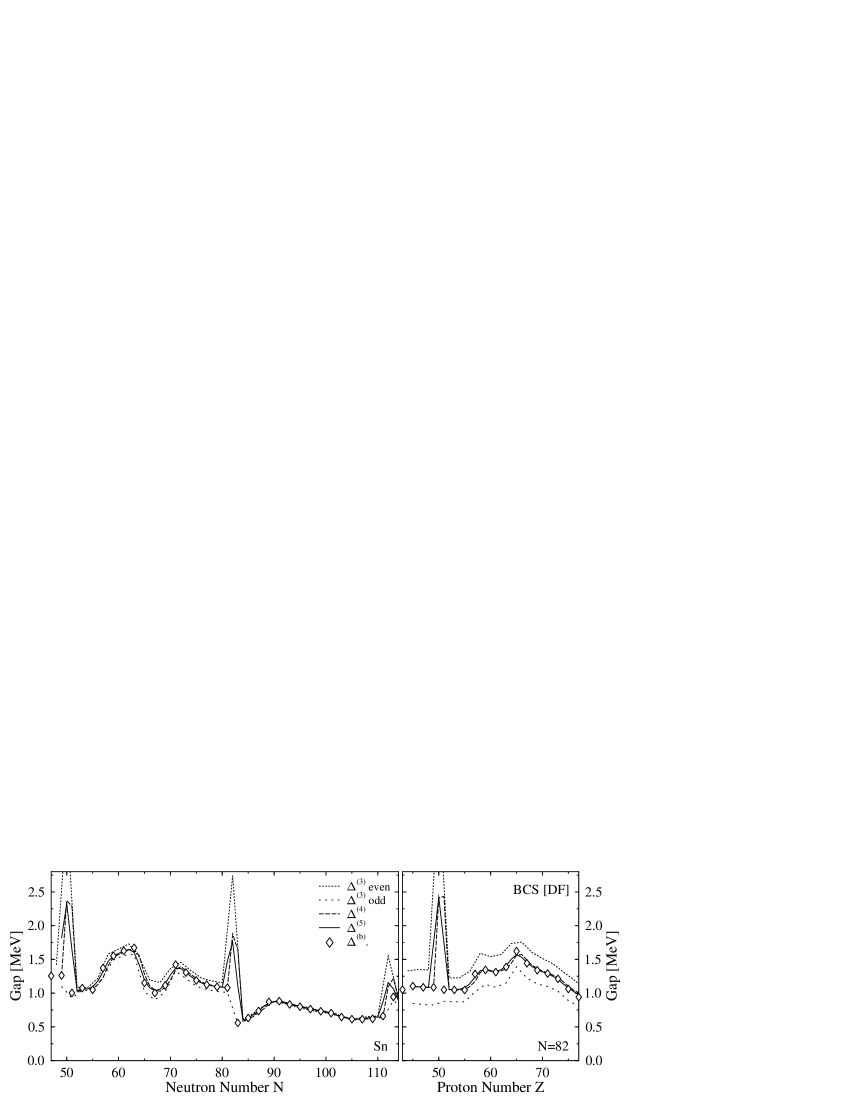
Figure 1: Comparison of the three–point $\Delta^{(3)}$, four–point $\Delta^{(4)}$ and five–point difference formulae $\Delta^{(5)}$ and the blocking gap $\Delta^{({\rm b})}$. The left panel shows results for neutron gaps in the chain of tin isotopes, the right panel for proton gaps in the chain of the $N=82$ isotones.

The various finite–difference gaps were introduced as experimentally accessible approximations to $\Delta^{({\rm b})}$, i.e. the energy differences of blocked and unblocked calculations of odd–mass nuclei. Figure 1 compares directly the performance of the $\Delta^{(i)}$, $i=3,4,5$, in this respect for calculations within the BCS approach. The three–point gaps $\Delta^{(3)}$ show a pronounced odd–even staggering for all $N=82$ isotones and the tin isotopes with neutron numbers below the $N=82$ shell closure. Note that we have disentangled that by drawing a separate line for even–even and odd–mass nuclei. These two lines for $\Delta^{(3)}$ embrace the gap $\Delta^{({\rm b})}$. The staggering is caused by non–vanishing mean–field contributions to $\Delta^{(3)}$ (mainly the second derivative term in Eq. (3.2)), which enter with a different sign for even–even and odd–mass nuclei. The four–point gaps $\Delta^{(4)}$ from Eq. (25) give a smoother approximation for $\Delta^{({\rm b})}$. But as expected the $\Delta^{(4)}$ are slightly shifted versus the $\Delta^{({\rm b})}$ which becomes rather obvious where the gaps change rapidly, e.g. around $N=63$, $N=70$, $Z=57$, $Z=65$. The five–point gaps $\Delta^{(5)}$ give the best overall agreement with the $\Delta^{({\rm b})}$.

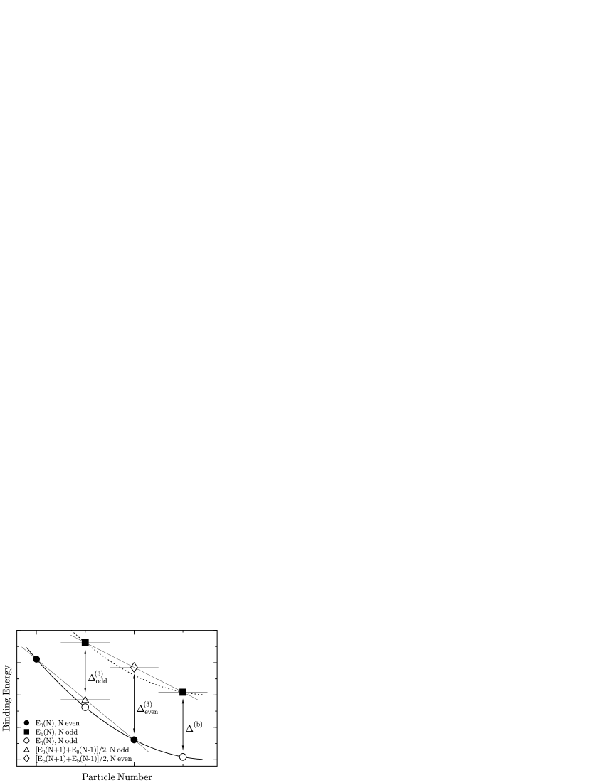
Figure 2: Schematic comparison of $\Delta^{(3)}$ and $\Delta^{({\rm b})}$. $E_{0}$ and $E_{\rm b}$ denote BCS ground–state energies and the energy of the blocked ground state of an odd–mass nucleus respectively. Filled symbols denote binding energies that are experimentally accessible, while the BCS ground state of an odd–mass nucleus (white circles) can be calculated from the mean–field model only.

The oscillation of the $\Delta^{(3)}$ around the values for $\Delta^{({\rm b})}$ has a simple geometrical reason, as can be seen from Fig. 2. $\Delta^{({\rm b})}$ is per definition (20) the shift between the smooth curve connecting the (unblocked) BCS ground–state energies $E_{0}$ of all nuclei (thick line through circles) and the smooth curve that connects the (blocked) ground–state energies $E_{\rm b}$ of odd–mass nuclei (dotted line through full boxes). The three–point gap of an even–even nucleus $\Delta^{(3)}_{\rm even}(N_{0})=\tfrac{1}{2}[E_{\rm b}(N_{0}-1)+E_{\rm b}(N_{0}+1)]-E_{0}(N_{0})$ is the shift between the smooth curve connecting the $E_{0}$ and the average energy of the two adjacent odd–mass nuclei, which lies outside the band given by $\Delta^{({\rm b})}$. From this follows immediately $\Delta^{(3)}_{\rm even}>\Delta^{({\rm b})}$ for bound nuclei. A similar construction leads to $\Delta^{(3)}_{\rm odd}<\Delta^{({\rm b})}$, see Fig. 2. For $\Delta^{(4)}$ and $\Delta^{(5)}$ the deviation from $\Delta^{({\rm b})}$ becomes of course much smaller because the higher–order finite–difference formulae give a better approximation of the smooth curves connecting the $E_{0}$ and $E_{\rm b}$ respectively. This qualitative result does not depend on the level of sophistication for the calculation of the odd–mass–number nuclei. Considering polarization effects will shift $E_{\rm b}$ with respect to $E_{0}$ (which has to be counterweighted by a refit of the pairing strength Xu99a ; uggap ) and may distort the surface of the $E_{\rm b}$, but will not change the sign of its curvature.

There remains a significant difference between all $\Delta^{(i)}$, $i=3,4,5$ and $\Delta^{({\rm b})}$ around shell closures where finite–difference formulae (except $\Delta^{(3)}$ for odd nuclei) produce a peak which becomes broader with increasing order of the difference formula. We want to discuss the origin of this peak for the example of the five–point gap $\Delta^{(5)}$. The five–point approximation (26) for $\Delta^{({\rm b})}$ makes three assumptions: (i) the binding energy is an analytical function of the nucleon numbers and therefore can be expanded in a Taylor series in the range of two mass units around the considered nucleus; (ii) derivatives of $E_{0}$ of higher than third order are negligible; and (iii) the gap varies only slowly with nucleon number. The first two assumptions are strongly violated at shell closures, where the kink in the systematics of binding energies does not allow the Taylor expansion (21) and leads to a spurious contribution from the mean–field functional to the finite–difference gaps.

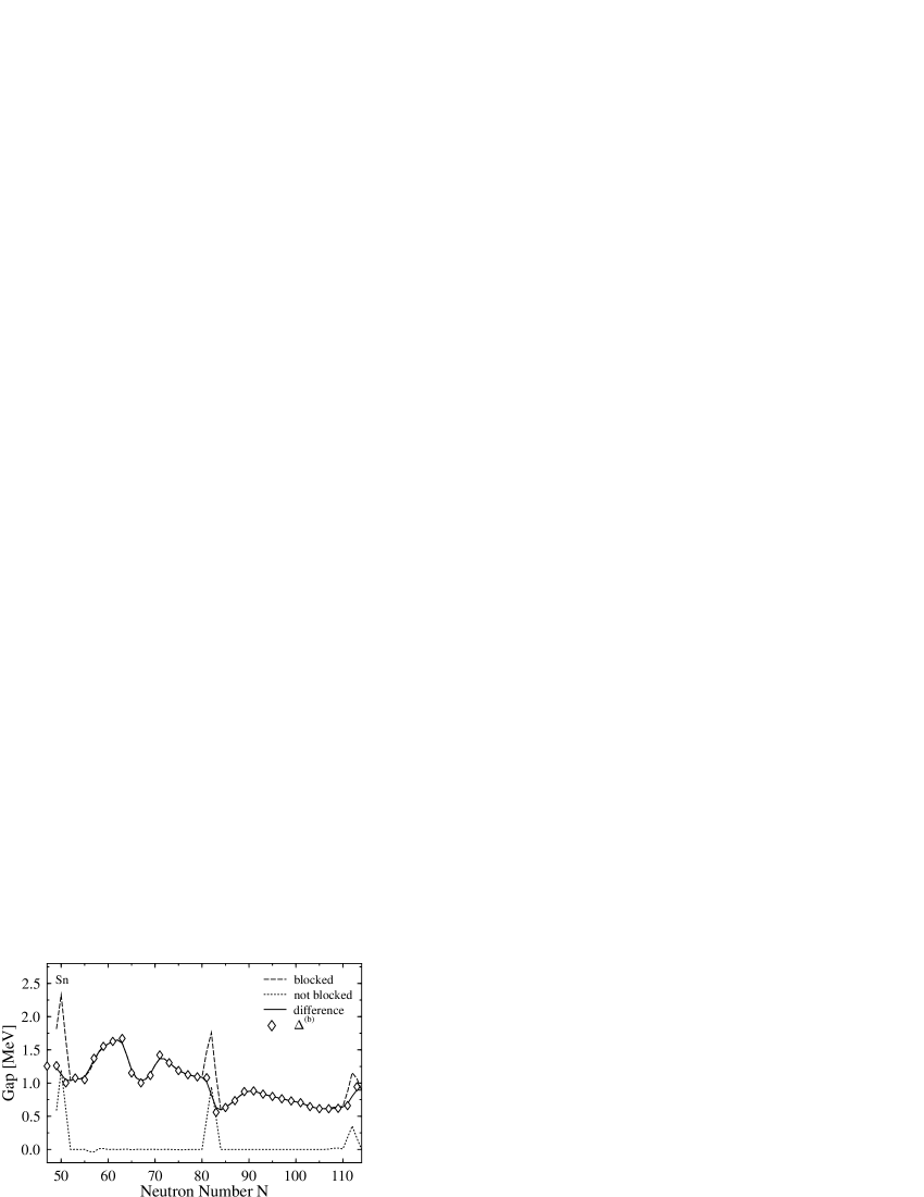
Figure 3: Five–point gaps $\Delta^{(5)}$ computed using either blocked calculations of the odd–mass nuclei (dashed lines) or their BCS ground states (dotted lines) for the chain of tin isotopes with BCS+DF pairing. Non–zero $\Delta^{(5)}$ from not blocked calculations appear only at closed shells and are caused by a spurious contribution of the mean field to $\Delta^{(5)}$. The difference of both curves (solid line) gives the contribution from the blocking to $\Delta^{(5)}$.

To visualize this effect we compare in Fig. 3 $\Delta^{(5)}$ with five–point gaps $\Delta^{(5)}{}^{\rm(nb)}$ using the binding energies of not blocked calculations of the odd–mass–number nuclei, which carries only the the spurious mean–field contribution to $\Delta^{(5)}$. Subtracting $\Delta^{(5)}{}^{\rm(nb)}$ from $\Delta^{(5)}$ one gets the contribution from the blocking of the odd particle to $\Delta^{(5)}$. The peaks at closed shells disappear yielding a smooth curve for $\Delta^{(5)}-\Delta^{(5)}{}^{\rm(nb)}$ which now follows the values of $\Delta^{({\rm b})}$ everywhere.

Besides the immediate vicinity of shell closures, we find that $\Delta^{(5)}$ is a very good approximation for the staggering gap $\Delta^{({\rm b})}$. For a few additional nuclei there remains a small difference between $\Delta^{(5)}$ and $\Delta^{({\rm b})}$, see Fig. 3. This occurs for example around $N=68$ and $N=72$ for the tin isotopes. For those nuclei the assumption of a slow variation of the gap with nucleon number which enters the five–point formula (26) is not valid: the gap changes in these regions by about $40\%$ (due to a sudden change of the density of single–particle levels at the Fermi surface in these nuclei). But even then the deviation between $\Delta^{(5)}$ and $\Delta^{({\rm b})}$ remains acceptably small. We thus prefer $\Delta^{(5)}$ for the fit of pairing strengths. The small difference between $\Delta^{(5)}$ and $\Delta^{({\rm b})}$ even suggests a simplified fitting procedure where calculated $\Delta^{({\rm b})}$ are adjusted to experimental values for $\Delta^{(5)}$ in chains of spherical semi–magic nuclei.

As explained in Sect. 3.1, the $\Delta^{({\rm b})}$ unavoidably contain a contribution from the polarization of the mean field in odd nuclei. It is therefore somewhat unlucky and confusing that $\Delta^{({\rm b})}$ is usually denoted as “pairing gap” in the literature, see e.g. Mol92a ; Mad88a ; BM . The commonly used fist formulae like $\Delta^{({\rm b})}\approx 12/\sqrt{A}$ are intended to represent the average trend of the odd–even staggering, not the pairing gap. The discrepancies between the two quantities can be expected to decrease with increasing mass number and to be very small for heavy nuclei.

An analysis of gaps from a complementary point of view is given in Sat98a for the case of $\Delta^{(3)}$. This study omits pairing altogether and concentrates exclusively on polarization effects for $\Delta^{(3)}$ using pure deformed HF calculations. The focus is on small nuclei because these have most pronounced deformation effects. In this framework, it is found that 3–point gaps show a pronounced odd–even staggering with the $\Delta^{(3)}_{\rm odd}$ being close to zero while most of the $\Delta^{(3)}_{\rm even}$ have large positive values in most cases. This finding is explained in terms of the macroscopic–microscopic model in that a large contribution from the symmetry energy is counterweighted by the difference of single–particle energies when calculating $\Delta^{(3)}_{\rm odd}$. This observation led the authors of Sat98a to the conclusions that $\Delta^{(3)}_{\rm odd}$ is very close to the pure pairing gap while $\Delta^{(3)}_{\rm even}$ contains a contribution from the mean field. The higher–order gaps $\Delta^{(4)}$ and $\Delta^{(5)}$ turn out to be rather useless in that environment. We want to point out that the odd–even staggering of $\Delta^{(3)}$ observed in Sat98a is not the staggering of $\Delta^{(3)}$ around the values for $\Delta^{({\rm b})}$ as we discuss it here, see e.g. Fig. 1. The deformation staggering is a phenomenon much similar to the spurious peak of finite–difference gaps at major shell closures discussed above. Mind that pure deformed HF calculations in small nuclei produce a subshell closure for each even–even nucleus by virtue of the Jahn–Teller effect. This, in turn, leads to a spurious contribution to $\Delta^{(3)}_{\rm even}$ for nearly all even–even nuclei which is half of the energy difference between single–particle levels Sat98a , and it has devastating consequences for the systematics of 4–point and 5–point gaps. The picture changes dramatically when pairing is included, as we do here. Pairing induces a drive to spherical shapes and thus reduces deformation effects dramatically while rendering blocking the the dominant contribution to the gaps. This smoothes the systematics of binding energies and thus of any $\Delta^{(i)}$. Moreover, we are discussing here semi–magic medium and heavy nuclei which have spherical BCS ground states. We are thus considering a sample with minimal mean–field effects, just appropriate to concentrate on pairing features. The interplay of polarization effects which we neglect here and pairing correlations will probably play a role for small non–magic nuclei. It deserves further inspection in the future.

4.3 Spectral Gaps in BCS Pairing

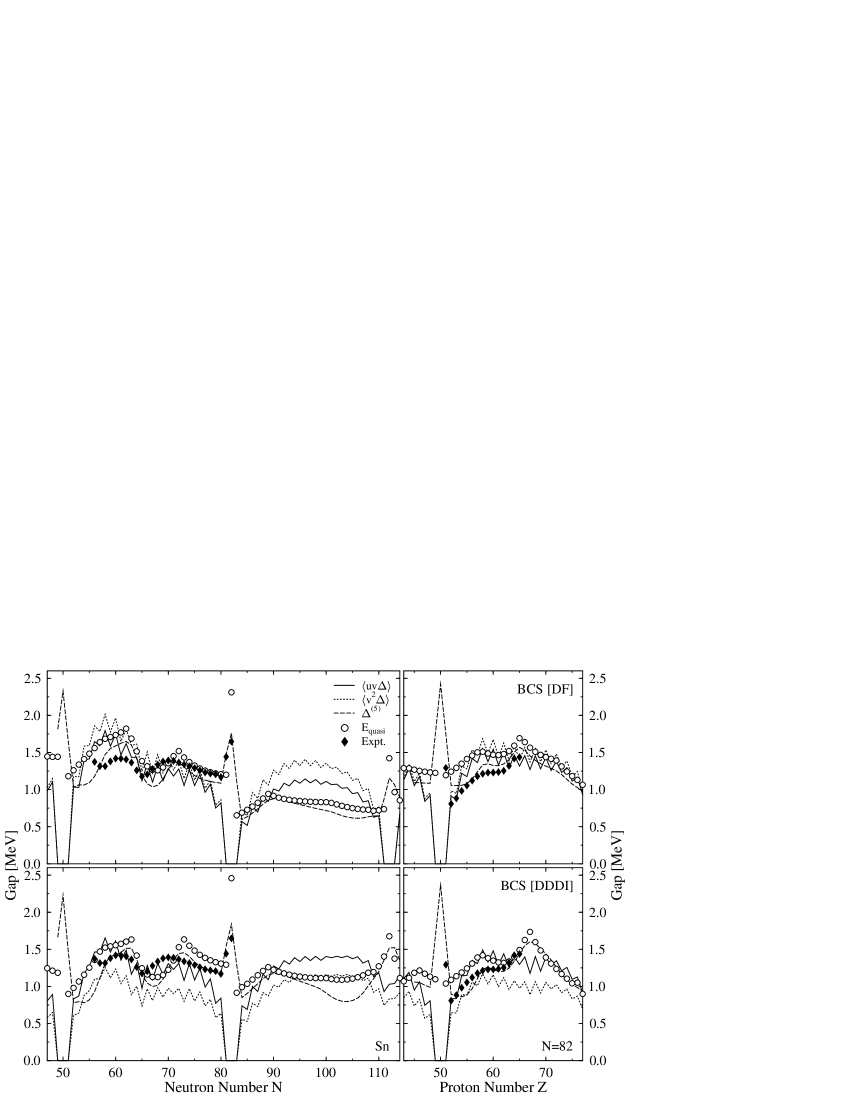
Figure 4: Comparison of the five–point gap $\Delta^{(5)}$, the spectral gap $\langle uv\Delta\rangle$, the average gap $\langle v^{2}\Delta\rangle$, and the single–quasiparticle energy $E_{\rm quasi}$ with experimental values for the five–point gap for tin isotopes (left panels) and $N=82$ isotones (right panels) calculated with a delta pairing force (upper panels) and DDDI force (lower panels) in the BCS scheme. The experimental values are calculated from the binding energies given in Wapstra using the five–point formula $\Delta^{(5)}$ (26).

Having discussed the various finite difference gaps, we now take the five–point gap as reference value and study the relation to the spectral gaps and quasiparticle energies. Figure 4 compares calculated results for $\Delta^{(5)}$, $\langle v^{2}\Delta\rangle$, $\langle uv\Delta\rangle$ and $E_{\rm quasi}$ computed within the BCS approach.

Let us start the discussion by looking at the neutron gaps in the chain of tin isotopes calculated with the DF pairing interaction in the BCS approach (upper left panel). The spectral gaps $\langle uv\Delta\rangle$ and $\langle v^{2}\Delta\rangle$ show a pronounced odd–even staggering where the gaps of even–even nuclei have larger values than those of odd–mass nuclei. This is caused by the blocking of one state with a large weight $uv$ in the odd–mass nucleus. The blocked state does not contribute to the pairing potential, leading to overall smaller single–particle gaps (14). The amplitude of the odd–even staggering decreases, of course, with increasing neutron number $N$ because the relative contribution of a particular state to the pair density becomes smaller with increasing level density in the heavier isotopes.

Both $\langle v^{2}\Delta\rangle$ and $\langle uv\Delta\rangle$ are exactly zero for closed shell nuclei, i.e. $N=50$, $N=82$, $N=112$, and the adjacent odd mass–number nuclei. In these nuclei the BCS scheme breaks down. This is a deficiency of the BCS scheme which is related to the particle–number uncertainty of the BCS state Ringbook .

The quasiparticle energies $E_{\rm quasi}$ show a similar dependence on the neutron number as the $\Delta^{(5)}$, but for most nuclei they are 100–250 keV larger (and thus the same amount larger with respect to the $\Delta^{({\rm b})}$). This is caused by calculating the blocked many–body wave function entering $E_{\rm quasi}$ not self–consistently. The variational principle behind the self–consistent calculation of the odd–mass nuclei entering the $\Delta^{(5)}$ leads always to larger a binding energy of the odd–mass nuclei, lowering the calculated gap.

The quasiparticle energies show the same peak at shell closures as the finite–difference gaps which is again related to a spurious contribution from the mean field. For non–magic nuclei the lowest single–quasiparticle state usually corresponds to a single–particle state with $\epsilon_{k}^{\prime}\approx\lambda_{q}$ leading to the single–quasiparticle energy $E_{\rm quasi}\approx\Delta_{k}+\lambda_{2,q}$. In magic nuclei one has an additional contribution from the first term in the square root in Eq. (28) since the Fermi energy is approximately in the middle of the gap in the single–particle spectrum (In the BCS scheme, where the pairing breaks down for closed–shell nuclei the derivation of Eq. (28) is not valid. Then one has different Fermi energies for the removal and addition of a particle, which are the single–particle energies of the last occupied and first unoccupied single–particle state respectively). The large jump in the Fermi energy is the reason for the kink in the systematics of binding energies at shell closures, which in turn causes the peak in the finite–difference gaps discussed above.

While all definitions of the gap give similar values in the valley of stability, there appear large differences between the $\Delta^{(5)}$ and $E_{\rm quasi}$ on one hand and the $\langle v^{2}\Delta\rangle$ and $\langle uv\Delta\rangle$ on the other hand for neutron–rich nuclei beyond the $N=82$ shell closure. The spectral gaps overestimate the $\Delta^{(5)}$ (which closely follow the $\Delta^{({\rm b})}$ as discussed earlier). The $\langle uv\Delta\rangle$ are smaller than the $\langle v^{2}\Delta\rangle$ for all tin isotopes and in most systems the $\langle uv\Delta\rangle$ are closer to the $\Delta^{(5)}$ than the $\langle v^{2}\Delta\rangle$.

Now we want to look at the changes when employing the DDDI pairing functional instead of the simpler delta force, see the lower left panel of Fig. 4. There are two significant differences to the results obtained with the DF functional: (i) all gaps except $\langle v^{2}\Delta\rangle$ are larger by roughly $20\,\%$ for neutron–rich nuclei with $N>82$, and (ii) the $\langle v^{2}\Delta\rangle$ are always much smaller than the $\langle uv\Delta\rangle$. This trend is just the opposite from the one for the DF functional. This is caused by the different choice of weights in the definition of $\langle v^{2}\Delta\rangle$ and $\langle uv\Delta\rangle$ in combination with the spectral distribution of the single–particle gaps $\Delta_{k}$. While the DF pairing potential follows roughly the nuclear density distribution, the DDDI functional gives a pairing potential which is sharply peaked at the nuclear surface, see Fig. 5. This leads in case of the DF interaction to single–particle gaps $\Delta_{k}$ of comparable size for all bound states while in case of the DDDI interaction the $\Delta_{k}$ of deeply bound single–particle states are rather small, see the middle panel of Fig. 6. Together with the weight factors used to calculate $\langle uv\Delta\rangle$ and $\langle v^{2}\Delta\rangle$ – see the upper panel in Fig. 6 – this gives the observed pattern for the spectral gaps: when calculated with the DF interaction they are rather insensitive to the choice for the weight factors while there is a huge difference in case of the DDDI interaction.

Figure 5: Local pairing potential $\Delta(r)$ of the neutrons in ${}^{124}{\rm Sn}$ for the DF and DDDI pairing functionals. The DF pairing potential acts over the whole volume of the nucleus, while the DDDI pairing potential is peaked at the nuclear surface.

This explains also why the $\Delta^{(5)}$ extrapolate quite differently when comparing DF and DDDI pairing for neutron–rich nuclei. In these nuclei the states at the Fermi surface are only loosely bound and therefore have a large spatial extension but only small overlap with the volume–like DF pairing potential. An extreme example is the tin isotope with $N=112$ where DF pairing breaks down but DDDI pairing is still fully active. Experimental data on the excitation spectra of neutron–rich nuclei will give in the future valuable information to distinguish between volume–like (DF) and surface–peaked pairing interactions.

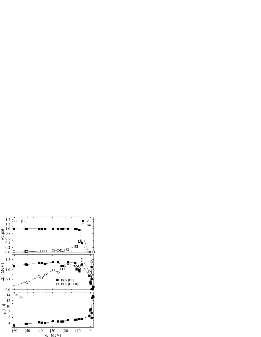
Figure 6: Weights $v^{2}$ (full diamonds) and $2uv$ (open diamonds) entering the calculation of the spectral gaps $\langle v^{2}\Delta\rangle$ and $\langle uv\Delta\rangle$ (upper panel), single–particle gap $\Delta_{k}$ in MeV (middle panel) and single–particle root–mean–square radius (lower panels) of the neutrons in ${}^{124}{\rm Sn}$, calculated with SkI4 in the BCS scheme. Weights and radii are shown for results with the DF functional only (DDDI gives very similar results), while the $\Delta_{k}$ are shown for the DF (diamonds) and DDDI (circles) pairing functionals. The horizontal line in the lower panel is the root–mean–square radius of the neutron density. The $uv$ in the upper panel are multiplied by two to have the same possible maximum value of one as the $v^{2}$.

This different behavior of $\langle v^{2}\Delta\rangle$ on one hand and $\langle uv\Delta\rangle$ and $\Delta^{(5)}$ on the other hand hints that is possibly dangerous to use different definitions of the gap for experimental and calculated gaps when fitting the pairing strength and comparing calculated and experimental values.

The right panels of Fig. 4 show the pairing gaps of the protons in the chain of $N=82$ isotones. Qualitatively the results are similar to those for the neutron gaps in the tin isotopes. But the overall reproduction of the experimental values is much better than in the case of tin isotopes and the differences between the various gaps is much smaller when going towards the drip–line. The Coulomb potential stabilizes even loosely–bound protons. Therefore the difference between the gaps comparing volume–like and surface–like pairing potentials is quite small. Only for the DDDI force remains the large difference between the spectral gaps $\langle v^{2}\Delta\rangle$ and $\langle uv\Delta\rangle$ explained above.

4.4 Lipkin–Nogami Pairing

Figure 7: Comparison of the five–point gap $\Delta^{(5)}$, the spectral gap $\langle uv\Delta\rangle$, the particle-number corrected spectral gap $\langle uv\Delta\rangle+\lambda_{2}$ and the single–quasiparticle energy $E_{\rm quasi}$ with experimental values for the five–point gap for tin isotopes (left panels) and $N=82$ isotones (right panels) calculated with a delta pairing force (upper panels) and DDDI force (lower panels) in the LN scheme.

Figure 7 shows the gaps of the neutrons in the chain of tin isotopes, now calculated with the LN scheme. The spectral gaps $\langle v^{2}\Delta\rangle$ are omitted here. Instead we compare the “bare” $\langle uv\Delta\rangle$ (30) with the particle–number corrected values $\langle uv\Delta\rangle+\lambda_{2}$ (32).

The global pattern of the various gaps looks very similar to the one obtained with the BCS scheme, see Fig. 4. The most obvious difference between the BCS and LN methods is that the LN scheme does not break down for closed–shell nuclei. Therefore the “bare” spectral gap $\langle uv\Delta\rangle$ has a finite – but still somewhat too small – value around magic nuclei. Adding $\lambda_{2}$ gives better results around shell closures, but away from shell closures the difference between $\langle uv\Delta\rangle$ and $\langle uv\Delta\rangle+\lambda_{2}$ for the tin isotopes is too small to decide on one preferred definition.

From the difference between $\langle uv\Delta\rangle$ and $\langle uv\Delta\rangle+\lambda_{2}$ it can be seen that $\lambda_{2}$ is largest around shell closures. But this indicates also that the LN approximation might not be sufficient for magic nuclei, a variational calculation of $\lambda_{2}$ or even full projection of the many–body wave function is needed Dob92a there.

The single–quasiparticle energies $E_{\rm quasi}$ follow closely the particle–number projected $\langle uv\Delta\rangle_{\rm p}+\lambda_{2,\rm p}$, which is easily understood remembering that $\lambda_{2}$ is added to both quantities. At shell closures, however, the single–quasiparticle energies overestimate the experimental gaps. Like in the case of the BCS scheme the $E_{\rm quasi}$ are nearly always larger than the calculated five–point gaps $\Delta^{(5)}$.

4.5 Comparison of all Models

Figure 8: Comparison of the $\Delta^{(5)}$ calculated in the different pairing schemes for the chains of tin isotopes and $N=82$ isotones.

Finally, we want to compare the four pairing models, i.e. any combination of BCS or LN and DF or DDDI pairing. The comparison is done with respect to the five–point gap $\Delta^{(5)}$, which we prefer as the most robust empirical definition and which has turned out to be the most useful definition of the pairing gap. In Fig. 8 the five–point gaps calculated from various pairing schemes are compared with experimental values. The differences between BCS and LN are generally very small. It is to be remembered, however, that the effective pairing strength is readjusted for the LN scheme. The (approximate) particle–number projection increases the total binding energy, but this effect is renormalized by virtue of the fit delivering a slightly smaller pairing strength in the LN scheme. There is one detail where BCS and LN differ: the peak of $\Delta^{(5)}$ in the vicinity of closed shells is more spread out in case of LN which is probably due to the softening of the shell closure by LN.

The differences between the pairing forces (DF versus DDDI) are much larger. For the neutron gaps of tin isotopes close to the valley of stability and the proton gaps in the $N=82$ isotones all schemes and forces still give similar results, but large differences between the DF and DDDI force occur for neutron gaps around $N=60$ and very neutron–rich nuclei with $N>82$. Only the DDDI model can describe the gaps in both the light and heavy known tin isotopes, while the DF interaction overestimates the gaps in the light ones by up to 15–20$\%$. The particle–number projection has only a small effect on the gaps when the strength of the pairing interaction is readjusted. The better description of the tin isotopes around $N=60$ with the DDDI force gives a hint that this pairing interaction may be more realistic than a delta force. This, however, has to be taken with a grain of salt: it may also be a spurious effect due to a deficiency of the underlying mean–field. The disagreement between calculated and experimental $\Delta^{(5)}$ around $N=70$ is rather robust in that all forces and schemes give very similar results. For a profound decision which pairing interaction gives the most realistic results throughout the chart of nuclei more and other observables have to be investigated using various forces for the underlying mean–field. Research in that direction is underway.

We have checked that one obtains very similar results when comparing experimental and calculated three–point and four–point gaps. However, it is important that the experimental and calculated values are computed from the same formula. As already shown in Fig. 1, the various finite–difference formulae may give results which differ by $25\%$.

5 Summary

We have compared various approximations for the calculation of the pairing gap: three–point, four–point and five–point finite difference formulae where the gap is estimated from total binding energies of adjacent nuclei, spectral gaps with different weights which put bias on well–bound states or levels at the Fermi surface, and the single–quasiparticle energy. Predictions of four different pairing models for the gaps were compared, namely the BCS and LN pairing schemes employing the DF or DDDI interactions. Experimental values for the pairing gaps are usually calculated from a finite–difference formula. For the calculated gaps we find that apart from shell closures there are non–negligible deviations up to $25\%$ between the various definitions. Some definitions of the pairing gap cannot be used for closed–shell nuclei. Therefore, it is the safest choice to compute the pairing gaps from mean–field calculations in the same way as the experimental values.

The natural definition for the calculated gap is the difference in binding energy $\Delta^{({\rm b})}$ between the fully paired BCS ground state and the blocked one of odd–mass nuclei. The five–point gap $\Delta^{(5)}$ provides a reliable quantity to fit the effective pairing strength, among all approximations for the pairing gap it is closest to $\Delta^{({\rm b})}$. Therefore we use it to calculate the experimental pairing gaps and take it as point of reference for all other approximations for the pairing gap. Like the other finite–difference formulae $\Delta^{(5)}$ contains a spurious contribution from the mean field around magic numbers, which is related to the jump of the Fermi energy at shell closures.

The four–point gap $\Delta^{(4)}$ has nearly the same overall quality as the five–point gap as compared to $\Delta^{({\rm b})}$, but its definition has an ambiguity, so that we prefer the five–point gap. The three–point gap $\Delta^{(3)}$ has a large contribution from the mean–field, which becomes rather obvious looking at proton gaps, consequently this quantity should not be used for the fit of the pairing strength since deficiencies of the underlying mean–field (especially concerning the symmetry energy) may be visible in the $\Delta^{(3)}$. When comparing calculated and experimental $\Delta^{(3)}$ respectively $\Delta^{(4)}$ for a well–adjusted interaction, however, both gaps show the same quality like the five–point gaps $\Delta^{(5)}$.

In situations where it is not possible to calculate $\Delta^{(5)}$, e.g. looking at potential energy surfaces, a reasonable approximation for the pairing gap is provided by $\langle uv\Delta\rangle+\lambda_{2}$. By adding $\lambda_{2}$ to the spectral gap the approximate particle–number projection gives an improved reproduction of the calculated $\Delta^{(5)}$ in most cases. The spectral gap $\langle uv\Delta\rangle+\lambda_{2}$ is in much better agreement with the calculated $\Delta^{(5)}$ than the averaged gap $\langle v^{2}\Delta\rangle+\lambda_{2}$, which sets too much bias on deeply bound states and therefore should not be used in models in which the pairing interaction acts mainly at the nuclear surface. The single–quasiparticle energies always overestimate the $\Delta^{(5)}$, but this is not too surprising because they are calculated from a non–self–consistent wave function of the odd nucleus.

The results show the danger of comparing calculated and experimental gaps computed from different definitions. The deviations between the various definitions depend on the actual nucleus and become generally larger when going towards the drip–lines. This is important especially when adjusting the free parameters of the pairing interaction. Experimental and calculated gaps should be calculated in the same manner, the five–point gap provides a useful tool for that.

The choice of the test cases (heavy semi–magic nuclei) and restriction to spherical nuclei have minimized the impact of polarization effects on the gaps. Recent explorations of dynamical polarization effects Xu99a ; uggap hint that these may be non–negligible at a quantitative level. Conclusive answers are yet inhibited due to uncertainties of present mean–field models in the time–odd channel. This point deserves attention in future work.

Another open question is the functional form of the pairing interaction. We find in this paper that the DDDI functional gives a slightly better description of pairing gaps compared with a delta pairing force, but to give a definitive answer one has to look at more nuclei and other data as well. Work in this direction is underway.

Appendix A The calculation of ${\mathbf{\lambda}_{2}}$

A.1 The General Expression

In case of an underlying many–body Hamiltonian $\hat{H}$ the parameter $\lambda_{2}$ in the variational equation is fixed by the condition

$$\langle\hat{K}\hat{N}_{2}^{2}\rangle=0\quad,$$ (33)

where $\hat{K}$ is given by

$$\hat{K}=\hat{H}-\sum_{q\in p,n}\Big{(}\lambda_{1,q}\langle\hat{N}_{q}\rangle+\lambda_{2,q}\langle\hat{N}_{q}^{2}\rangle\Big{)}$$ (34)

and $\hat{N}_{2}$ is the two–quasiparticle part of the particle–number operator (17). Because we look at like-particle pairing only the equations for protons and neutrons separate. Therefore the index $q$ for the isospin of the particle–number operator, the single–particle states etc can suppressed to get a compact notation. Introducing the shifted many–body state Rei96a

$$|\xi\rangle={\rm e}^{{\rm i}\xi\hat{N}_{2}}|0\rangle\qquad\hbox{with}\qquad|0\rangle=|\xi\rangle\Big{|}_{\xi=0}\quad,$$ (35)

the condition (33) is equivalent to

$$\partial_{\xi}^{2}\langle 0|\hat{K}|\xi\rangle\Big{|}_{\xi=0}=0\quad.$$ (36)

This can be resolved into an expression for $\lambda_{2}$

$$\lambda_{2}=\frac{\partial_{\xi}^{2}\langle 0|\hat{H}|\xi\rangle\Big{|}_{\xi=0}}{\partial_{\xi}^{2}\langle 0|\hat{N}^{2}|\xi\rangle\Big{|}_{\xi=0}}\quad.$$ (37)

The denominator of (37) can be calculated easily using Wick’s theorem

$$\partial_{\xi}^{2}\langle 0|\hat{N}^{2}|\xi\rangle\Big{|}_{\xi=0} = 8\Big{[}\sum_{k\gtrless 0}u_{k}^{2}v_{k}^{2}\Big{]}^{2}-16\sum_{k\gtrless 0}u_{k}^{4}v_{k}^{4}\quad.$$ (38)

So far we have formulated the numerator in terms of an underlying many–particle Hamiltonian, but the formulation (36) has the advantage that it can be translated into the formal framework of energy functionals Rei96a

$$\langle 0|\hat{H}|\xi\rangle\quad\Rightarrow\quad{\cal E}^{(\xi)}={\cal E}[\hat{\rho}^{(\xi)},\hat{\chi}^{(\xi)},\hat{\chi}^{*(\xi)}]\quad.$$ (39)

$\hat{\rho}^{(\xi)}$ and $\hat{\chi}^{(\xi)}$ are the shifted density matrix and pair density matrix respectively, which have to be calculated now as non-diagonal matrix elements

$$\hat{\rho}^{(\xi)} \equiv \rho^{(\xi)}(\vec{x},\vec{x}^{\prime})=\langle 0|\hat{\psi}^{\dagger}(\vec{x}^{\prime})\hat{\psi}(\vec{x})|\xi\rangle$$ (40a)

$$\hat{\chi}^{(\xi)} \equiv \chi^{(\xi)}(\vec{x},\vec{x}^{\prime})=-\sigma^{\prime}\langle 0|\hat{\psi}(\vec{r}^{\prime},-\sigma^{\prime})\hat{\psi}(\vec{x})|\xi\rangle$$ (40b)

$$\hat{\chi}^{*(\xi)} \equiv \chi^{*(\xi)}(\vec{x},\vec{x}^{\prime})=-\sigma\langle 0|\hat{\psi}^{\dagger}(\vec{x}^{\prime})\hat{\psi}^{\dagger}(\vec{r},-\sigma)|\xi\rangle$$ (40c)

All local densities and currents the Skyrme and pairing energy functionals depend on can be derived from these density matrices. The second derivative of the energy functional is given by

$$\partial_{\xi}^{2}{\cal E}^{(\xi)} = {\rm tr}\bigg{\{}\frac{\delta{\cal E}}{\delta\hat{\rho}}\partial^{2}_{\xi}\hat{\rho}+\frac{\delta{\cal E}}{\delta\hat{\chi}}\partial^{2}_{\xi}\hat{\chi}+\frac{\delta{\cal E}}{\delta\hat{\chi}^{*}}\partial^{2}_{\xi}\hat{\chi}^{*}\bigg{\}}$$ (41)

$$+{\rm tr}\,{\rm tr}\bigg{\{}\frac{\delta^{2}{\cal E}}{\delta\hat{\rho}_{1}\delta\hat{\rho}_{2}}\partial_{\xi}\hat{\rho}_{1}\,\partial_{\xi}\hat{\rho}_{2}+2\frac{\delta^{2}{\cal E}}{\delta\hat{\chi}\delta\hat{\chi}^{*}}\partial_{\xi}\hat{\chi}\,\partial_{\xi}\hat{\chi}^{*}$$

$$\quad+2\frac{\delta^{2}{\cal E}}{\delta\hat{\rho}\,\delta\hat{\chi}}\partial_{\xi}\hat{\rho}\,\partial_{\xi}\hat{\chi}+2\frac{\delta^{2}{\cal E}}{\delta\hat{\rho}\,\delta\hat{\chi}^{*}}\partial_{\xi}\hat{\rho}\,\partial_{\xi}\hat{\chi}^{*}\bigg{\}}\;.$$

$\delta$ stands for a functional derivative. The trace is a shorthand notation for the integration and summation over all coordinates

$${\rm tr}\left\{\frac{\delta{\cal E}}{\delta\hat{\rho}}\hat{\rho}\right\}\equiv\iint\!{\rm d}x\;{\rm d}x^{\prime}\;\frac{\delta{\cal E}}{\delta\rho(\vec{x},\vec{x}^{\prime})}\rho(\vec{x},\vec{x}^{\prime})\quad.$$ (42)

The terms with a single trace in (41) vanish in case of a BCS ground state, while the terms with double traces can be simplified defining the response density matrices $\tilde{\rho}$, $\tilde{\chi}$ and $\tilde{\chi}^{*}$

$$\tilde{\rho}=-{\rm i}\;\partial_{\xi}\,\hat{\rho}^{(\xi)}\Big{|}_{\xi=0}\quad,\quad\tilde{\chi}=-{\rm i}\;\partial_{\xi}\,\hat{\chi}^{(\xi)}\Big{|}_{\xi=0}\quad.$$ (43)

leading to the final expression

$$\partial^{2}_{\xi}{\cal E}^{(\xi)}\Big{|}_{\xi=0} = -{\rm tr}\,{\rm tr}\bigg{\{}\frac{\delta^{2}{\cal E}}{\delta\hat{\rho}_{1}\delta\hat{\rho}_{2}}\tilde{\rho}_{1}\,\tilde{\rho}_{2}+2\frac{\delta^{2}{\cal E}}{\delta\hat{\chi}\delta\hat{\chi}^{*}}\tilde{\chi}\,\tilde{\chi}^{*}$$ (44)

$$\quad+2\frac{\delta^{2}{\cal E}}{\delta\hat{\rho}\,\delta\hat{\chi}}\tilde{\rho}\,\tilde{\chi}+2\frac{\delta^{2}{\cal E}}{\delta\hat{\rho}\,\delta\hat{\chi}^{*}}\tilde{\rho}\,\tilde{\chi}^{*}\bigg{\}}$$

which has to be inserted into (37). Since we are considering pairing between like particles only there are no mixed terms with derivatives with respect to proton and neutron densities. This expression has to be evaluated now for the pairing and the mean–field energy functional. This density–functional approach to the calculation of $\lambda_{2}$ incorporates in a natural way the additional contributions to the LN equations arising for density–dependent interactions discussed in Val96a ; Val97a .

A.2 The Linear Response of a Skyrme Energy Functional

The Skyrme energy functionals are constructed to be effective interactions for nuclear mean–field calculations. For even–even nuclei, the Skyrme energy functional used in this paper

$${\cal E}={\cal E}_{\rm kin}+{\cal E}_{\rm Sk}+{\cal E}_{\rm C}\quad,$$ (45)

is the sum of the functional of the kinetic energy ${\cal E}_{\rm kin}$, the effective functional for the strong interaction ${\cal E}_{\rm Sk}$ and the Coulomb interaction ${\cal E}_{\rm C}$ including the exchange term in Slater approximation. The actual functionals are given by

$${\cal E}_{\rm kin} = \frac{\hbar^{2}}{2m}\int\!{\rm d}^{3}r\;\tau\quad,$$

$${\cal E}_{\rm C} = \frac{e^{2}}{2}\!\!\iint\!{\rm d}^{3}r\,{\rm d}^{3}r^{\prime}\frac{\rho_{\rm p}(\textbf{r})\rho_{\rm p}(\textbf{r}^{\prime})}{|\textbf{r}-\textbf{r}^{\prime}|}-\frac{3e^{2}}{4}\!\left(\frac{3}{\pi}\right)^{1/3}\!\!\!\!\int\!{\rm d}^{3}r\,\rho_{\rm p}^{4/3}$$

$${\cal E}_{\rm Sk} = \int\!{\rm d}^{3}r\bigg{[}\frac{b_{0}}{2}\rho^{2}+b_{1}\rho\tau-\frac{b_{2}}{2}\rho\Delta\rho+\frac{b_{3}}{3}\rho^{\alpha+2}-b_{4}\rho\nabla\cdot{\bf{J}}$$ (46)

$$\quad-\sum_{q}\bigg{(}\frac{b^{\prime}_{0}}{2}\rho_{q}^{2}+b^{\prime}_{1}\rho_{q}\tau_{q}-\frac{b^{\prime}_{2}}{2}\rho_{q}\Delta\rho_{q}$$

$$\qquad\qquad+\frac{b^{\prime}_{3}}{3}\rho^{\alpha}\rho_{q}^{2}+b^{\prime}_{4}\rho_{q}\nabla\cdot{\bf J}_{q}\bigg{)}\bigg{]}\quad.$$

The local density $\rho_{q}$, kinetic density $\tau_{q}$ and spin–orbit current ${\bf J}_{q}$ entering the functional are given by

$$\rho_{q}(\vec{r}) = \sum_{\sigma=\pm}\rho_{q}(\vec{r},\sigma;\vec{r},\sigma)$$

$$= \sum_{k\in\Omega_{q}}v_{k}^{2}\;|\phi_{k}(\vec{r})|^{2}\quad,$$

$$\tau_{q}(\vec{r}) = \sum_{\sigma=\pm}{\bf\nabla}\cdot{\bf\nabla}{}^{\prime}\rho_{q}(\vec{r},\sigma;\vec{r}^{\prime},\sigma)\Big{|}_{\vec{r}=\vec{r}^{\prime}}$$

$$= \sum_{k\in\Omega_{q}}v_{k}^{2}\;|\nabla\phi_{k}(\vec{r})|^{2}\quad,$$

$${\bf J}_{q}(\vec{r}) = -{\textstyle\frac{{\rm i}}{2}}({\bf\nabla}-{\bf\nabla}^{\prime})\times\sum_{\sigma,\sigma^{\prime}=\pm}\rho_{q}(\vec{r},\sigma;\vec{r}^{\prime},\sigma^{\prime})\;\vec{\sigma}_{\sigma^{\prime}\sigma}\Big{|}_{\vec{r}=\vec{r}^{\prime}}$$ (47)

$$= -{\textstyle\frac{{\rm i}}{2}}\sum_{k\in\Omega_{q}}v_{k}^{2}\;\Big{[}\phi_{k}^{\dagger}(\vec{r})\,\nabla\times\hat{\sigma}\,\phi_{k}(\vec{r})-\mbox{ h.c. }\Big{]}\;,$$

with $q\in\{{\rm p,n}\}$. $\vec{\sigma}_{\sigma^{\prime}\sigma}$ is the matrix element of the vector of the Pauli spin matrices between the unit spinors with spin projection $\sigma^{\prime}/2$ and $\sigma/2$. Densities without index in (A.2) denote total densities, e.g. $\rho=\rho_{\rm p}+\rho_{\rm n}$. The $\phi_{k}$ are the spinors of the single–particle wave functions, the $v^{2}$ occupation probabilities. The parameters $b_{i}$ and $b^{\prime}_{i}$ used in the above definition are chosen to give a most compact formulation of the energy functional, the corresponding mean–field Hamiltonian and residual interaction Rei92 . The Skyrme energy functional contains an extended spin–orbit coupling with an explicit isovector degree–of–freedom as used in the parameterization SkI4 Rei95a .

The response densities needed for the evaluation of (44) are given by

$$\tilde{\rho}_{q} = 2\sum_{k\in\Omega_{q}}u_{k}^{2}v_{k}^{2}\;|\phi_{k}|^{2}\quad,$$

$$\tilde{\tau}_{q} = 2\sum_{k\in\Omega_{q}}u_{k}^{2}v_{k}^{2}\;|{\bf\nabla}\phi_{k}|^{2}\quad,$$

$$\tilde{\bf J}_{q} = -{\rm i}\sum_{k\in\Omega_{q}}u_{k}^{2}v_{k}^{2}\,\Big{[}\phi_{k}^{\dagger}\,\nabla\times\hat{\sigma}\,\phi_{k}-(\nabla\times\hat{\sigma}\,\phi_{k})^{\dagger}\phi_{k}\Big{]}\quad.$$

Evaluating Eq. (44) for the Skyrme energy functional (A.2) leads to

$$\partial^{2}_{\xi}{\cal E}_{\rm Sk}^{(\xi)}\Big{|}_{\xi=0}$$

$$= {\rm tr}\;{\rm tr}\bigg{\{}\tilde{\rho}_{q,1}\frac{\delta^{2}{\cal E}_{\rm Sk}}{\delta\rho_{q,1}\,\delta\rho_{q,2}}\;\tilde{\rho}_{q,2}+2\tilde{\rho}_{q}\;\frac{\delta^{2}{\cal E}_{\rm Sk}}{\delta\rho_{q}\,\delta\tau_{q}}\;\tilde{\tau}_{q}$$

$$\qquad+2\tilde{\rho}_{q}\;\frac{\delta^{2}{\cal E}_{\rm Sk}}{\delta\rho_{q}\,\delta{\bf J}_{q}}\cdot\tilde{\bf J}_{q}\bigg{\}}$$

$$= \int\!{\rm d}^{3}r\;\bigg{\{}\big{(}b_{0}-b_{0}^{\prime}\big{)}\tilde{\rho}_{q}^{2}+2\big{(}b_{1}-b_{1}^{\prime}\big{)}\tilde{\rho}_{q}\tilde{\tau}_{q}$$

$$\quad-\big{(}b_{2}-b_{2}^{\prime}\big{)}\tilde{\rho}_{q}\Delta\tilde{\rho}_{q}-2\big{(}b_{4}+b_{4}^{\prime}\big{)}\tilde{\rho}_{q}{\bf\nabla}\cdot\tilde{\bf J}_{q}\phantom{\Big{[}}$$

$$\quad+\tfrac{1}{3}\big{[}(\alpha+2)(\alpha+1)b_{3}-2b_{3}^{\prime}\big{]}\,\rho^{\alpha}\,\tilde{\rho}_{q}^{2}\phantom{\Big{[}}$$

$$\quad-b_{3}^{\prime}\tfrac{1}{3}\Big{[}4\alpha\rho^{\alpha-1}\,\rho_{q}+\alpha(\alpha-1)\rho^{\alpha-2}\sum_{q^{\prime}}\rho_{q^{\prime}}^{2}\Big{]}\,\tilde{\rho}_{q}^{2}\bigg{\}}\quad.$$

For the local densities appearing in (A.2) the trace reduces to a spatial integral. For the protons one has an additional contribution from the Coulomb interaction

$$\partial^{2}_{\xi}{\cal E}_{\rm C}^{(\xi)}\Big{|}_{\xi=0}$$ (49)

$$= {\rm tr}\,{\rm tr}\left\{\tilde{\rho}_{\text{p}}\,\frac{\delta^{2}{\cal E}_{\text{C}}}{\delta\rho_{\text{p}}\,\delta\rho_{\text{p}}}\;\tilde{\rho}_{\rm p}\right\}$$

$$= e^{2}\!\!\iint\!{\rm d}^{3}r\;{\rm d}^{3}r^{\prime}\,\frac{\tilde{\rho}_{\text{p}}({\bf r})\,\tilde{\rho}_{\text{p}}({\bf r}^{\prime})}{|{\bf r}-{\bf r}^{\prime}|}-\frac{e^{2}}{3}\left(\frac{3}{\pi}\right)^{\!\!1/3}\!\!\int\!{\rm d}^{3}r\,\frac{\tilde{\rho}_{\text{p}}{}^{2}}{\rho_{\text{p}}^{2/3}}$$

$$= \int\!{\rm d}^{3}r\;\tilde{\rho}_{\text{p}}\;\tilde{V}_{\text{coul}}-\frac{e^{2}}{3}\left(\frac{3}{\pi}\right)^{\!\!1/3}\!\!\int\!{\rm d}^{3}r\,\frac{\tilde{\rho}_{\text{p}}{}^{2}}{\rho_{\text{p}}^{2/3}}\quad.$$

Poisson’s equation for the response Coulomb potential

$$\Delta\tilde{V}_{\text{coul}}=-4\pi\;\tilde{\rho}_{\text{p}}\quad.$$ (50)

is solved numerically using the techniques explained in Coul . The kinetic energy gives no contribution to $\lambda_{2}$. We omit the contribution from the center–of–mass correction (and therefore the approximate particle–number correction of this term).

A.3 The Linear Response of the Pairing Energy Functional

For the calculation of the contribution of a pairing energy functional of type (4) to Eq. (44) the local response pair density $\tilde{\chi}_{q}$ is needed

$$\tilde{\chi}_{q}=-{\rm i}\;\partial_{\xi}\chi_{q}^{(\xi)}\Big{|}_{\xi=0}=-4\sum_{k\in\Omega_{q}\atop k>0}f_{k}^{2}\;u_{k}^{3}v_{k}\;|\phi_{k}|^{2}\quad.$$ (51)

The response pair density is not hermitian, the adjoint response pair density $\tilde{\chi}^{\ast}_{q}$ reads

$$\tilde{\chi}^{\ast}_{q}=-{\rm i}\;\partial_{\xi}\chi_{q}^{\ast(\xi)}\Big{|}_{\xi=0}=4\sum_{k\in\Omega_{q}\atop k>0}f_{k}^{2}\;u_{k}v_{k}^{3}\;|\phi_{k}|^{2}\quad.$$ (52)

In case of the DF pairing energy functional there is only one contribution from the derivatives with respect to the pair density (44)

$$\partial^{2}_{\xi}{\cal E}_{\rm DF}^{(\xi)}\Big{|}_{\xi=0} = 2\,{\rm tr}\,{\rm tr}\left\{\tilde{\chi}_{q}\;\frac{\delta^{2}{\cal E}_{\rm DF}}{\delta\chi_{q}\,\delta\chi^{\ast}_{q}}\;\tilde{\chi}^{\ast}_{q}\right\}$$ (53)

$$= \frac{V_{q}}{2}\int\!{\rm d}^{3}r\;\tilde{\chi}_{q}^{\ast}\;\tilde{\chi}_{q}\quad.$$

In case of the DDDI pairing energy functional there are additional contributions from derivatives with respect to the local density

$$\partial^{2}_{\xi}{\cal E}_{\rm DDDI}^{(\xi)}\Big{|}_{\xi=0}$$ (54)

$$= {\rm tr}\,{\rm tr}\bigg{\{}2\tilde{\chi}_{q}\,\frac{\delta^{2}{\cal E}_{\text{\rm DDDI}}}{\delta\chi_{q}\,\delta\chi^{\ast}_{q}}\,\tilde{\chi}^{\ast}_{q}+2\tilde{\rho}_{q}\,\frac{\delta^{2}{\cal E}_{\text{\rm DDDI}}}{\delta\rho_{q}\,\delta\chi_{q}}\,\tilde{\chi}_{q}$$

$$\quad+2\tilde{\rho}_{q}\,\frac{\delta^{2}{\cal E}_{\text{\rm DDDI}}}{\delta\rho_{q}\,\delta\chi^{\ast}_{q}}\,\tilde{\chi}^{\ast}_{q}+\tilde{\rho}_{q,1}\,\frac{\delta^{2}{\cal E}_{\text{\rm DDDI}}}{\delta\rho_{q,1}\,\delta\rho_{q,2}}\,\tilde{\rho}_{q,2}\bigg{\}}$$

$$= \frac{V_{q}}{2}\int\!{\rm d}^{3}r\;\bigg{\{}\tilde{\chi}_{q}^{\ast}\;\tilde{\chi}_{q}\Big{[}1-\left({\textstyle\frac{\rho}{\rho_{0}}}\right)^{\gamma}\Big{]}$$

$$\quad-\frac{\gamma}{\rho_{0}^{\gamma}}\;\tilde{\rho}_{q}\;\rho^{\gamma-1}\Big{(}\tilde{\chi}^{\ast}_{q}\;\chi_{q}+\chi^{\ast}_{q}\;\tilde{\chi}_{q}\Big{)}$$

$$\quad-\frac{\gamma(\gamma-1)}{2\rho_{0}^{\gamma}}\tilde{\rho}_{q}^{2}\;\rho^{\gamma-2}\chi^{\ast}_{q}\;\chi_{q}\bigg{\}}\quad.$$

Appendix B Single–Quasiparticle Energies

The single–quasiparticle energies are deduced from the non–self–consistent ansatz

$$|k\rangle=\hat{\alpha}^{\dagger}_{k}\,|{\rm BCS}\rangle=v_{k}\,\hat{a}^{\dagger}_{k}\prod_{m>0\atop m\neq k}(u_{m}+v_{m}\hat{a}^{\dagger}_{m}\hat{a}^{\dagger}_{\bar{m}})\;|0\rangle$$ (55)

for the blocked many–body wave function of the odd mass number nucleus EGIII ; Ringbook ; Nilssonbook . The single–particle wave functions of all states and the occupation probabilities of all unblocked states $m\neq k$ are taken from the self–consistent calculation of the BCS ground state. The normalization of $|k\rangle$ requires $v_{k}=1$, $u_{k}=v_{k}=v_{\bar{k}}=0$. Note that $|k\rangle$ does not yield the proper particle number of the excited state because the occupation of the blocked pair of states $(k,\bar{k})$ in the BCS ground state in general will differ from one.

The excitation energy $E_{k}$ of the lowest one–quasiparticle state is an approximation for the odd–even mass difference. To take the difference in particle number between the fully paired BCS state and $|k\rangle$ into account, $E_{k}$ has to be calculated from the difference of ${\cal K}$ given by (10) calculated for $|k\rangle$ and the BCS ground state. This leads to

$$E_{k}={\cal E}^{(k)}+\langle k|\hat{N}^{\prime}|k\rangle-{\cal E}^{(0)}-\langle\hat{N}^{\prime}\rangle$$ (56)

where we have introduced the abbreviation

$$\hat{N}^{\prime}=-\sum_{q\in\{{\rm p,n}\}}\Big{(}\lambda_{1,q}\hat{N}_{q}+\lambda_{2,q}\hat{N}^{2}_{q}\Big{)}\quad.$$ (57)

${\cal E}^{(0)}$ is the energy functional of the BCS ground state, while ${\cal E}^{(k)}$ is the energy functional evaluated for the one–quasiparticle state $|k\rangle$.

The expectation values of $\hat{N}^{\prime}$ are conveniently calculated with standard operator techniques EGIII ; Ringbook ; Nilssonbook

$$\langle k|\hat{N}^{\prime}|k\rangle=\langle\hat{\alpha}^{\mbox{}}_{k}\hat{N}^{\prime}\;\hat{\alpha}^{\dagger}_{k}\rangle=\hat{N}_{00}^{\prime}+\langle\hat{\alpha}^{\mbox{}}_{k}\hat{N}_{11}^{\prime}\hat{\alpha}^{\dagger}_{k}\rangle\quad,$$ (58)

where $\hat{N}_{00}^{\prime}$ is the BCS expectation value of $\hat{N}^{\prime}$ while $\hat{N}_{11}^{\prime}$ is its (11) component. The Bogolyubov transformation of the particle–number operator reads

$$\hat{N} = \sum_{k\gtrless 0}\hat{a}^{\dagger}_{k}\hat{a}^{\mbox{}}_{k}$$ (59)

$$= \sum_{k\gtrless 0}\Big{[}v_{k}^{2}+(u_{k}^{2}-v_{k}^{2})\hat{\alpha}^{\dagger}_{k}\hat{\alpha}^{\mbox{}}_{k}+u_{k}v_{k}(\hat{\alpha}^{\dagger}_{k}\hat{\alpha}^{\dagger}_{\bar{k}}+\hat{\alpha}^{\mbox{}}_{\bar{k}}\hat{\alpha}^{\mbox{}}_{k})\Big{]}$$

$$= \hat{N}_{00}+\hat{N}_{11}+\hat{N}_{20}+\hat{N}_{02}\quad.$$

$(\hat{N}^{2})_{11}$ can be calculated from (59) without repetition of the quasiparticle transformation. One obtains

$$(\hat{N}^{2})_{11}=\sum_{k\gtrless 0}\Big{\{}(u_{k}^{2}-v_{k}^{2})[2(N+1)-4v_{k}^{2}]-1\Big{\}}\hat{\alpha}^{\dagger}_{k}\hat{\alpha}^{\mbox{}}_{k}\quad.$$ (60)

The calculation of the contribution of a many–body Hamiltonian operator to $E_{k}$ can be found in many textbooks, see e.g. EGIII ; Ringbook ; Nilssonbook . Here, however, we want to calculate it in the framework of effective energy functionals. The energy functional ${\cal E}^{(k)}={\cal E}[\hat{\rho}^{(k)},\chi^{(k)},\chi^{*(k)}]$ of the one–quasiparticle state is to be calculated from the density matrix and pair density matrix evaluated for the one–quasiparticle state $|k\rangle$

$$\rho^{(k)}(\vec{x};\vec{x}^{\prime})=\langle k|\hat{\psi}^{\dagger}(\vec{x}^{\prime})\hat{\psi}(\vec{x})|k\rangle\phantom{\sum_{m>0}}$$ (61a)

$$= \phi^{*}_{k}(\vec{x}^{\prime})\phi_{k}(\vec{x})+\sum_{m>0\atop m\neq k}v_{m}^{2}\;\phi^{*}_{m}(\vec{x}^{\prime})\,\phi_{m}(\vec{x})\quad,$$

$$\chi^{(k)}(\vec{r})=-\sum_{\sigma=\pm}\sigma\langle k|\hat{\psi}(\vec{r},-\sigma)\hat{\psi}(\vec{x})|k\rangle$$ (61b)

$$= -2\sum_{m>0\atop m\neq k}f_{m}u_{m}v_{m}|\phi(\vec{r})|^{2}\quad.$$

$\rho^{(k)}(\vec{x};\vec{x}^{\prime})$ and $\chi^{(k)}(\vec{r})$ are inserted into the definition of the energy functionals (45) and (4). This leads to

$$E_{k}={\cal E}^{(k)}-{\cal E}^{(0)}-(\lambda_{q}-4\lambda_{2,q}v_{k}^{2})(u_{k}^{2}-v_{k}^{2})+\lambda_{2,q}$$ (62)

where $\lambda_{q}=\lambda_{1,q}+4\lambda_{2,q}(N_{q}+1)$ was used.

The usual approximation for the one–quasiparticle energy is obtained taking only the linear change in the densities into account

$${\cal E}^{(k)}\approx{\cal E}^{(0)}+{\rm tr}\left\{\frac{\delta{\cal E}}{\delta\hat{\rho}}\delta\hat{\rho}+\frac{1}{2}\frac{\delta{\cal E}}{\delta\chi}\delta\chi+\frac{1}{2}\frac{\delta{\cal E}}{\delta\chi^{*}}\delta\chi^{*}\right\}$$ (63)

with

$$\delta\hat{\rho} = \hat{\rho}^{(k)}-\hat{\rho}=(1-2v_{k}^{2})\;\phi^{*}_{k}(\vec{x}^{\prime})\;\phi_{k}(\vec{x})\quad,$$ (64a)

$$\delta\chi = \delta\chi^{*}=\chi^{(k)}-\chi=2\,u_{k}v_{k}\;|\phi_{k}|^{2}\quad.$$ (64b)

This yields

$${\cal E}^{(k)}-{\cal E}^{(0)}\approx\epsilon_{k}(u_{k}^{2}-v_{k}^{2})+2f_{k}\Delta_{k}u_{k}v_{k}\quad.$$ (65)

Together with the contributions from the particle–number operators, Eqns. (59) and (60), one obtains

$$E_{k} = (\epsilon_{k}^{\prime}-\lambda_{q})\;(u_{k}^{2}-v_{k}^{2})+2f_{k}\Delta_{k}\;u_{k}v_{k}+\lambda_{2}$$ (66)

$$= \sqrt{(\epsilon^{\prime}_{k}-\lambda_{q})^{2}+f_{k}^{2}\Delta_{k}^{2}}+\lambda_{2,q}\quad,$$

where the definitions of the Fermi energy (12), the renormalized single–particle energy (13) and the expressions for $v_{k}^{2}$ and $u_{k}^{2}=1-v_{k}^{2}$ have been inserted.

References

- (1) J. Bardeen, L. N. Cooper, and J. R. Schrieffer, Phys. Rev. 108, 1175, (1957).
- (2) Å. Bohr, B. R. Mottelson, and D. Pines, Phys. Rev. 110, 936, (1958).
- (3) S. T. Belyaev, K. Dan. Vidensk. Selsk. Mat. Phys. Medd. 31, No. 11, (1958).
- (4) J. M. Eisenberg, and W. Greiner, Nuclear Theory Vol. III: Microscopic theory of the nucleus, North–Holland, Amsterdam, London, 1972.
- (5) P. Ring, and P. Schuck, The Nuclear Many–Body Problem, Springer, Heidelberg 1980.
- (6) S. G. Nilsson, and I. Ragnarsson, Shapes and Shells in Nuclear Structure, Cambridge University Press, Cambridge, 1995.
- (7) F. Tondeur, Nucl. Phys. A315, 353 (1979).
- (8) S. J. Krieger, P. Bonche, H. Flocard, P. Quentin, and M. S. Weiss, Nucl. Phys. A517, 275 (1990).
- (9) J. Dobaczewski, W. Nazarewicz, and T. R. Werner, Phys. Scr. T56, 15 (1995).
- (10) J. Dobaczewski, W. Nazarewicz, T. R. Werner, J. F. Berger, C. R. Chinn, and J. Dechargé, Phys. Rev. C 53, 2809 (1996).
- (11) J. Dechargé, and D. Gogny, Phys. Rev. C 21, 1568 (1980).
- (12) J. Dobaczewski, H. Flocard, and J. Treiner, Nucl. Phys. A422, 103 (1984).
- (13) H. J. Mang, Phys. Rep. 18, 325 (1975).
- (14) K. W. Schmid, and F. Grümmer, Rep. Prog. Phys. 50, 731 (1987).
- (15) H. J. Lipkin, Ann. Phys. (NY) 9, 272 (1960).
- (16) Y. Nogami, Phys. Rev. B134, 313 (1964).
- (17) H. C. Pradhan, Y. Nogami, and J. Law, Nucl. Phys. A201, 357 (1973).
- (18) H. Flocard, N. Onishi, Annals of Physics (NY) 254, 275 (1997).
- (19) D. C. Zheng, D. W. L. Sprung, and H. Flocard, Phys. Rev. C 46, 1355 (1992).
- (20) J. Dobaczewski and W. Nazarewicz, Phys. Rev. C 47, 2418 (1992).
- (21) P. Möller and J. R. Nix, Nucl. Phys. A536, 20 (1992).
- (22) P. Quentin, and H. Flocard, Ann. Rev. Nucl. Sci. 28, 523 (1978).
- (23) P.–G. Reinhard, Rep. Prog. Phys. 52, 439 (1989).
- (24) P.–G. Reinhard, and H. Flocard, Nucl. Phys. A584, 467 (1995).
- (25) P.–G. Reinhard, M. Bender, K. Rutz, and J. A. Maruhn, Z. Phys. A358, 277 (1997).
- (26) V. Blum, G. Lauritsch, J. A. Maruhn, and P.–G. Reinhard, J. Comp. Phys. 100, 364 (1992).
- (27) N. Tajima, P. Bonche, H. Flocard, P.–H. Heenen, and M. S. Weiss, Nucl. Phys. A551, 434 (1993).
- (28) S. A. Fayans, S. V. Tolokonnikov, E. L. Trybov, and D. Zawischa, Phys. Lett. B338, 1 (1994).
- (29) S. A. Fayans, and D. Zawischa, Phys. Lett. B383, 19 (1996).
- (30) D. G. Madland, and J. R. Nix, Nucl. Phys. A476, 1 (1988).
- (31) L. Bennour, P.–H. Heenen, P. Bonche, J. Dobaczewski, and H. Flocard, Phys. Rev. C 40, 2834 (1989).
- (32) W. Nazarewicz, M. A. Riley and J. D. Garrett, Nucl. Phys. A512, 61 (1990).
- (33) P. Quentin, N. Redon, J. Meyer, and M. Meyer, Phys. Rev. C 41, 341 (1990).
- (34) N. Tajima, P. Bonche, H. Flocard, P.–H. Heenen and M. S. Weiss, Nucl. Phys. A551, 409 (1993).
- (35) P.–H. Heenen, P. Bonche, J. Dobaczewski, and H. Flocard, Nucl. Phys. A561, 367 (1993).
- (36) J. Skalski, P.–H. Heenen, and P. Bonche, Nucl. Phys. A559, 221 (1993).
- (37) P. Magierski, P.–H. Heenen, and W. Nazarewicz, Phys. Rev. C 51, R2880 (1995).
- (38) P.–G. Reinhard, W. Nazarewicz, M. Bender, and J. A. Maruhn, Phys. Rev. C 53, 2776 (1996).
- (39) P. Magierski, S. Ćwiok, J. Dobaczewski, and W. Nazarewicz, Phys. Rev. C 48, 1686 (1993).
- (40) W. Satuła, R. Wyss, and P. Magierski, Nucl. Phys. A578, 45 (1994).
- (41) W. Satuła, R. Wyss, Phys. Rev. C 50, 2888 (1994).
- (42) B. Gall, P. Bonche, J. Dobaczewski, H. Flocard and P.–H. Heenen, Z. Phys. A348, 183 (1994).
- (43) R. Wyss and W. Satuła, Phys. Lett. B351, 393 (1995).
- (44) P.–H. Heenen, P. Bonche, and H. Flocard, Nucl. Phys. A588, 490 (1995).
- (45) J. Terasaki, P.–H. Heenen, P. Bonche, J. Dobaczewski, and H. Flocard, Nucl. Phys. A593 (1995), 1–20.
- (46) S. Ćwiok, J. Dobaczewski, P.–H. Heenen, P. Magierski, and W. Nazarewicz, Nucl. Phys. A611, 211 (1996).
- (47) A. Valor, J. L. Egido, and L. M. Robledo, Phys. Rev. C 53, 172 (1996).
- (48) A. Valor, J. L. Egido, and L. M. Robledo, Phys. Lett. 392B, 249 (1997).
- (49) K. Rutz, M. Bender, P.–G. Reinhard, J. A. Maruhn, and W. Greiner, Nucl. Phys. A634, 67 (1998).
- (50) J. Dobaczewski and J. Dudek, Phys. Rev. C 52, 1827 (1995), 55, 3177(E) (1997).
- (51) J. Engel, M. Bender, J. Dobaczewski, W. Nazarewicz, and R. Surman, Phys. Rev. C 60, 014302 (1999).
- (52) W. Satuła, J. Dobaczewski, and W. Nazarewicz, Phys. Rev. Lett. 81, 3599 (1998).
- (53) W. Satuła, Proceedings of the Nuclear Structure ’98 International Conference, Gatlinburg, Tennessee, U.S.A., August 10–15, 1998, C. Baktash [ed.], AIP Conference Proceedings 481, AIP, Woodbury, New York 1999, page 141.
- (54) R. R. Xu and R. Wyss, and P. M. Walker, Phys. Rev. C 60, 051301 (1999).
- (55) K. Rutz, M. Bender, P.–G. Reinhard, and J. A. Maruhn, Phys. Lett. B468, 1 (1999).
- (56) A. S. Jensen, P. G. Hansen, B. Jonson, Nucl. Phys. A431, 393 (1984).
- (57) Å. Bohr, and B. R. Mottelson, Nuclear Structure Vol I: Single–Particle Motion, World Scientific, Singapore, 1998.
- (58) G. Audi, and A. H. Wapstra, Nucl. Phys. A595, 409 (1995).
- (59) P.–G. Reinhard, Annalen der Physik (Leipzig) 1, 632 (1992).
- (60) J. A. Maruhn, T. A. Welton, and C. Y. Wong, Comput. Phys. 20, 326 (1976).