Abstract

We show that the tail of the chiral two-pion exchange nucleon-nucleon potential is proportional to the $\pi N$ scalar form factor and discuss how it can be translated into effective scalar meson interactions. We then construct a kernel for the process $NN\rightarrow\pi NN$, due to the exchange of two pions, which may be used in either three body forces or pion production in $NN$ scattering. Our final expression involves a partial cancellation among three terms, due to chiral symmetry, but the net result is still important. We also find that, at large internucleon distances, the kernel has the same spatial dependence as the central $NN$ potential and we produce expressions relating these processes directly.

PACS numbers: 13.75.Cs, 13.75.Gx, 11.30.Rd

1 Introduction

The description of pion production in nucleon-nucleon ($NN$) interactions near threshold is a traditional problem in hadron physics. In recent times the interest in it was renewed, due to a wealth of precise experimental data: $np\rightarrow d\pi^{0}$ [1], $pp\rightarrow pp\pi^{0}$ [2, 3], $pp\rightarrow d\pi^{+}$ [4, 5], $pp\rightarrow pn\pi^{+}$ [6]. On the theoretical side, the availability of chiral perturbation theory (ChPT) allowed the problem to be tackled in a systematic manner. However, in spite of all the effort made, a satisfactory picture is still not available.

There are two classes of interactions involved in this process, associated with either nucleon correlations or the emission of the external pion. In the procedure developed by Koltun and Reitan [7], these interactions are encompassed in wave functions and interaction kernels. The former correspond to solutions of the Schrödinger equation with realistic potentials, whereas the latter are described by models based on Feynman diagrams.

In the discussion of the production kernel, one usually distinguishes between long and short range contributions. The former are shown in Fig.1, where the first diagram represents the impulse approximation and the second, the pion rescattering term. These two processes were considered by Koltun and Reitan [7] in their description of the $\pi^{0}$ channel, but the corresponding cross section proved to underestimate recent data [1, 2, 3] by a factor 5 [8]. The rescattering term used in that work came from on shell $\pi N$ amplitudes, whereas the pion exchanged in diagram 1b is off-shell. Models which take pion virtuality into account enhances the cross section and tend to reduce underprediction [9, 10, 11, 12]. Heavy baryon ChPT calculations [13, 14, 15] also stressed the importance of this rescattering term at leading order. However, in these works the rescattering and impulse terms came out with opposite signs and the net result was again smaller than in phenomenological calculations [16]. Hence other mechanisms are needed to improve the description.

The next natural step concerns shorter range interactions, especially those involving two pions. The treatment of uncorrelated two-pion exchange is rather complex and, in the case of pion production, this part of the interaction has been described by effective heavy meson exchanges. Their contributions correspond to the last diagram of Fig.1, known as z-graph, since positive frequency nucleon propagation, already included in the wave function, is subtracted. The inclusion of $\sigma$, $\omega$ and $\rho$ mesons, either explicitly [12] or into a general axial current density [17] gave rise to good fits to the $pp\rightarrow pp\pi^{0}$ cross section at threshold. However, the study of relativistic effects in $\pi^{0}$ production [18] demonstrated that z-graph effects are small and hence heavy mesons in ChPT [13, 14] do not give rise to the required increase in cross sections. Extension to other channels ($\pi^{+}$ and $\pi^{-}$), with inclusion of nucleon resonances [15, 19, 20] also did not improve the situation.

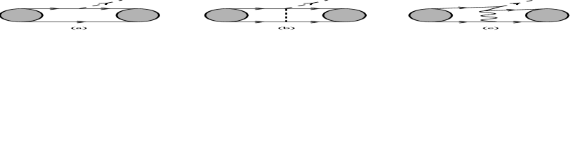
Figure 1: Contributions to the process $NN\rightarrow\pi NN$: (a) impulse, (b) rescattering and (c) z-graphs; nucleons, pions and heavier mesons are represented by solid, dashed and wavy lines.

Some time ago, Coon, Peña and Riska [21] produced a three-body potential based on the exchanges of a pion and a scalar meson, which proved to be able to reduce the gap between theory and experiment for the binding energy of trinuclei. Later on, we derived an equivalent result, using a non-linear Lagrangian, which included an effective chiral scalar meson coupled to nucleons [22]. In that work, the effective field was designed to simulate the two pion exchange potential. We stress that the exchange of two uncorrelated pions, formulated in the framework of chiral symmetry and including delta degrees of freedom, explains quite well the tail of the scalar-isoscalar nucleon-nucleon potential [23, 24, 25] and there is no need at all for a true scalar meson to describe that channel. On the other hand, the treatment of uncorrelated two pion exchange requires the calculation of many Feynman diagrams and, in problems where one is more concerned with simplicity than with fine details, it may be useful to replace all processes associated with the scalar-isoscalar channel by a single effective field. In this conceptual framework, our Lagrangian gave rise to a strong pion-scalar-nucleon contact interaction, that corresponds to the kernel for the reaction $NN\rightarrow\pi NN$ due to the exchange of two pions. This kernel was then applied to the $\pi^{0}$ and $\pi^{+}$ production channels and theoretical results were found to be comparable to the experimental ones [26]. Recently, calculations based on both relativistic [27] and heavy baryon ChPT [28] dealt with such a transition operator and large contributions were again found, involving several cancellations.

The purpose of the present work is two fold. In Sec.II, we discuss the relationship between the actual tail of the two-pion exchange potential and that provided by an effective scalar meson. The pion-production kernel is considered in Sec.III and, in order to determine the role of chiral cancellations, we study the leading term, constructed by means of the $\pi N\rightarrow\pi N$ and $\pi N\rightarrow\pi\pi N$ subamplitudes. Our results are indeed based on a partial cancellation, involving three large factors. We also find that, at large internucleon distances, the kernel has the same spatial dependence as the central $NN$ potential and hence, in Sec.IV, we produce expressions relating these interactions directly. Finally, in Sec.V we present a summary and conclusions.

2 Central Potential

The two-pion exchange potential (TPEP) is closely related to $\pi N$ scattering. The isoscalar amplitude for the process $NN\rightarrow NN$ is represented in Fig.2 and given by

$$\mathcal{T}^{S}\,=\,-\,\frac{i}{2!}\int\frac{d^{4}Q}{(2\pi)^{4}}\;\frac{3\;[T^{+}]^{(1)}\;[T^{+}]^{(2)}}{(k^{2}-\mu^{2})\,(k^{\prime\,2}-\mu^{2})}\;,$$ (1)

where $T^{+}$ is the isospin symmetric part of amplitude for the process $\pi^{a}N\rightarrow\pi^{b}N$ and $Q=(k^{\prime}+k)/2$.

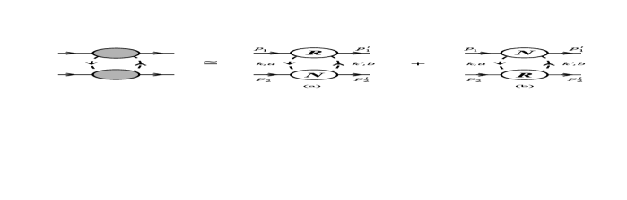
Figure 2: Leading contributions to the process $NN\rightarrow NN$.

In recent times, chiral symmetry has been systematically applied to this problem and one has learned [23, 24, 25] that it is convenient to separate $T^{+}$ into a contribution $T_{N}$, due only to pion-nucleon interactions, and a remainder $T_{R}$, involving other degrees of freedom. One then writes symbolically $[T^{+}]=[T_{N}^{+}]+[T_{R}^{+}]$ for each nucleon and the potential is then proportional to $[T^{+}]^{(1)}[T^{+}]^{(2)}=[T_{N}^{+}]^{(1)}[T_{N}^{+}]^{(2)}+\left\{[T_{N}^{+}]^{(1)}[T_{R}^{+}]^{(2)}+[T_{R}^{+}]^{(1)}[T_{N}^{+}]^{(2)}\right\}+[T_{R}^{+}]^{(1)}[T_{R}^{+}]^{(2)}$. The numerical study of these contributions has shown that the term within curly brackets is largely dominant [24] and due to the subamplitudes

$$T_{N}^{+} =\frac{g^{2}}{m}\;\bar{u}\,\left\{1-\left[\frac{m}{(p+k)^{2}-m^{2}}-\;\frac{m}{(p-k^{\prime})^{2}-m^{2}}\right]\,\!\!\not\!Q\right\}\,u\;,$$ (2)

$$T_{R}^{+} =\bar{A}^{+}(\nu=0,t=4\mu^{2})\;\bar{u}\,u=\frac{\alpha_{00}^{+}}{\mu}\;\bar{u}\,u\;,$$ (3)

where $g$ is the $\pi N$ coupling constant, $m$ is the nucleon mass and the bar over the isospin even $\pi N$ subamplitude $A^{+}$ indicates the subtraction of the pseudoscalar Born term. The constant $\alpha_{00}^{+}$ may be expressed as combination [24] of $\pi N$ subthreshold coefficients [29]. The leading contribution to $\mathcal{T}^{S}$ is written as

$$\mathcal{T}^{S}\;\cong\;3\,\frac{\alpha_{00}^{+}}{\mu}\;[\bar{u}\,u]^{(1)}\;\left[\Gamma_{N}^{+}\right]^{(2)}\;+\;\;(1\leftrightarrow 2)\;,$$ (4)

where

$$\left[\Gamma_{N}^{+}\right]^{(2)}=-\;\frac{i}{2}\int\frac{d^{4}Q}{(2\pi)^{4}}\;\frac{\left[T_{N}^{+}\right]^{(2)}}{[(Q\!-\!\Delta/2)^{2}\!-\!\mu^{2}]\;[(Q\!+\!\Delta/2)^{2}\!-\!\mu^{2}]}\;,$$ (5)

with $\Delta=(k^{\prime}-k)$. Using Eq.(2), we have

$$\left[\Gamma_{N}^{+}\right]^{(2)}=-\,\frac{i}{2}\,\frac{g^{2}}{m}\,\left\{\left[\bar{u}\,u\right]^{(2)}\int\frac{d^{4}Q}{(2\pi)^{4}}\;\frac{1}{[(Q\!-\!\Delta/2)^{2}\!-\!\mu^{2}]\;[(Q\!+\!\Delta/2)^{2}\!-\!\mu^{2}]}\right.$$

$$-\left.\left[\bar{u}\,\gamma_{\mu}\,u\right]^{(2)}\int\frac{d^{4}Q}{(2\pi)^{4}}\;\frac{2m\;Q^{\mu}}{[(Q\!-\!\Delta/2)^{2}\!-\!\mu^{2}]\;[(Q\!+\!\Delta/2)^{2}\!-\!\mu^{2}]\;[Q^{2}\!+\!2mV_{2}\!\cdot\!Q\!-\!\Delta^{2}/4]}\right\}$$

$$=\frac{1}{2}\,\frac{g^{2}}{m}\,\frac{1}{(4\pi)^{2}}\,\left[J_{c,c}(t)-J_{c,sN}^{(1)}(t)\right]\;\left[\bar{u}\,u\right]^{(2)}\,.$$ (6)

In deriving this result we used $V_{2}=(p_{2}^{\prime}+p_{2})/2m$ and the symmetry of the integrand under $Q\rightarrow-Q$. The functions $J$, defined in Ref.[30], are given by

$$J_{c,c}(t) =C(d,\Lambda)-\mu^{2}\int_{0}^{1}d\alpha\int_{0}^{1}\frac{d\beta}{\beta}\;\frac{\lambda^{2}}{t-\lambda^{2}\,\mu^{2}}\,,$$ (7)

$$J_{c,sN}^{(1)}(t) =-\,2m^{2}\int_{0}^{1}d\alpha\;\frac{1-\alpha}{\alpha}\int_{0}^{1}d\beta\;\frac{1-\beta}{\beta}\;\frac{1}{t-\eta^{2}\,\mu^{2}}\;,$$ (8)

with $t=\Delta^{2}$ and

$$\lambda^{2} =1/\left[\alpha(1-\alpha)\beta\right]\;,$$ (9)

$$\eta^{2} =\left[(1-\alpha)^{2}(1-\beta)^{2}\,m^{2}/\mu^{2}+1-(1-\alpha)(1-\beta)\right]\,/\,\left[\alpha(1-\alpha)\beta\right]\,.$$ (10)

The integral $J_{c,c}$ contains a function $C(d,\Lambda)$, where $d$ is the number of space-time dimensions and $\Lambda$ is the mass scale that arises in dimensional regularization. In the limit $d\rightarrow 4$ this function becomes divergent and needs to be removed by renormalization. We neglect this contribution because it has zero range and overlaps with other short distance effects not considered here.

The function $[\Gamma_{N}^{+}]$ is related to the scalar form factor $\sigma(t)$ by $\langle p^{\prime}|\mathcal{L}_{sb}|p\rangle=-\,\sigma(t)\,\left[\bar{u}\,u\right]$, where $\mathcal{L}_{sb}$ is the symmetry breaking Lagrangian. Its long range structure, as discussed by Gasser, Sainio and Švarc [31], is associated with diagrams 2a and 2b, and hence, in our notation, one has the equivalence

$$\sigma(t)\;[\bar{u}\,u]\;=\;3\,\mu^{2}\;[\Gamma_{N}^{+}]\;,$$ (11)

which is valid for large distances. This allows the asymptotic scalar potential to be written as

$$\mathcal{T}^{S}\;\cong\;2\,\frac{\alpha_{00}^{+}}{\mu}\,\frac{\sigma(t)}{\mu^{2}}\;[\bar{u}\,u]^{(1)}\;[\bar{u}\,u]^{(2)}\;.$$ (12)

This result is interesting because it sheds light into the structure of the interaction. The picture that emerges is that of a nucleon, acting as a scalar source, disturbing the pion cloud of the other. The function $\sigma(t)$ is related to the $\pi N$ $\sigma$-term by $\sigma(0)=\sigma_{N}$ and its value at the Cheng-Dashen point $t=2\mu^{2}$ may be extracted from experiment.

In some situations, it may be useful to use an effective parametrized version of $\sigma(t)$. In this case, the $t$ dependence of Eqs.(7-8) suggests that one should use the form

$$\sigma(t)\;\cong\;-\;\frac{c}{t-m_{s}^{2}}\;,$$ (13)

where the free parameters $c$ and $m_{s}$ may be written in terms of $\sigma(2\mu^{2})$ and $\sigma(0)$ as

$$c =\sigma(0)\;m_{s}^{2}\;,$$ (14)

$$m_{s}^{2} =\frac{2\;\sigma(2\mu^{2})}{\sigma(2\mu^{2})-\sigma(0)}\;\mu^{2}\,.$$ (15)

The coupling constant of this effective scalar state to nucleons may be obtained by comparing Eq.(12) with

$$\mathcal{T}^{S}\;\cong\;-\,\frac{g_{s}^{2}}{t-m_{s}^{2}}\;[\bar{u}\,u]^{(1)}\;[\bar{u}\,u]^{(2)}$$ (16)

and one has

$$g_{s}^{2}\;\cong\;2\,\alpha_{00}^{+}\;\frac{m_{s}^{2}\,\sigma(0)}{\mu^{3}}\;.$$ (17)

In Tab.1 we display the values of $g_{s}$ and $m_{s}$ obtained from input factors found in the recent literature. In most cases, the scalar mass is close to that used in the Bonn potential [35], but the coupling constant is smaller. We would like to stress, however, that the purpose of this exercise is not to predict theses values. Instead, it is to show that the actual asymptotic exchange of two uncorrelated pions may be naturally simulated in terms of an effective scalar interaction. As a final comment, one notes that the coupling constant given by Eq.(16) vanishes in the chiral limit and hence the effective approach is not equivalent to the linear $\sigma$-model, in which this does not happen.

Table 1: Predictions for $g_{s}$ and $m_{s}$ from Eqs. (14) and (15), using the following input parameters: $a\rightarrow\,$Ref.[29], $b\rightarrow\,$Ref.[31], $c\rightarrow\,$Ref.[32], $d\rightarrow\,$Ref.[33] and $e\rightarrow\,$Ref.[34].

$$\;\;\;\;\;\;\;\alpha_{00}^{+}\;\;\;\;\;\;\;$$ (MeV) (MeV) (MeV)

3.68 60 ^c 7.22 564

3.68 ^a 60 ^c 15 ^c 4.36 393

6.74 ^d 88 ^d 15 ^c 9.09 478

4.61 ^e 90 ^e 7.71 483

The non relativistic potential in configuration space is

$$V^{S}(x) =-\,2\,\alpha_{00}^{+}\;\frac{\mu}{4\pi}\left[\frac{4\pi}{\mu^{4}}\int\frac{d^{3}\Delta}{(2\pi)^{3}}\;e^{-i\,\mathbf{\Delta\,\cdot\,r}}\;\sigma(-\mathbf{\Delta}^{2})\right]$$

$$=-\,\left[3\,\alpha_{00}^{+}\;\frac{\mu}{m}\left(\frac{g}{4\pi}\right)^{2}\right]\,\frac{\mu}{4\pi}\,\left[S_{c,c}(x)-S_{c,sN}^{(1)}(x)\right]\;,$$ (18)

where $x=\mu\,r$ and

$$S_{c,c}(x) =\int_{0}^{1}d\alpha\int_{0}^{1}d\beta\;\frac{\lambda^{2}}{\beta}\;\frac{e^{-\lambda\,x}}{x}\;,$$ (19)

$$S_{c,sN}^{(1)}(x) =\frac{2m^{2}}{\mu^{2}}\int_{0}^{1}d\alpha\;\frac{1-\alpha}{\alpha}\int_{0}^{1}d\beta\;\frac{1-\beta}{\beta}\;\frac{e^{-\eta\,x}}{x}\;.$$ (20)

It is important to note that these functions $S$ are not of the Yukawa type and hence cannot be represented over their full range by terms proportional to $e^{-\,m_{s}\,r}/r$, irrespectively of the value chosen for the parameter $m_{s}$. In Fig.3 we display this potential together with that due to the exchange of an effective scalar meson.

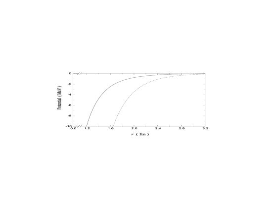
Figure 3: Scalar-isoscalar potential: asymptotic two-pion exchange (solid line), Eq.(18), and effective scalar exchange (dashed line), Eq.(16), with $\alpha_{00}^{+}=4.61$, $g_{s}=7.71$ and $m_{s}=483$ MeV taken from the last line of Tab.1.

3 The Kernel

In this section we construct a kernel for pion production in $NN$ scattering and due to the exchange of two pions. It is represented in Fig.4, denoted by $\mathcal{T}$ and based on $T_{cba}$ and $T_{ba}$, the amplitudes for the processes $\pi N\rightarrow\pi\pi N$ and $\pi N\rightarrow\pi N$, respectively. The kernel $\mathcal{T}$ for an outgoing pion with momentum $q$ and isospin index $c$ is

$$\mathcal{T}_{c}=-\,i\,\frac{1}{2!}\int\frac{d^{4}Q}{(2\pi)^{4}}\frac{T_{cba}\;T_{ba}}{(k^{2}-\mu^{2})(k^{\prime\,2}-\mu^{2})}\;.$$ (21)

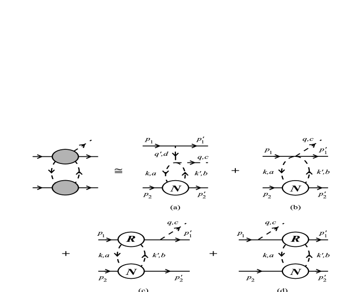
Figure 4: Contributions to the $NN\rightarrow\pi NN$ kernel: (a) pion-pole, (b) contact, (c) and (d) z-graphs.

The basic subamplitudes have the isospin structures

$$T_{ba} =\delta_{ab}\,T^{+}+i\,\epsilon_{bac}\tau_{c}\,T^{-}\;,$$ (22)

$$T_{cba} =-\,i\,\left\{\delta_{bc}\tau_{a}\,T_{A}+\delta_{ac}\tau_{b}\,T_{B}+\delta_{ab}\tau_{c}\,T_{C}+i\,\epsilon_{cba}\,T_{E}\right\}$$ (23)

and hence

$$\mathcal{T}_{c}=\tau_{c}^{(1)}\,\mathcal{T}_{1}+i\,(\mbox{\boldmath$\tau$}^{(1)}\times\mbox{\boldmath$\tau$}^{(2)})_{c}\,\mathcal{T}_{12}+\tau_{c}^{(2)}\,\mathcal{T}_{2}\;,$$ (24)

where

$$\mathcal{T}_{1} =-\;\frac{1}{2}\int\frac{d^{4}Q}{(2\pi)^{4}}\;\frac{\left[T_{A}+T_{B}+3\;T_{C}\right]^{(1)}\;\left[T^{+}\right]^{(2)}}{(k^{2}-\mu^{2})(k^{\prime\,2}-\mu^{2})}\;,$$ (25)

$$\mathcal{T}_{12} =-\;\frac{1}{2}\int\frac{d^{4}Q}{(2\pi)^{4}}\;\frac{\left[T_{A}-T_{B}\right]^{(1)}\;\left[T^{-}\right]^{(2)}}{(k^{2}-\mu^{2})(k^{\prime\,2}-\mu^{2})}\;,$$ (26)

$$\mathcal{T}_{2} =-\;\frac{1}{2}\int\frac{d^{4}Q}{(2\pi)^{4}}\;\frac{2\;\left[T_{E}\right]^{(1)}\;\left[T^{-}\right]^{(2)}}{(k^{2}-\mu^{2})(k^{\prime\,2}-\mu^{2})}\;.$$ (27)

We begin by discussing the process $\pi^{b}(k^{\prime})\,N(p)\rightarrow\pi^{a}(k)\,\pi^{c}(q)\,N(p^{\prime})$. The amplitude $T_{cba}$ is given by the sum of $T_{cba}^{\pi}$, a $t$-channel pion-pole contribution, and a remainder, denoted by $\bar{T}_{cba}$. The explicit forms of these terms, for a system containing just pions and nucleons, was presented in Ref.[36] and here we just quote the main results.

The pion-pole amplitude for on-shell nucleons is

$$i\,T_{cba}^{\pi}=-\;\frac{m\,g_{\mathrm{A}}}{f_{\pi}}\;\left[\bar{u}\,\tau_{d}\,\gamma_{5}\,u\right]\;\frac{T_{dcba}^{\pi\pi}}{(p^{\prime}\!-\!p)^{2}-\mu^{2}}\;,$$ (28)

where $f_{\pi}$ and $g_{\mathrm{A}}$ are the pion and axial decay constants, whereas $T_{dcba}^{\pi\pi}$ is the pion scattering amplitude. At tree level, it is given by

$$T_{dcba}^{\pi\pi}=\frac{1}{f_{\pi}^{2}}\;\left\{\delta_{ad}\delta_{bc}\left[(q\!-\!k^{\prime})^{2}\!-\!\mu^{2}\right]\!+\!\delta_{bd}\delta_{ac}\left[(q\!+\!k)^{2}\!-\!\mu^{2}\right]\!+\!\delta_{cd}\delta_{ab}\left[(k^{\prime}\!-\!k)^{2}\!-\!\mu^{2}\right]\right\}$$ (29)

and one has

$$T_{A}^{\pi}=-\;\frac{m\,g_{\mathrm{A}}}{f_{\pi}^{3}}\;\frac{(p^{\prime}\!-\!p\!+\!k)^{2}-\mu^{2}}{(p^{\prime}\!-\!p)^{2}-\mu^{2}}\;.$$ (30)

The evaluation of $\bar{T}_{cba}$ requires the calculation of a large number of diagrams. However, long ago Olsson and Turner [37] have shown that its leading contribution comes from the effective Lagrangian

$$\bar{\mathcal{L}}=\frac{g_{\mathrm{A}}}{8\,f_{\pi}^{3}}\;\bar{\psi}\,\gamma_{\mu}\,\gamma_{5}\,\mbox{\boldmath$\tau$}\,\psi\cdot\mbox{\boldmath$\phi$}\,\partial^{\mu}\mbox{\boldmath$\phi$}^{2}\;,$$ (31)

which gives the following contribution to $\bar{T}_{A}$

$$\bar{T}_{A}=\frac{2\,g_{\mathrm{A}}}{8\,f_{\pi}^{3}}\left(2m+\!\!\not\!k\right)\;.$$ (32)

The corresponding expressions for $T_{B}$ and $T_{C}$ are obtained by making $k\rightarrow-k^{\prime}$ and $k\rightarrow q$, respectively.

The main implication of this structure of the $\pi N\rightarrow\pi\pi N$ interaction for our study is that the leading contribution to $\mathcal{T}$ comes from the diagrams 4a and 4b. As the $NN$ interaction due to the exchange of two pions is dominated by the scalar-isoscalar channel, in this work we consider only the amplitude $\mathcal{T}_{1}$, Eq.(25), and postpone the discussion of the remaining components to another occasion.

Diagram 4a yields

$$\mathcal{T}_{1}^{\pi} =\left[\frac{m\,g_{\mathrm{A}}}{f_{\pi}^{3}}\right]\frac{1}{(p_{1}^{\prime}\!-\!p_{1})^{2}-\mu^{2}}\;[\bar{u}\,\gamma_{5}\,u]^{(1)}$$

$$\times\frac{1}{2}\int\frac{d^{4}Q}{(2\pi)^{4}}\;\frac{\left[2(p_{1}^{\prime}\!-\!p_{1})^{2}+2q\!\cdot\!\Delta+3\Delta^{2}/2-5\mu^{2}+2Q^{2}\right]\;\left[T^{+}\right]^{(2)}}{[(Q\!-\!\Delta/2)^{2}\!-\!\mu^{2}]\;[(Q\!+\!\Delta/2)^{2}\!-\!\mu^{2}]}\;.$$ (33)

We note that the last two terms in the result $Q^{2}=(\mu^{2}-\Delta^{2}/4)+[(Q\!-\!\Delta/2)^{2}\!-\!\mu^{2}]/2+[(Q\!+\!\Delta/2)^{2}\!-\!\mu^{2}]/2$ allow the cancellation of pion propagators and therefore correspond to short range effects that will be neglected here. We then obtain

$$\mathcal{T}_{1}^{\pi}=i\,\left[\frac{m\,g_{\mathrm{A}}}{f_{\pi}^{3}}\right]\,\left\{3+\frac{3q^{2}+4q\!\cdot\!(p_{1}^{\prime}\!-\!p_{1})}{(p_{1}^{\prime}\!-\!p_{1})^{2}-\mu^{2}}\right\}\,[\bar{u}\,\gamma_{5}\,u]^{(1)}\;\left[\Gamma_{N}^{+}\right]^{(2)}\,,$$ (34)

where $\left[\Gamma_{N}^{+}\right]^{(2)}$ is given by Eq.(5). This result may be associated with the scattering of a pion emitted in one of the nucleons by the pion cloud of the other, indicating that the kernel one is considering here is not fully disentangled from that usually called pion rescattering. Indeed, the description of the rescattering process is based on an intermediate $\pi N$ amplitude for off-shell pions, which satisfies a Ward-Takahashi identity [39]. In the isospin symmetric channel, this identity may be expressed as

$$T^{+}(q^{\prime\,2},q^{2})=T_{N}^{+}\;+\;\frac{q^{\prime\,2}+q^{2}-\mu^{2}}{f_{\pi}^{2}\,\mu^{2}}\;\sigma(t)\;[\bar{u}\,u]\;+\;r^{+}\;,$$ (35)

where $T_{N}^{+}$ is the nucleon pole (Born) term evaluated with pseudovector coupling, $q$ and $q^{\prime}$ are the momenta of the pions, $\sigma(t)$ is the scalar form factor and $r^{+}$ is a remainder that does not include leading order contributions.

The only term that depends strongly on off-shell effects is that proportional to the scalar form factor and hence one writes

$$T^{+}(q^{\prime\,2},q^{2})=T^{+}(\mu^{2},\mu^{2})+\delta T^{+}\,,$$ (36)

with

$$\delta T^{+}=\frac{(q^{\prime\,2}-\mu^{2})+(q^{2}-\mu^{2})}{f_{\pi}^{2}\,\mu^{2}}\;\sigma(t)\;[\bar{u}\,u]\;.$$ (37)

The contribution of this factor to the pion rescattering amplitude on nucleon 2 reads

$$\mathcal{T}_{1}^{\delta}=i\,\left[\frac{m\,g_{\mathrm{A}}}{f_{\pi}^{3}}\right]\,\left\{3+\frac{3(q^{2}-\mu^{2})}{(p_{1}^{\prime}-p_{1})^{2}-\mu^{2}}\right\}\,\left[\bar{u}\,\gamma_{5}\,u\right]^{(1)}\;\left[\Gamma_{N}^{+}\right]^{(2)}\,,$$ (38)

using Eq.(11). Adding this result to the on-shell $\pi N$ amplitude derived by Gasser, Sainio and Švarc, Ref.[31]-Eq.(A.35), one recovers Eq.(34). Therefore, in the sequence, we no longer consider the term proportional to the pion-pole in that expression, with the understanding that it should be included in the on-shell rescattering amplitude.

The evaluation of diagram 4b is more straightforward and produces

$$\bar{\mathcal{T}}_{1}=-\,i\,\left[\frac{m\,g_{\mathrm{A}}}{f_{\pi}^{3}}\right]\,\left[\bar{u}\,\left\{2+\frac{\!\!\not\!q}{2m}\right\}\,\gamma_{5}\,u\right]^{(1)}\,\left[\Gamma_{N}^{+}\right]^{(2)}\,.$$ (39)

Using the Goldberger-Treiman relation and Eq.(11), we have

$$\mathcal{T}_{1}^{\pi}+\bar{\mathcal{T}}_{1}=i\,\left[\frac{g}{3\mu^{2}f_{\pi}^{2}}\right]\sigma(t)\left[\bar{u}\,\left\{1-\;\frac{\!\!\not\!q}{2m}\right\}\,\gamma_{5}\,u\right]^{(1)}\,\left[\bar{u}\,u\right]^{(2)}\,.$$ (40)

One notes that when $\mathcal{T}_{1}^{\pi}$ and $\bar{\mathcal{T}}_{1}$ are added together, a cancellation occurs, which springs from the same mechanism and is very similar to that noticed long ago in the study of exchange currents in pion-deuteron scattering [38].

Another contribution with the same two-pion range comes from diagrams 4c and 4d, which yield

$$\mathcal{T}_{1}^{z}=i\,\left[\frac{g\,\alpha_{00}^{+}}{m\,\mu^{3}}\right]\,\sigma(t)\,\left[\bar{u}\,\left\{1-\;\frac{m\;\!\!\not\!q}{(p^{\prime}\!+\!q)^{2}-m^{2}}-\;\frac{m\;\!\!\not\!q}{(p\!-\!q)^{2}-m^{2}}\right\}\,\gamma_{5}\,u\right]^{(1)}\,\left[\bar{u}\,u\right]^{(2)}\,.$$ (41)

This result includes the propagation of positive energy states, that do not contribute to the kernel. Eliminating them and neglecting small non covariant terms, we have

$$\mathcal{T}_{1}^{z}=i\,\left[\frac{g\,\alpha_{00}^{+}}{m\,\mu^{3}}\right]\,\sigma(t)\,\left[\bar{u}\,\left\{1+\frac{\!\!\not\!q}{2m}\right\}\,\gamma_{5}\,u\right]^{(1)}\,\left[\bar{u}\,u\right]^{(2)}\,.$$ (42)

Our final expression for the covariant kernel is obtained by adding Eqs.(40) and (42) and reads

$$\mathcal{T}_{1}=i\,\sigma(t)\,g\,\left\{\left[\frac{1}{3\,\mu^{2}\,f_{\pi}^{2}}+\frac{\alpha_{00}^{+}}{m\,\mu^{3}}\right]\,\bar{u}\,\gamma_{5}\,u-\left[\frac{1}{3\,\mu^{2}\,f_{\pi}^{2}}-\frac{\alpha_{00}^{+}}{m\,\mu^{3}}\right]\,\bar{u}\,\frac{\!\!\not\!q}{2m}\,\gamma_{5}\,u\right\}^{(1)}\,\left[\bar{u}\,u\right]^{(2)}\,.$$ (43)

This covariant amplitude is our main result.

4 Application

In order to consider applications in low energy processes, we perform a non-relativistic approximations in our results. In the case of the central potential, Eq.(11), one has

$$t^{S}\,=\,2\,\alpha_{00}^{+}\,\sigma(t)\,/\,\mu^{3}\;,$$ (44)

where $t=-\,\mathbf{\Delta}^{2}$ and we have discarded a normalization factor $4m^{2}$. On the other hand, the kernel, suited to be used with nuclear wave functions, is

$$t_{1}=i\;\sigma(t)\;\frac{g}{2m}\left\{-\left[\frac{1}{3\,\mu^{2}\,f_{\pi}^{2}}+\frac{\alpha_{00}^{+}}{m\,\mu^{3}}\right]\mbox{\boldmath$\sigma$}\!\cdot\!(\mbox{\boldmath$p$}^{\prime}-\mbox{\boldmath$p$})+\left[\frac{1}{3\,\mu^{2}\,f_{\pi}^{2}}-\frac{\alpha_{00}^{+}}{m\,\mu^{3}}\right]\mbox{\boldmath$\sigma$}\!\cdot\!\mbox{\boldmath$q$}\right\}^{(1)}.$$ (45)

The term proportional to $\mbox{\boldmath$\sigma$}\!\cdot\!(\mbox{\boldmath$p$}^{\prime}-\mbox{\boldmath$p$})/3\mu^{2}f_{\pi}^{2}$ in this result coincides with that produced recently in Ref.[27].

As discussed in Refs.[21] and [22], a pion production kernel such as $t_{1}$ gives rise to three body forces and again one has $t\cong-\,\mathbf{\Delta}^{2}$. In the case of threshold pion production, on the other hand, $t\cong\mu^{2}/4-\mathbf{\Delta}^{2}$. In order to test the influence of these different values of $t$, in Fig.5 we plot the Fourier transform of the function $\sigma(t)$, that dictates the space dependence of the kernel in the two cases. Inspecting it, one learns that the energy component of the four momentum transferred has little importance and hence the static result also holds for the production kernel. This allows one to relate it directly to the central potential

$$t_{1}=i\,\frac{g_{\mathrm{A}}}{f_{\pi}}\,\frac{t^{S}}{2m}\left\{-\,\left[\frac{\mu\,m}{6\,\alpha_{00}^{+}\,f_{\pi}^{2}}+\frac{1}{2}\right]\,\mbox{\boldmath$\sigma$}\!\cdot\!(\mbox{\boldmath$p$}^{\prime}-\mbox{\boldmath$p$})+\left[\frac{\mu\,m}{6\,\alpha_{00}^{+}\,f_{\pi}^{2}}-\frac{1}{2}\right]\,\mbox{\boldmath$\sigma$}\!\cdot\!\mbox{\boldmath$q$}\right\}^{(1)}.$$ (46)

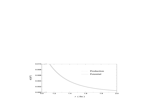
Figure 5: Fourier transform of $\sigma(t)$, that determine the space dependence of the three body force and production kernels, as function of the distance $r$.

In order to use these results in actual calculations, in either momentum or configuration spaces, one has to evaluate the function $\sigma(t)$ numerically and then, the sandwich of the kernel between two-nucleon wave functions. Since the kernel and the central potential are closely related, consistency would require that the same dynamics should be used in the construction of both the operator $t_{1}$ and the wave functions. However, at present, the potential due to the exchange of two pions is reliable at large distances only and hence it is not suited to determine wave functions by means of the Schrödinger equation. Therefore, the possibility of using Eq.(46) with ones favourite scalar potential is an interesting one.

5 Summary and Conclusions

In this work we have shown that the central component of the $NN$ potential at large distances, which is due to the exchange of two uncorrelated pions, may be naturally expressed in terms of $\sigma(t)$, the scalar form factor. This function is related to the $\pi N$ $\sigma$-term and may, if one wishes, be parametrized as an effective scalar meson exchange. However, the coupling of this state to nucleons vanishes in the chiral limit and hence this scalar meson does not correspond to that present in the linear $\sigma$-model.

We have also obtained a two-pion-exchange kernel for the process $NN\rightarrow\pi NN$, that can be applied in both three body forces and pion production in $NN$ scattering. The complete calculation of this kernel would require the evaluation of a large number of diagrams. Thus, in order to estimate the dominant contribution at large $NN$ distances, we have used just the leading contributions to the subamplitudes $\pi N\rightarrow\pi N$ and $\pi N\rightarrow\pi\pi N$, in the framework of chiral symmetry. The simplified result so obtained involves a cancellation between contact-three-pion and pion-pole vertices. The latter may also be associated with an off-shell intermediate $\pi N$ amplitude and has been include into the Tucson-Melbourne [40] two-pion exchange three nucleon potential. This means that this force does include a term describing a two-pion exchange between a pair of nucleons. Thus, the use of an on-shell $\pi N$ amplitude gives rise to a less ambiguous definition of the two-pion exchange three body force [41].

At large distances, the kernel is closely related to the two-pion exchange scalar isoscalar $NN$ potential. Indeed, in the case of three body forces, we could show that the kernel and the potential have the same spatial dependence. For threshold pion-production, this relationship is also approximately valid. These results led us to produce expressions that relate directly the kernel to the potential. Using the extreme numerical values for $\alpha_{00}^{+}$ found in the literature, namely 3.68 [29] and 6.74 [33], in Eq.(46), one has

$$t_{1}=\,i\;\frac{g_{\mathrm{A}}}{f_{\pi}}\,\frac{t^{S}}{2m}\left\{-\,1.18\,\mbox{\boldmath$\sigma$}\!\cdot\!(\mbox{\boldmath$p$}^{\prime}-\mbox{\boldmath$p$})+0.18\,\mbox{\boldmath$\sigma$}\!\cdot\!\mbox{\boldmath$q$}\right\}^{(1)}$$ (47)

or

$$t_{1}=\,i\;\frac{g_{\mathrm{A}}}{f_{\pi}}\,\frac{t^{S}}{2m}\left\{-\,0.87\,\mbox{\boldmath$\sigma$}\!\cdot\!(\mbox{\boldmath$p$}^{\prime}-\mbox{\boldmath$p$})-0.13\,\mbox{\boldmath$\sigma$}\!\cdot\!\mbox{\boldmath$q$}\right\}^{(1)}\,.$$ (48)

These results are quite close to the kernel obtained by ourselves sometime ago [22], given by

$$t_{1}=\,i\;\frac{g_{\mathrm{A}}}{f_{\pi}}\,\frac{t^{S}}{2m}\,\left\{-\,\mbox{\boldmath$\sigma$}\!\cdot\!(\mbox{\boldmath$p$}^{\prime}-\mbox{\boldmath$p$})\right\}^{(1)}\,,$$ (49)

in the case of a models based on effective scalar-isoscalar mesons. This allows one to consider the relationship between the kernel and the potential to be a rather general one. The reason for this generality springs from the old insight by Nambu [42] and Weinberg [43] that, for generic states $A$ and $B$, the leading contributions to the process $A\rightarrow\pi B$ are obtained by inserting the pion, with gradient coupling, into the external lines of the process $A\rightarrow B$.

Finally, we would like to point out that we may expect the contributions from the kernel $t_{1}$ to be large. In order to see this, note that momentum conservation allows one to write

$$t_{1}=\,i\;\frac{g_{\mathrm{A}}}{f_{\pi}}\,\frac{t^{S}}{2m}\,\left\{\mbox{\boldmath$\sigma$}\!\cdot\!(\mbox{\boldmath$q$}-\mbox{\boldmath$\Delta$})\right\}^{(1)}$$ (50)

and, in the case of threshold pion production, in configuration space one has

$$t_{1}=\,\frac{g_{\mathrm{A}}}{f_{\pi}}\,\frac{\mu}{2m}\;\mbox{\boldmath$\sigma$}^{(1)}\!\cdot\!\mbox{\boldmath$\nabla$}_{x}\,V^{S}(x)\;.$$ (51)

As the central potential contains Yukawa functions with effective masses which are not small, its gradient produces a large kernel, proportional to those masses.

Acknowledgements

We thank Bira van Kolck and Carlos A. da Rocha for useful conversations. C.M.M. thanks the hospitality of the Instituto de Física Teórica (Universidade Estadual Paulista) in the initial stage of this work and acknowledges the support of FAPESP (Brazilian Agency, grant 99/00080-5) and NSF (grant PHY_94-20470). J.C.P acknowledges the support of FAPESP (Brazilian Agency, grant 94/03469-7).

References

• [1] D. A. Hutcheo et al., Nucl. Phys. A 535, 618 (1991).
• [2] H. O. Meyer et al., Phys. Rev. Lett. 65, 2846 (1990); ibid., Nucl. Phys. A 539, 633 (1992).
• [3] A. Bondar et al., Phys. Lett. B 356, 8 (1995).
• [4] M. Drochner et al.,  Phys. Rev. Lett. 77, 454 (1996).
• [5] P. Heimberg et al., Phys. Rev. Lett. 77, 1012 (1996).
• [6] W. W. Daehnick et al., Phys. Rev. Lett. 74, 2913 (1995); ibid., Phys. Lett. B 423, 213 (1998); J. G. Hardie et al., Phys. Rev. C 56, 20 (1997); R. W. Flammang et al., Phys. Rev. C 58, 916 (1998).
• [7] D. S. Koltun and A. Reitan, Phys. Rev. 141, 1413 (1966); ibid., Nucl. Phys. B 4, 629 (1968).
• [8] G. A. Miller and P. U. Sauer, Phys. Rev. C 44, 1725 (1991).
• [9] F. Hachenberg and H. J. Pirner, Ann. Phys. (N.Y.) 112, 401 (1978).
• [10] V. P. Efrosinin, D. A. Zaikin, and I. I. Osipchuk, Z. Phys. A 322 573 (1985); Phys. Lett. B 246, 10 (1990).
• [11] E. Hernández and E. Oset, Phys. Lett. B 350, 158 (1995).
• [12] C. Hanhart, J. Haidenbauer, A. Reuber, C. Schütz and J. Speth, Phys. Lett. B 358, 21 (1995); J. Haidenbauer, C. Hanhart and J. Speth, Acta Phys. Pol. B 27, 2893 (1996).
• [13] T. D. Cohen, J. L. Friar, G. A. Miller and U. van Kolck, Phys. Rev. C 53, 2661 (1996).
• [14] U. van Kolck, G. A. Miller and D. O. Riska, Phys. Lett. B 388, 679 (1996).
• [15] C. A. da Rocha, G. A. Miller and U. van Kolck, nucl-th/9904031
• [16] C. Hanhart, J. Haidenbauer, M. Hoffmann, U. -G. Meißner and J. Speth, Phys. Lett. B 424, 8 (1998).
• [17] T. -S. H. Lee and D. O. Riska, Phys. Rev. Lett. 70, 2237 (1993).
• [18] J. Adam, A. Stadler, M. T. Peña and F. Gross, Phys. Lett. B 407, 97 (1997).
• [19] C. Hanhart, J. Haidenbauer, O. Krehl and J. Speth, Phys. Lett. B 444, 25 (1998).
• [20] M. T. Peña, D. O. Riska and A. Stadler, nucl-th/9902066.
• [21] S. A. Coon, M. T. Peña and D. O. Riska, Phys. Rev. C 52, 2925 (1995).
• [22] C. M. Maekawa and M. R. Robilotta, Phys. Rev. C 57, 2839 (1998).
• [23] C. Ordóñez, L. Ray and U. van Kolck, Phys. Rev. Lett. 72, 1982 (1994); ibid., Phys. Rev. C 53, 2086 (1996).
• [24] M. R. Robilotta and C. A. da Rocha, Nucl. Phys A 615, 391 (1997); M. R. Robilotta, Nucl. Phys. A 595, 171 (1995).
• [25] N. Kaiser, R. Brockman and W. Weise, Nucl. Phys. A 625, 758 (1997); N. Kaiser, S. Gertendörfer and W. Weise, Nucl. Phys. A 637, 395 (1998).
• [26] C. M. Maekawa and C. A. da Rocha, nucl-th/9905052.
• [27] V. Bernard, N. Kaiser and U.-G. Meißner, Eur. Phys. J. A 4, 259 (1999).
• [28] V. Dmitrašinović, K. Kubodera, F. Myhrer and T. Sato, nucl-th/9902048.
• [29] G. Höhler, in Numerical data and Functional Relationships in Science and Technology, edited by H. Schopper, Landölt-Bernstein, New Series, Group I, Vol. 9b, Pt. 2 (Springer Verlag, Berlin, 1983).
• [30] M. R. Robilotta, submitted for publication.
• [31] J. Gasser, M. E. Sainio and A. Švarc, Nucl. Phys. B 307, 779 (1988).
• [32] J. Gasser, H. Leutwyler and M. E. Sainio, Phys. Lett. B 253, 252, 260 (1991).
• [33] W. B. Kaufmann and G. E. Hite, Phys. Rev. C 60, 055204 (1999).
• [34] M. M. Pavan, R. A. Arndt, I. I. Strakovsky and R. L. Workman, nucl-th/9912034.
• [35] R. Machleidt, K. Holinde and C. Elster, Phys. Lett. C 149, 1 (1987).
• [36] J. C. Pupin and M. R. Robilotta, Phys. Rev. C 60 014003 (1999).
• [37] M. G. Olsson and L. Turner, Phys. Rev. Let. 20, 1127 (1968).
• [38] M. R. Robilotta and C. Wilkin, J. Phys. G 4 L115 (1978).
• [39] L. S. Brown, W. J. Pardee and R. D. Peccei, Phys. Rev. D 4, 2801 (1971).
• [40] S. A. Coon, M. S. Scadron and B. R. Barrett, Nucl. Phys. A 242, 467 (1975); S. A. Coon, M. S. Scadron, P. C. McNamee, B. R. Barrett, D. W. E. Blatt and B. H. J. McKellar, Nucl. Phys. A 317, 242 (1979); S. A. Coon and W. Glöckle, Phys. Rev. C 23, 1790 (1981).
• [41] H. T. Coelho, T. K. Das and M. R. Robilotta, Phys. Rev. C 28, 1812 (1983); M. R. Robilotta and H. T. Coelho, Nucl. Phys. A 460, 645 (1986).
• [42] Y. Nambu and D. Lurie, Phys. Rev. 125, 1429 (1962); Y. Nambu and E. Schrauner, Phys. Rev. 128, 862 (1962).
• [43] S. Weinberg, Phys. Rev. Lett. 16, 879 (1996).