Transition from hadronic to partonic interactions for a composite spin-1/2 model of a nucleon

Abstract

A simple model of a composite nucleon is developed in which a fermion and a boson, representing quark and diquark constituents of the nucleon, form a bound state owing to a contact interaction. Photon and pion couplings to the quark provide vertex functions for the photon and pion interactions with the composite nucleon. By a suitable choice of cutoff parameters of the model, realistic electromagnetic form factors are obtained. When a pseudoscalar pion-quark coupling is used, the pion-nucleon coupling is predominantly pseudovector. A virtual photopion amplitude is considered in which there are two types of contributions: hadronic contributions where the photon and pion interactions have an intervening propagator of the nucleon or its excited states, and contact-like contributions where the photon and pion interactions occur within a single vertex. At large Q, the contact-like contributions are dominant. The model nucleon exhibits scaling behavior in deep-inelastic scattering and the normalization of the parton distribution provides a rough normalization of the contact-like contributions. Calculations for the virtual photopion amplitude are performed using kinematics appropriate to its occurrence as a meson-exchange current in electron-deuteron scattering. The results show that the contact-like terms can dominate the meson-exchange current for Q $>$ 1 GeV/c. There is a direct connection of the contact-like terms to the off-forward parton distributions of the model nucleon.

JLAB-THY-00-06,  UMD PP 00-056

I Introduction

At low energies and momentum transfers, nuclei are described in term of nucleons [1, 2]. Interactions between the nucleons are modelled successfully by exchange of mesons [3, 4, 5], or more simply, by potentials. When nuclei are probed at very high momentum transfer, e.g., in electron scattering, partons within the nucleons and mesons become the dominant scatterers [6, 7]. Interactions between the partons are described by QCD. Between the high and low momentum transfer regimes, there is a transition region where a good description is lacking. The meson-exchange dynamics does not account in a satisfactory way for the compositeness of the nucleons and mesons. Therefore, it is of interest to study quark-based composite models of hadrons in order to get some insight on the limits of validity of a hadronic description. Electron scattering data for momentum transfer Q $\approx$ 1 GeV/c often meet dual descriptions: models based on hadrons on one hand and models based on quark phenomenology on the other [8]. Moreover, the two kinds of description generally are not reconciled to one another in the sense that there is no smooth transition from one to the other as Q increases. Perturbative QCD descriptions are mainly qualitative and not properly normalized at low energy [9]. In the mesonic description, the mechanism of hard scattering from quarks that predominates in the perturbative QCD description is hidden or absent.

In this paper, we develop a simple model of a nucleon as a bound state of a fermion and a boson with the goal of gaining some insight into the transition region where, as Q increases, one passes from the dominance of hadronic processes to the dominance of scattering from the constituents of a nucleon. One may think of this model as having a quark and a spin-0 diquark bound together to make a nucleon and its excited states. The model is covariant and gauge invariant, but it lacks confinement. Excited states of the nucleon are a continuum of quark and diquark scattering states. Thus, it is mainly useful for processes where nucleon resonances do not play an important role. One such case is mesonic-exchange currents in nuclei.

An essential feature arises from compositeness: there are contact-like terms in second-order interactions. These are required by gauge invariance and they play a small but significant role at low energy, for example, in low-energy theorems [10, 11, 12]. For very large momentum transfer, the contact-like terms become dominant. They contain the leading-order mechanism for the external probe to scatter from the partons without any intervening hadronic state. When a hadronic state exists between interactions, it produces form factors that fall rapidly with increasing Q, thus quenching the scattering. This is the fate of hadron-like terms in the second-order interactions, i.e., the terms that provide a hadronic interpretation at low momentum transfer.

In the limit that one of the interactions transfers a large momentum, the contact-like terms tend to the off-forward parton distributions for the composite nucleon model [13, 14]. For the simple model that we consider, there is a clean separation of the hadron-like and contact-like contributions to second-order interactions. Interactions of the model nucleon with an electromagnetic probe have some realistic features. By introducing cutoff parameters, the nucleon’s charge and magnetic form factors can be described reasonably. At low momentum transfers, interactions of the model nucleon can be interpreted in terms of hadron dynamics. For asymptotically large momentum transfer Q, at fixed $x=Q^{2}/(2M\nu)$, scaling obtains. We calculate the resulting parton distribution $f(x)$.

In Sec. 2 we formulate the model in terms of a lagrangian for a fermion and a boson interacting via a contact interaction. The model is not renormalizable: it is regulated by introducing subtraction terms of the Pauli-Villars type.[15] We consider only the simplest subset of contributions to the fermion-boson correlator. This produces a spin-1/2 propagator with a single bound state pole (“the nucleon”) at mass M. Electromagnetic and pionic interactions are introduced in Sec. 3 as couplings to the fermion constituent (“the quark”). For simplicity, couplings to the boson (“the diquark”) are omitted. For pseudoscalar coupling of the pion to the quark, the model produces mostly pseudovector coupling to the nucleon. It would be purely pseudovector if the mass of the quark were zero and there were no regulators of fermion type.

In Sec. 4 we consider a virtual photopion amplitude involving second-order interactions with the composite nucleon. Two types of interaction occur: first, interactions with intervening propagation of a nucleon or its excited states and second, contact-like contributions where photon and pion interactions with the nucleon occur within the same vertex. A standard analysis based upon elementary particles with form factors is compared with the composite nucleon analysis. In Sec. 5 we consider deep inelastic scattering from the nucleon for finite Q and as Q $\to\infty$. In Sec. 6 we present calculations of the virtual photo-pion production amplitude for a kinematical situation that arises in meson-exchange contributions to electron-deuteron scattering. Calculations show that contact-like terms can become dominant for Q $\approx$ 1 GeV/c for some processes. Conclusions are presented in Sec. 7. A more complete description of the details of the calculations is given in four appendices.

II Composite nucleon model

A fermion and a boson interacting via a contact interaction can generate a composite spin-1/2 particle. For this purpose, the following lagrangian is used [11].

$$L=\bar{\psi}(x)(i\partial\!\!\!/~{}-m)\psi(x)+{1\over 2}[\partial_{\nu}\phi(x)\partial^{\nu}\phi(x)-\mu^{2}\phi^{2}(x)]+g\bar{\psi}(x)\psi(x)\phi^{2}(x),$$ (1)

where $\psi(x)$ is the field for a fermion of mass m and $\phi(x)$ is the field for a boson of mass $\mu$. The fermion-boson contact interaction with coupling constant g is not renormalizable; finite results are obtained by introducing a Pauli-Villars regulator of mass $\Lambda_{1}$.

A bound state appears as a pole in the fermion-boson correlator,

$$G(p)=i\int d^{4}xe^{-ip\cdot x}\langle 0|T\left(\psi(x)\phi(x)\bar{\psi}(0)\phi(0)\right)|0\rangle.$$ (2)

Figure 1 shows the sequence of elementary bubble graphs that contribute to G(p) in a perturbative expansion. Because this sequence is sufficient to exhibit a bound state, contributions beyond those shown in Fig. 1 are not considered.

Summing the bubble graphs of Fig. 1 produces

$$G(p)=\frac{1}{1-\Sigma(p)}.$$ (3)

Here, $\Sigma(p)$ is the contribution of a single fermion-boson loop,

$$\Sigma_{b}(p;m,\mu,\Lambda_{1})=ig\int\frac{d^{4}k}{(2\pi)^{4}}S(p-k;m)D(k;\mu,\Lambda_{1}),$$ (4)

where the propagator for the fermion is $S(p;m)=1/(p\!\!\!/~{}-m+i\eta)$. With a Pauli-Villars regulator of mass $\Lambda_{1}$ included, the propagator for the boson line is

$$D(k;\mu,\Lambda_{1})=\frac{1}{k^{2}-\mu^{2}+i\eta}-\frac{1}{k^{2}-\Lambda_{1}^{2}+i\eta}.$$ (5)

A generalization of the model that is suitable for describing a nucleon’s form factor is obtained by including additional regulator terms as follows,

$$\Sigma(p)=ig\int\frac{d^{4}k}{(2\pi)^{4}}\Big{[}S(p-k;m)-\alpha S(p-k;m_{1})-(1-\alpha)S(p-k;m_{2})\Big{]}$$ (6)

$$\times\Big{[}D(k;\mu,\Lambda_{1})+\beta D(k;\Lambda_{1},\Lambda_{2})\Big{]}.$$ (7)

(8)

where

$$\alpha=\frac{m_{2}-m}{m_{2}-m_{1}},$$ (9)

and

$$\beta=\frac{\mu^{2}-\Lambda_{1}^{2}}{\Lambda_{2}^{2}-\Lambda_{1}^{2}}.$$ (10)

The constants $\alpha$ and $\beta$ are selected so that high loop momentum is cut off as k^-9. It is evident that the generalized form for $\Sigma(p)$ is equal to a linear combination of the elementary bubble graph terms, $\Sigma_{b}$, defined above.

$$\Sigma(p)=~{}~{}~{}\Sigma_{b}(p;m,\mu,\Lambda_{1})+~{}\beta\Sigma_{b}(p;m,\Lambda_{1},\Lambda_{2})$$ (11)

$$~{}~{}~{}~{}~{}~{}-\alpha\Big{[}\Sigma_{b}(p;m_{1},\mu,\Lambda_{1})+\beta\Sigma_{b}(p;m_{1},\Lambda_{1},\Lambda_{2})\Big{]}$$ (12)

$$-(1-\alpha)\Big{[}\Sigma_{b}(p;m_{2},\mu,\Lambda_{1})+\beta\Sigma_{b}(p;m_{2},\Lambda_{1},\Lambda_{2})\Big{]}$$ (13)

When a bound state of mass M is present, the pole in the composite system propagator G(p) has the form

$$G(p)=\frac{Z_{2}}{p\!\!\!/~{}-M+i\eta}+R(p),$$ (14)

where Z₂ is a wave-function renormalization factor. A renormalized propagator $\widetilde{\rm G}$(p) is obtained by dividing G(p) by Z₂ such that there is unit residue for the nucleon pole. The remainder R(p) is regular at $p\!\!\!/~{}=M$ and it represents excited state contributions. In the model considered, the excited state spectrum is a continuum of quark-diquark scattering states. This is an unrealistic feature for a nucleon so the model should be used where the effects of resonances are not important.

The most general form for $\Sigma$ that is allowed by Lorentz invariance is

$$\Sigma(p)=A(p^{2})p\!\!\!/~{}+B(p^{2}).$$ (15)

Presence of the bound state pole means that $\Sigma(p)=1$ at $p\!\!\!/~{}=M$. This condition leads to

$$Z_{2}^{-1} = \left(-\frac{d\Sigma(p)}{dp\!\!\!/}\right)_{p\!\!\!/~{}=M}$$ (16)

$$= -[A_{0}+2M(A^{\prime}_{0}M+B^{\prime}_{0})],$$ (17)

where $A_{0}\equiv A(M^{2})$, $A^{\prime}_{0}\equiv dA(p^{2})/dp^{2}|_{p^{2}=M^{2}}$, and similarly for $B^{\prime}_{0}$.

For later use, we introduce covariant projection operators,

$$L^{\rho}(p)\equiv\frac{W_{p}+\rho p\!\!\!/}{2W_{p}},$$ (18)

where $\rho$ = $+$ or $-$, W_p = $\sqrt{{\rm p}^{2}}$, and L⁺ (p) + L^-(p) = 1. Projecting the propagator to the $\rho$ = $+$ and $-$ subspaces in which $p\!\!\!/$ takes the values $\pm$W_p, leads, for the renormalized propagator, to

$$\widetilde{G}(p)=G^{+}(p)+G^{-}(p)$$ (19)

where

$$G^{\rho}(p)=\frac{L^{\rho}(p)}{Z_{2}[1-B(p^{2})-\rho W_{p}A(p^{2})]}.$$ (20)

To summarize this section, the composite model of a nucleon is formulated in a covariant way as a bound state of a spin-1/2 quark and a spin-0 diquark. Details of the calculation of A(p²), B(p²) and Z₂ are given in Appendix A.

III Photon and pion interactions

Electromagnetic interactions are introduced via a fermion-photon coupling term in the lagrangian: ${\cal L}_{\mu}\equiv$ $\bar{\psi}$(x) $\gamma^{\mu}\hat{e}$A_μ(x) $\psi$(x), where $\hat{e}={1\over 2}e(1+\tau_{3})$ is the charge operator for the quark. Photon coupling to the boson is omitted in order to keep the model simple. Consequently, the model proton is composed of a quark of charge e and a neutral diquark. The model neutron is composed of a neutral quark and diquark and thus has no electromagnetic interations.

Inserting a photon into the propagator as indicated in Figure 2 produces the form

$$G(p_{f})\hat{e}\Lambda_{\mu}(p_{f},p_{i})G(p_{i}),$$ (21)

where $\Lambda_{\mu}$ describes the photon-nucleon vertex. One extracts the photon-nucleon (dressed) interaction as the residue of the two poles at $p\!\!\!/_{i}$ = M and $p\!\!\!/_{f}$ = M, which leads to

$$\bar{u}(p_{f};M)\hat{e}Z_{2}\Lambda_{\mu}(p_{f},p_{i})u(p_{i};M),$$ (22)

where u(p;M) is the Dirac spinor for mass M and momenta p_i and p_f are on the mass shell. The Z₂ factor and Dirac spinor factors arise from the parts of the initial- and final-state propagators that attach to the vertex $\Lambda_{\mu}$. It is convenient to absorb the Z₂ factor into $\Lambda_{\mu}$ to obtain a renormalized vertex $\widetilde{\Lambda}_{\mu}$. For momenta p_i and p_f that are either on-shell or off-shell, the renormalized vertex involves a fermion-boson loop with a photon insertion in the fermion propagator as follows,

$$\widetilde{\Lambda}_{\mu}(p_{f},p_{i})= igZ_{2}\int\frac{d^{4}k}{(2\pi)^{4}}S(p_{f}-k;m)\gamma_{\mu}S(p_{i}-k;m)D(k;\mu,\Lambda).$$ (23)

In the generalized model with additional Pauli-Villars regulators, the vertex is a sum of such terms, one for each term in Eq. (13). In each $\Sigma_{b}$, the fermion propagator $S(p-k;m_{n})$ for mass m_n is replaced by $S(p_{f}-k;m_{n})\gamma_{\mu}S(p_{i}-k;m_{n})$. Gauge invariance requires that the vertex satisfy the following Ward-Takahashi identity [16, 17],

$$(p_{f}-p_{i})^{\mu}\Lambda_{\mu}(p_{f},p_{i}) = G^{-1}(p_{f})-G^{-1}(p_{i})$$ (24)

$$= \Sigma(p_{i})-\Sigma(p_{f}).$$ (25)

This is satisfied when the photon couples to all fermion propagators in the same way, including those introduced as Pauli-Villars regulators.

In general, the vertex function can be decomposed in terms of charge and magnetic form factors F₁ and F₂. For the off-mass-shell case, there is an additional form factor F₃. Moreover, all form factors depend upon $p\!\!\!/_{i}$ and $p\!\!\!/_{f}$. In order to have scalar form factors, it is necessary to project with the operators L^± and to commute the $p\!\!\!/_{i}$ and $p\!\!\!/_{f}$ toward the projectors so that they may be replaced by $\rho_{i}$W_i or $\rho_{f}$W_f, where W_i = $\sqrt{p_{i}^{2}}$ and W_f = $\sqrt{p_{f}^{2}}$. This analysis is carried out in Appendix B. It produces

$$\widetilde{\Lambda}_{\mu}(p_{f},p_{i})=\sum_{\rho_{f},\rho_{i}=\pm}L^{\rho_{f}}(p_{f})\Lambda^{\rho_{f},\rho_{i}}_{\mu}(p_{f},p_{i})L^{\rho}(p_{i}),$$ (26)

where

$$\Lambda^{\rho_{f},\rho_{i}}_{\mu}(p_{f},p_{i}) =\gamma_{\mu}F_{1}^{\rho_{f},\rho_{i}}(p_{f},p_{i})+i\sigma_{\mu\nu}q^{\nu}F_{2}^{\rho_{f},\rho_{i}}(p_{f},p_{i})+q_{\mu}F_{3}^{\rho_{f},\rho_{i}}(p_{f},p_{i}),$$ (27)

and q = p_i - p_f. Each scalar form factor is a different function depending on the values of $\rho_{f}$ and $\rho_{i}$, e.g., F${}_{1}^{+-}$ is different from F${}_{1}^{++}$. We shall return to this point shortly.

For the on-shell situation, owing to time-reversal invariance, one only has F${}_{1}^{++}$(q²) and F${}_{2}^{++}$(q²), which are the usual charge and magnetic form factors of the proton. With three fermion masses and three boson masses as parameters, the generalized model allows a reasonable fit to the proton’s electromagnetic form factors. Figure 3 shows F${}_{1}^{++}$(q²) and F${}_{2}^{++}$(q²) in comparison with the dipole form F_dipole = (1 + Q²/0.71 GeV²)^-2 that often is used to characterize experimental form factors. The parameter values used are: m= .38, m₁ = .56, m₂ = .61, $\mu$ = .79, $\Lambda_{1}$ = .85 and $\Lambda_{2}$ = .90, all in GeV. The bound state is at M = .93826 GeV. The anomalous magnetic moment of the composite nucleon is $\kappa=2MF_{2}^{++}(0)=2.086$, which may be compared with $\kappa_{\rm proton}=1.79$.

A parallel analysis may be made for couplings of an elementary pion to the quark by adding a pseudoscalar $\pi$-quark interaction ${\cal L}_{5}\equiv$g${}_{\pi}\bar{\psi}$(x)$\gamma_{5}\vec{\tau}\psi$(x) $\cdot\vec{\pi}$(x) to the lagrangian. Figure 2 shows one pion insertion into the propagator. This produces

$$G(p_{f})g_{\pi}\vec{\tau}\cdot\hat{\phi}\Lambda_{5}(p_{f},p_{i})G(p_{i}),$$ (28)

where $\vec{\tau}\cdot\hat{\phi}=\tau_{+}\phi_{-}+\tau_{-}\phi_{+}+\tau_{3}\phi_{0}$, with $\phi_{\pm}$ and $\phi_{0}$ being isospin wave functions for $\pi^{\pm}$ and $\pi^{0}$ mesons. A renormalized pion-nucleon vertex function is calculated from a fermion-boson loop graph with a pseudoscalar insertion on the fermion, as follows,

$$\widetilde{\Lambda}_{5}(p_{f},p_{i})= igZ_{2}\int\frac{d^{4}k}{(2\pi)^{4}}S(p_{f}-k;m)\gamma_{5}S(p_{i}-k;m)D(k;\mu,\Lambda_{1}).$$ (29)

In the generalized model, the pion-nucleon vertex function is a sum of such terms, one for each term in Eq. (13). In each $\Sigma_{b}$, the fermion propagator $S(p-k;m_{n})$ for mass m_n is replaced by $S(p_{f}-k;m_{n})\gamma_{5}S(p_{i}-k;m_{n})$.

Again it is necessary to rearrange terms and to project in order to have scalar form factors. This produces (see Appendix B for details)

$$\widetilde{\Lambda}_{5}(p_{f},p_{i})=\sum_{\rho_{f},\rho_{i}=\pm}L^{\rho_{f}}(p_{f})\gamma_{5}F_{5}^{\rho_{f},\rho_{i}}(p_{f},p_{i})L^{\rho_{i}}(p_{i}).$$ (30)

Figure 3 shows the resulting $\pi$N form factor F${}_{5}^{++}$(q²) for on-mass-shell nucleon momenta. It is quite similar to the magnetic form factor.

When one leg of the vertex function is off the mass shell, the form factors differ from the on-shell results. We wish to relate the off-shell effects to those appropriate to a hadronic vertex that is sandwiched between elementary Dirac propagators. For this purpose, it is necessary to incorporate off-shell effects from the propagators into the off-shell vertex function and form factors.

In general, one encounters an off-shell vertex function sandwiched between propagators, as follows,

$$\widetilde{G}(p_{f})\widetilde{\Lambda}(p_{f},p_{i})\widetilde{G}(p_{i}).$$ (31)

The renormalized propagator of the composite system may be written as

$$\widetilde{G}(p)=\frac{Z^{(+)}(p)L^{(+)}(p)}{Z_{2}(W_{p}-M)}+\frac{Z^{(-)}(p)L^{(-)}(p)}{Z_{2}(-W_{p}-M)},$$ (32)

where $Z^{(\pm)}(p)=(\pm W_{p}-M)/[1-A(p^{2})\pm W_{p}B(p^{2})]$ are scalar functions. In the limit that $W_{p}\rightarrow+M$, $Z^{(+)}\rightarrow Z_{2}$, and in the limit that $W_{p}\rightarrow-M$, $Z^{(-)}\rightarrow Z_{2}$. For a point particle the factors $Z^{(\pm)}/Z_{2}$ are unity, i.e., an elementary Dirac propagator may be written in the same way with $Z^{(\pm)}/Z_{2}$ factors replaced by unity. Thus, these factors carry off-shell effects due to the propagator. A factor $\sqrt{Z^{(\pm)}(p)/Z_{2}}$ from each propagator in Eq. (31) is redistributed to the vertex function in order to obtain a vertex function that is suitable for use with the elementary Dirac propagator. The remaining $\sqrt{Z^{\pm}(p)/Z_{2}}$ factor in the propagators should be distributed to vertex functions preceding or following the ones indicated in Eq. (31).

Figure 4 shows the variation with off-shell momentum p² for the F${}_{1}^{++}(M^{2},Q^{2},p^{2})$ form factor, with $p^{2}$ being the off-shell momentum. A factor $\sqrt{Z^{(+)}(p)/Z_{2}}$ is included for the off-shell leg. Similar results are obtained for the F${}_{2}^{++}$ and F${}_{5}^{++}$ form factors. Roughly, when p² varies from .8 M² to 1.2 M², the form factor varies from 0.8 to 1.4 times the on-shell form factor. The off-shell variation of form factors is stronger than has been found in the work of Tiemeijer and Tjon[18] or that of Naus and Koch [19].

For couplings between $+$ and $-$ states, the form factors generally are off shell because the momentum $p$ of the negative state differs from $W_{p}=-M$, where $W_{p}=\sqrt{p^{2}}$. Typically, $+$ to $-$ couplings are evaluated near $W_{p}=+M$, and thus they should include a factor $\sqrt{Z^{(-)}(p)/Z_{2}}$ from the negative-energy propagator in order to be compared with elementary couplings.

Off-shell dependence of the F${}_{1}^{+-}$, F${}_{2}^{+-}$ and F${}_{5}^{+-}$ form factors is different in each case. It is shown in Figures 5, 6 and 7. In each case, the F^+- form factor is shown as the ratio to the on-shell F⁺⁺ form factor, and a factor $\sqrt{Z^{(-)}(p)/Z_{2}}$ is included. The composite nucleon model gives nontrivial modifications of the form factors with off-shell momentum.

Although the pure pseudoscalar operator $\gamma_{5}$ appears for each $\rho_{f}$ and $\rho_{i}$ value in the pion-nucleon vertex function, the form factors differ, i.e., F${}_{5}^{+-}\neq~{}$F${}_{5}^{+-}$, as mentioned above. It is instructive to compare with an elementary vertex that contains a fraction $\lambda$ of pseudovector and $1-\lambda$ of pseudoscalar couplings as follows,

$$\Lambda_{5}^{\rm elem}(p_{f},p_{i})=\lambda\gamma_{5}\frac{p\!\!\!/_{i}-p\!\!\!/_{f}}{2M}+(1-\lambda)\gamma_{5}.$$ (33)

Expanding by use of the projection operators and specializing to on-mass-shell kinematics yields

$$\Lambda^{\rm elem}_{5}(p_{f},p_{i})=\sum_{\rho_{f},\rho_{i}=\pm}L^{\rho_{f}}(p_{f})\gamma_{5}\left[\lambda\frac{\rho_{f}+\rho_{i}}{2}+1-\lambda\right]L^{\rho_{i}}(p_{i}).$$ (34)

On mass shell, the $++$ vertex is $\gamma_{5}$ independent of the mixing parameter $\lambda$. The $+-$ vertex is proportional to $(1-\lambda)$ and thus is suppressed for pseudovector coupling. A measure of the fraction of pseudovector coupling shows up in the ratio of $+-$ and $++$ form factors. For the composite nucleon model, we define an equivalent pseudovector fraction in order to give a simple interpretation of the different $++$ and $+-$ couplings as follows,

$$\lambda=1-\left(\frac{F_{5}^{+-}(p^{\prime},p)}{F_{5}^{++}(p^{\prime},p)}\sqrt{\frac{Z^{(-)}(p)}{Z_{2}}}\right)_{W_{p^{\prime}}=W_{p}=+M}.$$ (35)

Figure 8 shows this ratio for the model nucleon. In the low Q range, the composite model produces 75% pseudovector coupling of the pion starting from a pseudoscalar coupling to the quark. (If the factor $\sqrt{Z^{(-)}(p)/Z_{2}}$ were omitted, it would be 94% pseudovector.) At Q $\approx$ 1 GeV/c, the vertex becomes closer to pseudoscalar.

To summarize this section, the model nucleon has realistic charge and magnetic form factors. The pion form factor is similar to the magnetic one and the $\pi$N vertex is about 75% pseudovector and 25% pseudoscalar. Couplings between $+-$ and $++$ states differ, which is a general feature of off-shell vertices.

IV Second-order interactions - the virtual photopion amplitude

Using the couplings discussed in the previous section, we consider a virtual photopion production process. This involves inserting a photon and a pion in all possible ways into the propagator and extracting the scattering amplitude as the residue of the poles in G(p_f) and G(p_i) as before. We also consider a standard hadronic treatment of the same process for comparison.

A Composite nucleon analysis

For the process in which a nucleon with initial momentum p_i absorbs a photon of momentum q, propagates with momentum p_i + q, and subsequently emits a pion of momentum r, ending up with momentum p_f, where p_i + q = p_f + r, the resulting amplitude is shown in Fig. 9 and is given by (omitting isospin factors)

$$V_{5,\mu}(p_{f},p_{i} +q,p_{i})\equiv\sum_{\rho}\bar{u}(p_{f})g_{\pi}\gamma_{5}F^{+,\rho}_{5}(p_{f},p_{f}+r)G^{\rho}(p_{i}+q)\widetilde{\Lambda}^{\rho,+}_{\mu}(p_{i}+q,p_{i})u(p_{i}).$$ (36)

For the crossed process in which the nucleon first emits a pion of momentum r and subsequently absorbs a photon of momentum q, ending up with the same momentum p_f, the amplitude is (omitting isospin factors)

$$V_{\mu,5}(p_{f},p_{i}+r,p_{i})\equiv\sum_{\rho}\bar{u}(p_{f})\widetilde{\Lambda}^{+,\rho}_{\mu}(p_{f},p_{f}-q)G^{\rho}(p_{i}-r)g_{\pi}\gamma_{5}F^{\rho,+}_{5}(p_{i}-r,p_{i})u(p_{i})$$ (37)

These contributions to the photopion amplitude will be referred to as “Born” terms.

In the analysis, two factors of Z₂ arise, one from the external wave functions and another from the pole term of the propagator. These factors are absorbed into the two vertex functions so that all quantities appearing in Eq. (36) and (37) are renormalized. Renormalized photon vertex function $\widetilde{\Lambda}^{\rho_{f},\rho_{i}}_{\mu}$ is defined in Eq. (27) in terms of form factors F${}^{\rho_{f},\rho_{i}}_{1}$, F${}^{\rho_{f},\rho_{i}}_{2}$, and F${}^{\rho_{f},\rho_{i}}_{3}$. Propagation has been split into separate factors for $\rho=+$ and $\rho=-$ states using covariant projection operators. Note that G⁺ contains the nucleon pole term and the excited states, which in this case are quark and diquark scattering states. Similarly, G^- is the negative-energy propagation that occurs in Z-graphs. However, the standard Z-graph is based on noncovariant projection of the propagator and this causes some differences when nucleon momenta are not close to the mass shell. All of these elements arise also in a hadronic description.

The variation of V_5,μ with momentum transfer is characterized roughly by F(q²) G⁺(p_i +q) F(r²), where F(q²) is a typical form factor and G⁺ is the positive-energy propagator. At large q² and r², these contributions become small owing to the form factors involved. A similar estimate holds for V_μ,5. Excited states of the nucleon do little to alter this behavior because they involve form factors that typically fall faster with increasing momentum transfer than the nucleon’s form factors.

In addition, there are contact-like terms as indicated in Fig. 9 that differ from those that arise in a hadronic description. They correspond to the two orders in which the photon and pion interact with a constituent fermion within a single vertex. Omitting isospin factors, they are defined by,

$$C_{5,\mu}(p_{f},p_{i}+q,p_{i})\equiv\bar{u}(p_{f})\Biggr{[}igZ_{2}\int\frac{d^{4}k}{(2\pi)^{4}}S(p_{f}-k;m)g_{\pi}\gamma_{5}S(p_{i}+q-k;m)$$ (38)

$$\gamma_{\mu}S(p_{i}-k;m)D(k;\mu,\Lambda_{1})\Biggr{]}u(p_{i})$$ (39)

(40)

$$C_{\mu,5}(p_{f},p_{i}-r,p_{i})\equiv\bar{u}(p_{f})\Biggr{[}igZ_{2}\int\frac{d^{4}k}{(2\pi)^{4}}S(p_{f}-k;m)\gamma_{\mu}S(p_{i}-r-k;m)$$ (41)

$$g_{\pi}\gamma_{5}S(p_{i}-k;m)D(k;\mu,\Lambda_{1})\Biggr{]}u(p_{i}).$$ (42)

Initial and final states are on-shell positive-energy states, i.e., $p_{i}^{2}=p_{f}^{2}=M^{2}$ and $\rho_{i}=\rho_{f}=+$. In the generalized model with additional Pauli-Villars regulators, $C_{5,\mu}$ and $C_{\mu,5}$ terms become sums of terms of the form given in Eqs. (40) and (42). In each $\Sigma_{b}$ of Eq. (13), the fermion propagator $S(p_{f}-k;m_{n})$ is replaced by $S(p_{f}-k;m_{n})g_{\pi}\gamma_{5}S(p_{i}+q-k;m_{n})\gamma_{\mu}S(p_{i}-k;m_{n})$ to obtain $C_{5,\mu}$, or by $S(p_{f}-k;m_{n})\gamma_{\mu}S(p_{i}-r;m_{n})g_{\pi}\gamma_{5}S(p_{i}-k;m_{n})$ to obtain $C_{\mu,5}$.

Finally, there is an amplitude that results from the photon coupling to the charged pion. This is referred to as the pion-in-flight amplitude, and it takes the form

$$A^{\pi}_{\mu}(p_{f},p_{i})=g_{\pi}e\vec{\tau}\cdot T_{3}\hat{\phi}\bar{u}(p_{f})\widetilde{\Lambda}_{5}(p_{f},p_{i})u(p_{i})G_{\pi}(r-q)J^{\pi}_{\mu},$$ (43)

where $eT_{3}$ is the charge operator for the pion, and

$$J^{\pi}_{\mu}=2r_{\mu}-q_{\mu}.$$ (44)

The total amplitude for photopion production is the sum of Born and contact-like parts, with appropriate isospin factors included, and the pion-in-flight term.

$$A_{\mu}(p_{f},q,p_{i})=\vec{\tau}\cdot\hat{\phi}\hat{e}V_{5,\mu}(p_{f},p_{i}+q,p_{i})+\hat{e}\vec{\tau}\cdot\hat{\phi}V_{\mu,5}(p_{f},p_{i}-r,p_{i})$$ (45)

$$+\vec{\tau}\cdot\hat{\phi}\hat{e}C_{5,\mu}(p_{f},p_{i}+q,p_{i})+\hat{e}\vec{\tau}\cdot\hat{\phi}C_{\mu,5}(p_{f},p_{i}-r,p_{i})+A^{\pi}_{\mu}(p_{f},p_{i})$$ (46)

Note that the order of isospin factors is important as they do not commute.

Gauge invariance implies conservation of the EM current, viz., $q^{\mu}A_{\mu}=0$ when the pion is on mass shell, i.e., $r^{2}=m_{\pi}^{2}$. When the pion is off mass shell, there is in general a nonzero result proportional to $G_{\pi}^{-1}(r)=r^{2}-m_{\pi}^{2}$. The required form is realized in the photo-pion amplitude A_μ because of the following Ward-Takahashi identities[16, 17].

$$q^{\mu}V_{\mu,5}=\bar{u}(p_{f})g_{\pi}\widetilde{\Lambda}_{5}(p_{f},p_{i}+q)u(p_{i})$$ (47)

$$q^{\mu}V_{5,\mu}=-\bar{u}(p_{f})g_{\pi}\widetilde{\Lambda}_{5}(p_{i}-r,p_{i})u(p_{i}),$$ (48)

$$q^{\mu}C_{\mu,5}=\bar{u}(p_{f})g_{\pi}\widetilde{\Lambda}_{5}(p_{f},p_{i})u(p_{i})-\bar{u}(p_{f})g_{\pi}\widetilde{\Lambda}_{5}(p_{f},p_{i}+q)u(p_{i})$$ (49)

$$q^{\mu}C_{5,\mu}=\bar{u}(p_{f})g_{\pi}\widetilde{\Lambda}_{5}(p_{i}-r,p_{i})u(p_{i})-\bar{u}(p_{f})g_{\pi}\widetilde{\Lambda}_{5}(p_{f},p_{i})u(p_{i}).$$ (50)

These identities may be derived by use of Eqs. (25), (40) and (42). In the contact-like terms, one needs to use the elementary Ward-Takahashi identity for Dirac propagators

$$q^{\mu}S(p+q;m)\gamma_{\mu}S(p;m)=S(p;m)-S(p+q;m).$$ (51)

The pion-in-flight term is rewritten in terms of a commutator involving the nucleon’s charge operator, $\hat{e}$, using the isospin identity $e\vec{\tau}\cdot T_{3}\hat{\phi}=-[\hat{e},\vec{\tau}\cdot\hat{\phi}]$. Its contribution to the divergence of the amplitude then is

$$q^{\mu}A^{\pi}_{\mu}(p_{f},p_{i})=\big{[}\hat{e},\vec{\tau}\cdot\hat{\phi}\big{]}\bar{u}(p_{f})g_{\pi}\widetilde{\Lambda}_{5}(p_{f},p_{i})u(p_{i})G_{\pi}(r-q)\big{[}G^{-1}_{\pi}(r)-G^{-1}_{\pi}(r-q)\big{]}$$ (52)

Contributions to $q^{\mu}A_{\mu}$ from the Born terms are cancelled exactly by the contributions from the contact-like terms that have the same isospin factors, and the remaining contributions from the contact terms are cancelled by the second term from the pion-in-flight contribution. This leaves only a term proportional to $G^{-1}_{\pi}(r)$ that vanishes for an on-shell pion. The full amplitude is gauge invariant and the presence of the contact-like terms is essential for this result.

The distinguishing feature of the contact-like terms is that no propagator for the composite system occurs between interactions. Thus, there is not a separate form factor for each interaction. However, the contact-like terms do depend upon the momentum transfer. They differ from a form factor mainly by the presence of an extra fermion propagator in the loop integrals of Eqs. (40) and (42). If the extra propagator lines were shrunk to a point, the contact-like terms would be related to form factors at momentum transfer q-r. This suggests that the contact terms should behave like F((q-r)²) s(q), where s(q) accounts for the extra propagator. Our calculations show that s(q) is given roughly by s(q) = $\kappa^{2}$/($\kappa^{2}$- q² ), where $\kappa$ is a typical fermion mass. Comparing with V_5,μ and V_μ,5, the contact-like terms fall more slowly with increasing momentum transfer and ultimately they dominate the scattering.

B Elementary particle with form factors analysis

A standard treatment of meson-exchange currents in nuclear physics is to construct graphs corresponding to elementary particles and then to insert form factors at the vertices[20, 21]. The form factors are obtained from on-shell matrix elements, e.g., from phenomenological fits to electron scattering data for a free proton target.

Treating the composite nucleon in this way, there are Born contributions of the $V_{5,\mu}$ and $V_{\mu,5}$ types, which are evaluated using the F⁺⁺ form factors, and the pion-in-flight term. We consider both pseudoscalar and pseudovector pion-nucleon coupling in the elementary particle amplitude, and there is an additional contact term $C_{\mu}^{Elem(PV)}$ in the pseudovector case that results from gauging the derivative of the pion field.

The elementary amplitude with pseudovector pion coupling is defined as,

$$A^{\rm Elem}_{\mu}=\vec{\tau}\cdot\hat{\phi}\hat{e}V_{5,\mu}^{\rm Elem}(p_{f},p_{i}+q,p_{i})+\hat{e}\vec{\tau}\cdot\hat{\phi}V_{\mu,5}^{\rm Elem}(p_{f},p_{i}-r,p_{i})+C_{\mu}^{Elem(PV)}(p_{f},p_{i})+A^{\pi}_{\mu}(p_{f},p_{i}),$$ (53)

where

$$V_{5,\mu}^{\rm Elem}(p_{f},p_{i}+q,p_{i})\equiv\bar{u}(p_{f})g_{\pi}F^{+,+}_{5}(r)\gamma_{5}\left(\frac{p\!\!\!/_{i}+q\!\!\!/+M}{2M}\right)\frac{1}{p\!\!\!/_{i}+q\!\!\!/-M+i\eta}$$ (54)

$$\times\left[F_{1}^{+,+}(q)\gamma_{\mu}+i\sigma_{\mu,\nu}q^{\nu}F^{+,+}_{2}(q)\right]u(p_{i}).$$ (55)

Similarly, the crossed contribution is

$$V_{\mu,5}^{\rm Elem}(p_{f},p_{i}-r,p_{i})\equiv\bar{u}(p_{f})\Bigr{[}F_{1}^{+,+}(q)\gamma_{\mu}+i\sigma_{\mu,\nu}q^{\nu}F^{+,+}_{2}(q)\Bigr{]}\frac{1}{p\!\!\!/_{i}-r\!\!\!/-M+i\eta}$$ (56)

$$\times g_{\pi}\gamma_{5}\left(\frac{M+r\!\!\!/-p\!\!\!/_{i}}{2M}\right)F^{+,+}_{5}(r)u(p_{i}),$$ (57)

In Eq. (55), a pseudovector vertex factor $(p\!\!\!/_{i}+q\!\!\!/-p\!\!\!/_{f})/2M$ has been evaluated by use of $\bar{u}(p_{f})\gamma_{5}p\!\!\!/_{f}=-\bar{u}(p_{f})\gamma_{5}M$. Similarly, in Eq. (57), a $p\!\!\!/_{i}$ in the pseudovector factor $(p\!\!\!/_{i}+r\!\!\!/-p\!\!\!/_{i})/2M$ has been replaced by M by use of the Dirac equation. When pseudoscalar pion coupling is used, these factors are omitted.

Note that the transition matrix elements to an intermediate negative-energy state in Eqs. (55) and(57) are based upon the same form factor as for the on-shell transition to an intermediate positive-energy state in the elementary amplitudes. However, when the pion vertex is pseudovector there is reduced coupling to the negative-energy states. In the corresponding Born amplitudes of Eqs. (36) and (37), transitions are based upon off-shell vertex functions that differ in general for the two transitions.

Hadronic contact terms are implied by the off-shell factors $(p\!\!\!/_{i}+q\!\!\!/+M)/(2M)$ in Eqs. (55) and $(M+r\!\!\!/-p\!\!\!/_{i})/(2M)$ in (57). For example the first factor may be rewritten as $1+(p\!\!\!/_{i}+q\!\!\!/-M)/(2M)$, where the numerator of the second part cancels the propagator. A corresponding rearrangement applies to $V_{\mu,5}^{\rm elem}$. As a consequence, the pseudovector vertex can be replaced by a pseudoscalar one plus hadronic contact terms in which the factor $1/(2M)$ replaces the nucleon propagator between the photon absorption and pion emission. However, the form factors at the pion and electromagnetic vertices remain, which is why we refer to such terms as hadronic contact terms. They are distinct from the contributions we refer to as contact-like terms in the composite model.

The resulting hadronic contact terms for pseudovector pion coupling have parts in which the $F_{1}^{++}$ form factor appears at the electromagnetic vertex. These contact terms exactly cancel with the $C^{Elem(PV)}_{\mu}$ term. This leaves only the parts of hadronic contact terms that involve the magnetic form factor $F_{2}^{++}$. For pseudoscalar pion coupling, the situation is simpler because neither the contact terms from the off-shell vertices nor the one from gauging the derivative of the pion field are present. Consequently, there is a near equivalence of the pseudoscalar and pseudovector elementary amplitudes. After the cancellations in the pseudovector elementary amplitude, the only surviving differences from the pseudoscalar elementary amplitude are the parts of hadronic contact terms involving $F_{2}^{++}$.

Vertex functions in the elementary amplitude cannot be defined precisely because of a basic conflict between the use of on-shell form factors and the conservation of four-momentum. Except when q happens to be equal to the difference of two on-shell momenta, one cannot have an on-shell vertex. In the elementary Born amplitudes of Eqs. (55) and (57) we have used on-shell form factors at vertices. This is consistent with having a vertex function that does not depend on $p_{i}^{2}$ or $p_{f}^{2}$ and therefore can be evaluated with on shell initial and final momenta whose difference is the momentum transfer, i.e., $p_{i}=(E_{Q},0,0,-Q/2)$ and $p_{i}=(E_{Q},0,0,Q/2)$, where E_Q = $\sqrt{{\rm M}^{2}+{\rm Q}^{2}/4}$, even though these are not the four-momenta that occur in the process. The assumption that the vertex depends only on $Q^{2}$, not the off-shell momenta, is often used when the off-shell dependence of the vertex function is unknown, but it does not have a sound theoretical basis for a composite particle.

A standard nonrelativistic analysis would be similar to the elementary analysis described above. Relativistic kinematics would be used but the Z-graph parts of amplitudes would be omitted and typically a pseudoscalar pion coupling would be used. Calculations based on such a definition of a nonrelativistic amplitude will be discussed in Sec. 6.

To summarize this section, the composite nucleon model has features which are similar to those of a hadronic theory, which also has, at least in principle, vertex functions that are off shell, and that are different functions for the different $\rho$-spins. Because the off-shell vertex functions are not known, the standard hadronic analysis uses the on-shell form factors in their place. The main feature that distinguishes the composite particle analysis from an elementary particle analysis is the presence of contact-like terms. They describe scattering from the partons and are related to off-forward parton distributions.

V Deep inelastic scattering

In order to obtain a rough normalization of the contact-like terms, we consider deep inelastic scattering from the composite nucleon. It is characterized by a hadronic tensor that takes a gauge-invariant form as follows [22, 23],

$$\frac{W^{\mu\nu}}{4\pi M}=-\left(g^{\mu\nu}-\frac{q^{\mu}q^{\nu}}{q^{2}}\right)W_{1}+\left(p^{\mu}-q^{\mu}\frac{p\cdot q}{q^{2}}\right)\left(p^{\nu}-q^{\nu}\frac{p\cdot q}{q^{2}}\right)\frac{W_{2}}{M^{2}},$$ (58)

Structure functions W₁ and W₂ depend on two scalar invariants: Q² = $-$q², and $\nu$ = p $\cdot$ q/M. In the limit Q${}^{2}\rightarrow\infty$, with x $\equiv$ Q²/(2M $\nu$) held fixed, these functions become dependent only on x as follows [24],

$$MW_{1}(x,Q^{2})\rightarrow F_{1}(x)={1\over 2}f(x),$$ (59)

and

$$\nu W_{2}(x,Q^{2})\rightarrow F_{2}(x)=xf(x).$$ (60)

This scaling behavior is a consequence of scattering from point-like constituents of the nucleon, with f(x) being the the probability of scattering from a parton that carries a fraction x of the nucleon’s momentum.

A simple way to obtain the forward parton distribution f(x) is to calculate W^xx. Either in the lab frame, where p = (M, 0, 0, 0,) and q = ($\nu$, 0, 0, $\sqrt{Q^{2}+\nu^{2}}$), or in the c.m. frame of the final state, the x-components of q and p vanish. For finite Q we have

$$2MW_{1}(x,Q^{2})=\frac{W^{xx}}{2\pi},$$ (61)

and in the asymptotic limit

$$f(x)=\lim_{Q^{2}\to\infty}2MW_{1}(x,Q^{2}).$$ (62)

Batiz and Gross [25] have analyzed the scaling limit for a composite nucleon model that is essentially similar to the one used in this paper. Their analysis is for one space and one time dimension. They show that scaling in a general gauge involves a cancellation between a gauge-dependent part of the impulse approximation graph of Fig. 10 and a gauge-dependent part of the final-state interaction. This is related to the Ward identities of Eqs. (48) and (50) which imply that gauge invariance requires cutting both the Born and contact-like terms. Using the Landau prescription, Batiz and Gross split the impulse amplitude into a gauge-invariant part and a remainder. The gauge-invariant part of the impulse graph provides the scaling result. The gauge variant remainder cancels with part of the final-state interaction such that the resultant contribution of these parts vanishes at least as fast as 1/Q². In this section, we follow Batiz and Gross by using the Landau prescription for three space dimensions and one time dimension. The results differ because of integrals over the angles of final state particles and because the phase space in 3D differs from that in 1D.

The hadronic tensor based on the impulse graph of Fig. 10 is calculated in the c.m. frame of the final state,

$$W^{\mu\nu}=\frac{1}{2}\sum_{s,s_{1}}\frac{|\vec{p}_{1}|}{4\pi W}\frac{1}{4\pi}\int d\Omega_{1}{\cal{T}}^{\mu{\dagger}}{\cal{T}}^{\nu},$$ (63)

where W is the total energy of the final state that contains an on-shell quark of momentum p₁ = (E₁, p₁) and an on-shell boson of momentum (W - E₁, -p₁). Amplitude ${\cal{T}}^{\mu}$ describes the impulse approximation graph for scattering from the fermion constituent. Using the Landau prescription as in Ref. [25] to obtain a gauge-invariant current, this is

$${\cal T}^{\mu}=\frac{\sqrt{|gZ_{2}|4mM}}{(p_{1}-q)^{2}-m^{2}}\bar{u}_{1}(p_{1};m)\Bigr{[}2p_{1}^{\mu}-\frac{2p_{1}\cdot q}{q^{2}}q^{\mu}-\gamma^{\mu}q\!\!\!/~{}+q^{\mu}\Bigr{]}u(p;M),$$ (64)

where u₁(p₁;m) is a Dirac spinor for the quark of mass m and u(p;M) is a Dirac spinor for the nucleon of mass M. The factor $\sqrt{|gZ_{2}|}$u(p;M) is the vertex function for the nucleon to fragment into a quark and a boson.

An equivalent form of the hadronic tensor, which we use, is

$$W^{\mu\nu}=\frac{|\vec{p}_{1}|}{4\pi W}\frac{|gZ_{2}|}{4\pi}\int d\Omega_{1}\frac{1}{[(p_{1}-q)^{2}-m^{2}]^{2}}{\cal M}^{\mu\nu},$$ (65)

where we define

$${\cal M}^{\mu\nu}=\frac{1}{2}Tr\left\{\left(2p^{\mu}_{1}-\frac{2p_{1}\cdot q}{q^{2}}q^{\mu}-\gamma^{\mu}q\!\!\!/~{}+q^{\mu}\right)(p\!\!\!/~{}+M)\right.$$ (66)

$$\times\left.\left(2p^{\nu}_{1}-\frac{2p_{1}\cdot q}{q^{2}}q^{\nu}-\gamma^{\nu}q\!\!\!/~{}+q^{\nu}\right)(p\!\!\!/_{1}+m)\right\}.$$ (67)

Specializing to ${\cal M}^{xx}$, we find

$${\cal M}^{xx}=2(4p_{1}^{x}p_{1}^{x}+Q^{2})(p\cdot p_{1}+Mm)+4M\nu(q\cdot p_{1}-2p_{1}^{x}p_{1}^{x}),$$ (68)

where terms not involving x-components have arisen from use of $\gamma^{x}\gamma^{x}=-1$. Expressing the vectors in the c.m. frame, where p₁ = (E₁, $|{\bf p}_{1}|$sin$\theta_{1}$cos$\phi_{1}$, $|{\bf p}_{1}|$sin$\theta_{1}$sin$\phi_{1}$ , $|{\bf p}_{1}|$cos$\theta_{1}$ ), leads to the following expression

$${\cal M}^{xx}=8|{\bf p}_{1}|^{2}sin^{2}\theta_{1}cos^{2}\phi_{1}\Big{[}p^{0}E_{1}-p^{z}|{\bf p}_{1}|cos\theta_{1}+Mm-M\nu\Big{]}$$ (69)

$$+4M\nu\Big{[}q^{0}E_{1}-q^{z}|{\bf p}_{1}|cos\theta_{1}\Big{]}+2Q^{2}\Big{[}p^{0}E_{1}-p^{z}|{\bf p}_{1}|cos\theta_{1}+Mm\Big{]}$$ (70)

Carrying out the elementary angle integrations produces,

$$\frac{W^{xx}}{2\pi}=\frac{|gZ_{2}||{\bf p}_{1}|}{8\pi^{2}W}\left(\frac{C_{0}}{a^{2}-b^{2}}+C_{1}\ln\left(\frac{a+b}{a-b}\right)+C_{2}\right),$$ (71)

$$a = -Q^{2}-2q^{0}E_{1}$$ (73)

$$\rightarrow\frac{-Q^{2}}{2x}+\frac{2x-1}{2(1-x)}[m^{2}-\mu^{2}]$$

$$b = 2q^{z}|{\bf p}_{1}|$$ (75)

$$\rightarrow\frac{Q^{2}}{2x}+\frac{2M^{2}x(1-x)-m^{2}-\mu^{2}}{2(1-x)}$$

$$C_{0} =4M\nu q^{0}E_{1}+2Q^{2}(p^{0}E_{1}+Mm)$$ (78)

$$+[4M\nu q^{z}|{\bf p}_{1}|+2Q^{2}p^{z}|{\bf p}_{1}|]\frac{a}{b}$$

$$\rightarrow\frac{Q^{2}}{x}[(Mx+m)^{2}-F_{\mu}(x)]$$

$$C_{1} =4|{\bf p}_{1}|^{2}(p^{0}E_{1}+Mm-M\nu)\frac{a}{b^{3}}-2|{\bf p}_{1}|^{3}p^{z}\frac{1}{b^{2}}\left(1-\frac{3a^{2}}{b^{2}}\right)-(2M\nu q^{z}|{\bf p}_{1}|+Q^{2}p^{z}|{\bf p}_{1}|)\frac{1}{b^{2}}$$ (80)

$$\rightarrow x-1$$

$$C_{2}= -8|{\bf p}_{1}|^{2}(p_{0}E_{1}+Mm-M\nu)\frac{1}{b^{2}}-12|{\bf p}_{1}|^{3}p^{z}\frac{a}{b^{3}}$$ (82)

$$\rightarrow x-1$$

and we have defined

$$F_{\mu}(x)=m^{2}(1-x)+\mu^{2}x-M^{2}x(1-x).$$ (83)

Furthermore, the phase-space factor approaches a constant,

$$\frac{|{\bf p}_{1}|}{W}\rightarrow\frac{1}{2}.$$ (84)

In the expressions given above, the limiting form as Q${}^{2}\rightarrow\infty$ with x = Q²/(2 M $\nu$) fixed is indicated following the arrow. We have used a number of kinematical relations that can be found in the paper of Batiz and Gross.

Note that ln((a$+$b)/(a$-$b)) arises in the structure function. Because a$+$b $\rightarrow-$ F_μ(x)/(1 $-$ x) is independent of Q, but a $-$ b $\rightarrow-$Q²/x is not, there is a $\ln$(Q²) term in W^xx. This is cancelled when the Pauli-Villars subtraction is made, i.e., when the parton distribution is calculated as the discontinuity of the subtracted bubble graph. Clearly, scaling in 3+1 dimensions depends upon the subtraction, which was not the case in the 1+1 dimensional analysis of Ref. [25]. ¿From Eqs. (71),(61) and (62), we find the following parton distribution for the bubble graph with a fermion of mass m, a boson of mass $\mu$, and a Pauli-Villars subtraction of mass $\Lambda_{1}$.

$$f_{b}(x;m,\mu,\Lambda_{1})=\frac{|gZ_{2}|(1-x)}{16\pi^{2}}\Biggr{\{}(Mx+m)^{2}\left(\frac{1}{F_{\mu}(x)}-\frac{1}{F_{\Lambda_{1}}(x)}\right)-\ln\Biggr{(}\frac{F_{\mu}(x)}{F_{\Lambda_{1}}(x)}\Biggr{)}\Biggr{\}}$$ (85)

For the case in which additional subtractions are made, the parton distribution becomes a linear combination of terms as in Eq.( 13), i.e.,

$$f(x)=~{}~{}~{}f_{b}(x;m,\mu,\Lambda_{1})+~{}\beta f_{b}(x;m,\Lambda_{1},\Lambda_{2})$$ (86)

$$-\alpha\Big{[}f_{b}(x;m_{1},\mu,\Lambda_{1})+\beta f_{b}(x;m_{1},\Lambda_{1},\Lambda_{2})\Big{]}$$ (87)

$$-(1-\alpha)\Big{[}f_{b}(x;m_{2},\mu,\Lambda_{1})+\beta f_{b}(x;m_{2},\Lambda_{1},\Lambda_{2})\Big{]}$$ (88)

Figure 11 shows the inelastic structure function 2MxW₁(x,Q²) and its limit as Q$\to\infty$, xf(x), for the same parameters that allow a reasonable description of the nucleon form factors. For finite Q, the energy transfer $\nu=Q^{2}/(2Mx)$ also is finite. It must be greater than the total mass of the constituent quark and diquark for each combination that enters Eq. (88) in order to avoid spurious threshold effects. This restricts x not to be too close to 1. For finite Q, we show W${}_{1}(x,Q)$ only for $\nu$ greater than about 200 MeV above threshold. The solid line in Fig. 11 shows the asymptotic limit Q$\to\infty$, which is xf(x). Already by Q$\approx$ 2 GeV/c, the inelastic structure function is close to its asymptotic limit for our quark-diquark model of a nucleon. Our result for $xf(x)$ is more peaked than that obtained recently by Mineo, Bentz and Yazaki [26] from consideration of a three-quark model, and both results lack sufficient strength near x = 0 in comparison with experimentally determined parton distributions. Reference [26] considers what one should expect for xf(x) at low Q. Using QCD evolution to relate high and low Q, the nucleon’s parton distribution is found to be more peaked at low Q, and not unlike the xf(x) that we find, with a peak near x = m/M, where m is the lightest fermion mass. However, our results at Q² = 4 (GeV/c)² are more peaked than the results of Ref. [26] at Q² = 0.16 (GeV/c)². For x $>$ .6, xf(x) in Figure 11 is negative owing to the fact that the fermionic subtractions are not hermitian. This is a deficiency of the model used. Our results for the parton distribution are influenced by the choice of subtractions that have been incorporated in order to obtain a good description of the nucleon’s form factors. We have given preference to obtaining a realistic form factor in selecting parameters.

Owing to the normalization factor $|gZ_{2}|$, the parton distribution automatically is normalized according to

$$\int_{0}^{1}dxf(x)=1.$$ (89)

See Ref. [25] and Appendix A in this regard. However, only the fermion constituent has charge and the momentum sum rule is,

$$\int_{0}^{1}dx\ xf(x)=.304.$$ (90)

Thus, 70% of the momentum is carried by the diquark in this model.

To summarize this section, the model for a nucleon as a bound state of a quark and diquark is consistent with scaling in deep inelastic scattering. The normalized parton distribution provides a rough normalization for the contact-like terms in the large Q limit.

VI Calculations for meson-exchange current amplitude

Virtual photopion production amplitude $A^{\mu}$ that has been defined in Eq. (46) and discussed in Sec. 4 contributes to the electromagnetic current in electron-deuteron scattering. For this case, the emitted pion is absorbed on a second nucleon and, in general, there is a loop integration involving the pion momentum and the deuteron wave functions of initial and final states. For electron-deuteron scattering, the loop integration receives important contributions from the quasifree kinematics indicated in Figure 12. Each nucleon in the deuteron, only one of which is shown, has initial momentum $p_{i}={1\over 2}$P $-{1\over 4}$q. Figure 12 shows the nucleon which absorbs a photon of momentum q and emits a pion of momentum $r={1\over 2}$q, ending up with momentum $p_{f}={1\over 2}$P $+{1\over 4}$q. The second nucleon, not shown, also has initial momentum $p_{i}={1\over 2}$P $-{1\over 4}$q. When the pion is absorbed on the second nucleon, its final momentum also becomes $p_{f}$. This process begins and ends with the two nucleons at zero relative momentum. It is favored because the deuteron wave function is largest at zero relative momentum. Pion-in-flight terms vanish for the selected kinematics, since $2r_{\mu}-q_{\mu}=0$. They are omitted from our calculations. A calculation using deuteron wave functions is planned for a future work. For now, we focus on the quasi-free photopion amplitude and simply vary the momentum of the space-like virtual photon: q = (0, 0, 0, Q).

Although there are sixteen helicity amplitudes $A^{\mu}_{\lambda_{f},\lambda_{i}}$, for the quasifree kinematics with collinear momenta that we consider only three amplitudes are significant. An isospin-nonflip amplitude, a, occurs in the time-component of the photopion amplitude as follows,

$$A^{0}_{\lambda_{f},\lambda_{i}}=a\big{\{}\hat{e},\vec{\tau}\cdot\hat{\phi}\big{\}}\chi_{\lambda_{f}}^{\dagger}\sigma_{z}\chi_{\lambda_{i}},$$ (91)

where the isospin factor involves an anticommutator. Two isospin flip amplitudes, b and c, occur in the space-vector parts of the photopion amplitude as follows,

$$A^{\pm}_{\lambda_{f},\lambda_{i}}=b\big{[}\hat{e},\vec{\tau}\cdot\hat{\phi}\big{]}\chi_{\lambda_{f}}^{\dagger}\sigma_{\pm}\chi_{\lambda_{i}},$$ (92)

$$A^{3}_{\lambda_{f},\lambda_{i}}=c\big{[}\hat{e},\vec{\tau}\cdot\hat{\phi}\big{]}\chi_{\lambda_{f}}^{\dagger}\sigma_{z}\chi_{\lambda_{i}},$$ (93)

where the isospin factors involve a commutator.

Although we calculate only the photopion amplitude, its role as a meson-exchange current in electron-deuteron scattering is of interest. In that case, the isospin wave functions $\hat{\phi}$ for the pion are replaced by the isospin operators $\vec{\tau}_{2}$ for the second nucleon. The isospin-nonflip amplitude, a, is the only one that contributes as a meson-exchange current in elastic electron-deuteron scattering. However, for breakup of the deuteron, both isospin nonflip and isospin-flip amplitudes contribute.

A Isospin nonflip amplitude: a

Figure 13 shows the absolute value of Born and contact-like contributions to amplitude $a$ in comparison with simple estimates of these contributions suggested in Sec. 4: ${\rm V}_{0,5}+{\rm V}_{5,0}\approx{\rm C}_{1}{\rm QF}_{\rm dipole}({\rm q}^{2}){\rm G}^{+}({\rm(p}_{i}+{\rm q}){\rm F}_{\rm dipole}({\rm(r}^{2})$ and ${\rm C}_{0,5}+{\rm C}_{5,0}\approx$ C₂Q F((q-r)²) S(q), where C₁ and C₂ are constants and s(q) = $\kappa^{2}$/(Q² + $\kappa^{2})$. We find that $\kappa^{2}$ = .20 (GeV/c)² describes the Q dependence caused by the extra quark propagator in the contact-like terms. A factor Q is included in the estimates because there is such a factor in the amplitude for kinematical reasons. The point of this comparison is to show that the contact-like contributions are decreasing with Q faster than a form factor, as expected. They nevertheless can be dominant when Q $>$ 1 GeV/c because the Born terms decrease even faster. There is a zero in the Born amplitude that is not reproduced in the estimate. However, the estimate is quite good for individual covariant amplitues that go into the helicity matrix element (see Appendix C for the definition of covariant amplitudes).

In Fig. 14, we show $|a|$ for the Born (long dash line) and full amplitudes (solid line) for the composite nucleon. Also shown (dash line) is the elementary amplitude $|a|$ that is based upon pseudoscalar pion coupling. Finally, we show (dotted line) a nonrelativistic amplitude that is based on pseudoscalar pion coupling and the standard positive-energy propagator: $\Lambda^{+}({\bf p})/(p^{0}-\sqrt{M^{2}+{\bf p}^{2}})$. Thus, the nonrelativistic amplitude differs from the elementary one by omission of the Z-graph part. Form factors used in the elementary particle and nonrelativistic analyses are based on the quark-diquark model except that on-shell ++ form factors are used. For small Q, the Born contributions dominate for all cases because there is a pole in the intermediate nucleon propagator. In the vicinity of Q $=$ 1.2 GeV/c, two amplitudes that involve an intermediate propagator for a nucleon, i.e., the the Born and nonrelativistic amplitudes, pass through zero. They are negative at higher Q and their magnitude is 40% to 10% of the full amplitude at Q $=$ 3 GeV/c. The elementary amplitude based on pseudoscalar pion coupling has a zero near Q $\approx$ 2.8 GeV/c. It provides the best approximation to the results of the composite model but is much smaller in magnitude for Q $\geq$ 1.5 GeV/c. The amplitude for the composite nucleon model is dominated at large Q by the contact-like terms, which do not change sign. Although the nonrelativistic amplitude tends at large Q to a magnitude similar to that of the full amplitude, it has the opposite sign and is not a useful approximation to the full result.

Figure 15 shows the contact-like amplitude of the composite model, (solid line). The part of the Born amplitude that comes from excited states and Z-graphs is shown by the long dash line. It has been calculated by evaluating Eqs. (37) and (36) with the positive-energy propagator, $\Lambda^{+}({\bf p})/(p^{0}-\sqrt{M^{2}+{\bf p}^{2}})$ and then subtracting that result from the Born amplitude based on the full propagator of the composite model. Next we show by the dash dot line the sum of parts of the composite nucleon amplitude that do not come from the Born terms with the positive propagator, i.e., the sum of contact-like parts, excited-state parts and Z-graph parts. Thus, the dot-dash line shows the sum of the amplitudes used in the solid and long-dash lines. The dash line shows the Z-graph part of the elementary amplitude based on pseudoscalar pion coupling. The excited-states-plus-Z-graph part of the composite-nucleon Born amplitude (long dash line in Fig. 15) is larger than the Z-graph part of the elementary Born amplitude (dashed line) at low Q, but it decreases rapidly with Q. Because a less point-like structure for the composite nucleon would be expected to provide even smaller contributions at large Q from excited states and Z-graphs, the smallness of the Born contributions of the composite model at large Q is expected to hold more generally. The Q-dependence of the pseudoscalar Z-graph contribution (dashed line) is notable for its similarity to that of the contact-like contribution of the composite model (solid line).

Because the pion vertex of the composite model is about 75% pseudovector, we consider next the same set of comparisons using an elementary amplitude in which the pion coupling is pseudovector. In this case, we also include the contact term that is implied by gauging the derivative of the pion field, $C^{Elem(PV)}_{\mu}$. Figure 16 shows that the elementary amplitude based on pseudovector pion coupling (dashed line) provides a poorer approximation to the composite nucleon result (solid line). This is because it has a zero near 1 GeV/c and has the wrong sign at large Q. Figure 17 shows the difference between the pseudovector elementary amplitude and the nonrelativistic amplitude that uses pseudoscalar pion coupling by the dashed line.

We find that the use of pseudoscalar pion coupling in the elementary amplitude provides a better approximation to the amplitude of the composite model. This is because it has a large Z-graph contribution that approximates the contact-like contribution of the composite model. As mentioned, the pseudoscalar and pseudovector pion couplings produce different results only because of the magnetic couplings of the photon. If the photon were to couple only via the charge current, $\gamma^{\mu}F_{1}(Q)$, the pseudoscalar and pseudovector elementary amplitudes that we consider would be equal. However, the magnetic part of the charge current, $\sigma^{\mu\nu}q_{\nu}F_{2}(Q)$, changes this. For pseudoscalar coupling, the Z-graph amplitude shown by the dashed line in Figure 15 is proportional to $F_{1}(Q)+F_{2}(Q)=G_{M}(Q)$, whereas for pseudovector coupling, the dashed line in Figure 17 is proportional to $F_{1}-F_{2}(Q)Q^{2}/(4M^{2})=G_{E}(Q)$. The effect of the magnetic parts explains the different results in these graphs.

Low-energy theorems that apply to the photopion amplitude at low Q arise from chiral invariance. Because the composite nucleon model has essentially pseudovector pion coupling, which is consistent with chiral invariance, one might expect the pseudovector elementary amplitude to provide a better approximation to the composite nucleon results. This expectation fails at large Q because of the important contributions of contact-like terms.

B Isospin-flip amplitudes: b and c

Isospin-flip amplitudes $|b|$ and $|c|$ are shown in Figures (18) and (19). These amplitudes do not exhibit a pole at $Q=0$ like the one in the isospin-nonflip amplitude, a. Each vertex in the b and c amplitudes has a factor Q, thus cancelling the $1/Q^{2}$ from the propagator. Consequently, the isospin flip amplitudes are much smaller than a at small Q, but they can be comparable at large Q. Elementary amplitudes based upon pseudoscalar pion coupling and pseudovector pion coupling are equivalent for the b and c amplitudes, and thus we show only the pseudoscalar elementary amplitude. This equivalence results because the hadronic contact terms involving the $F_{2}$ electromagnetic form factor give a vanishing contribution for the kinematics that we consider.

Figure (18) shows that Born and nonrelativistic results for $|b|$ are very close to one another at small Q. However, the Born amplitude is significantly smaller at larger Q. The full composite model result is close to that of the elementary amplitude over the entire range of Q. Born and nonrelativistic results both omit Z-graphs, whereas the full and elementary results both include Z-graphs. It is apparent that the Z-graphs make a significant contribution at Q $=$ 0, lowering the full and elementary results in comparsion with the Born and nonrelativistic ones.

Contact-like terms of the composite nucleon cause the difference between full and long-dash lines: these are significant but not dominant in the way they are for the isospin-nonflip amplitude, a.

Figure (19) shows that the full composite model provides a much larger result for $|c|$ than is obtained from the Born, elementary or nonrelativistic amplitudes. Thus, $|c|$ and $|a|$ amplitudes show dominance of contact-like contributions at large Q, but $|b|$ does not.

It is clear that one would like to have better control of the normalization of contact-like terms in order to determine the transition point where they may become dominant contributions to electron scattering from nuclei. However, the present model suggests that this could be near 1 GeV/c for the isoscalar MEC appropriate to elastic electron-deuteron scattering, based upon the strong dominance of contact-like contributions to $|a|$. For the isospin-flip MEC contributions, which are relevant to electrodisintegration of the deuteron, each of the amplitudes a, b and c contributes. A more complete calculation is required to see if the contact-like terms may dominate the MEC at large Q.

Use of pseudoscalar pion coupling improves the agreement with results of the composite model significantly for $|a|$, and is equivalent to pseudovector pion coupling for $|b|$ and $|c|$. The fact that pseudoscalar pion coupling seems to work fairly well is not because it provides a description of the underlying physics, which requires consideration of scattering from the quarks at large Q.

VII Conclusion

A simple model of a composite nucleon is developed in which a fermion and a boson, representing quark and diquark constituents of the nucleon, form a bound state owing to a contact interaction. Photon and pion couplings to the quark provide vertex functions for the photon and pion interactions with the composite nucleon. By introducing and exploiting cutoff parameters of the Pauli-Villars type, realistic electromagnetic form factors are obtained for the proton. When a pseudoscalar pion-quark coupling is used, the pion-nucleon coupling is 75% pseudovector. The small quark mass produces a vertex behavior close to that expected from chiral invariance.

A virtual photopion amplitude is considered in which there are two types of contributions: hadronic contributions where the photon and pion interactions have an intervening propagator of the nucleon, or its excited states, and contact-like contributions where the photon and pion interactions occur within a single vertex. Relative normalization of the two types of contribution is controlled by Ward-Takahashi identities at low momentum transfer. At high momentum transfer, scaling behavior is obtained for the composite nucleon already by Q $\approx$ 2 GeV/c. This provides a rough normalization of the contact-like parts because the parton distribution is normalized (see Eq. (89)). However, our model of a composite nucleon as a bound state of a quark and diquark yields a parton distribution that is peaked near x $=$ m/M, the ratio of quark to nucleon mass, whereas the data suggest much less peaking and more strength at low x values than the model gives.

Calculations for the virtual photopion amplitude are performed using kinematics appropriate to its occurrence as a meson-exchange current in electron-deuteron scattering. The results show that the contact-like terms dominate the meson-exchange current for Q $>$ 1 GeV/c for the case of elastic electron-deuteron scattering. As Q increases, the dominance of the contact-like terms over the Born terms of the composite nucleon can become very large, suggesting that hadronic processes become unimportant when this occurs. Our results indicate that contact-like terms still have substantial Q dependence when they become dominant.

For the inelastic electron deuteron scattering, both isospin-nonflip and isospin-flip parts of the photopion amplitude can contribute. Two of the three contributing amplitudes are dominated at large Q by contact-like terms and the other is not. A more complete calculation using deuteron wave functions is needed in order to understand the role of contact-like contributions in deuteron breakup.

Off-shell effects in the hadronic vertex functions are found to be significant in the composite model. They cause a significant suppression of Born contributions to the virtual photopion amplitude for Q $\geq$ 1 GeV/c. This result is model-dependent, but it suggests that use of on-shell form factors could be a poor approximation for momenta that are significantly off the mass shell.

An elementary amplitude based upon pseudovector pion coupling fails to provide a useful approximation to the full result of the composite model for the isospin-nonflip amplitude. This can be improved somewhat by using pseudoscalar pion coupling in the elementary amplitude. The increased Z-graph contribution gives a better approximation to the contact-like terms of the composite nucleon, but not to the underlying physics.

Compositeness requires contact-like terms in second-order interactions. They have a direct connection to off-forward parton distributions and can dominate the scattering at large Q as they contain the leading partonic scattering process. Hadronic form factors and off-shell effects tend to quench the Born scattering processes that involve intermediate hadronic states.

For the considered nucleon model, we find that scattering from the quark constituent can be significant at modest Q values such as Q $>$ 1 to 2 GeV/c. Once partonic scattering becomes dominant, it is expected to remain dominant for higher Q. Where the transition to dominance of the partonic interactions actually takes place is a matter of great interest. The model calculation of this paper suggests that this is determined by the size of contact-like contributions, or equivalently, by the size of the off-forward parton distributions. It may occur in some processes at momentum transfer as low as 1 GeV/c and seems to be likely by 2 GeV/c for the considered isoscalar meson-exchange current.

Support for this work from the U.S. Department of Energy is gratefully acknowledged through DOE grant DE-FG02-93ER-40762 at the University of Maryland and DOE contract DE-AC05-84ER40150, under which the Southeastern Universities Research Association (SURA) operates the Thomas Jefferson National Accelerator Facility. S. J. W. gratefully acknowledges support of SURA under its Sabbatical Fellowship Program.

A Self-energy and loop integrals

Details that have gone into calculations but are omitted from the text are collected in this appendix.

The fermion-boson self energy graph, defined in Eq. (4), vertex functions defined in Eqs. (23) and (29) and the contact-like terms defined in Eqs. (42) and (40) require evaluations of Feynman integrals and subsequent reductions of the Dirac matrices to standard forms. Integrations over loop momentum k are performed by standard methods: n propagator factors are combined by means of integrals over Feynman parameters $\alpha_{1},\alpha_{2},\cdots,\alpha_{n-1}$, into a single denominator function of the form $[(k-\ell)^{2}-F+i\eta]^{n}$, where the shift vector $\ell^{\mu}$ and the function F depend upon the external momenta and Feynman parameters. Numerator functions involve one power of the loop momentum, $k^{\mu}$ for each fermion propagator.

Two divergent k-integrations arise and these are evaluated by using subtractions. The required formulas are,

$$ig\int\frac{d^{4}k}{(2\pi)^{4}}\left(\frac{1}{[(k-\ell)^{2}-F_{\mu}]^{2}}-\frac{1}{[(k-\ell)^{2}-F_{\Lambda_{1}}]^{2}}\right)\Big{\{}1,k^{\mu}\Big{\}}=\frac{g}{16\pi^{2}}\ln\left(\frac{F_{\mu}}{F_{\Lambda_{1}}}\right)\Big{\{}1,\ell^{\mu}\big{\}},$$ (A1)

$$2ig\int\frac{d^{4}k}{(2\pi)^{4}}\left(\frac{1}{[(k-\ell)^{2}-F_{\mu}]^{3}}-\frac{1}{[(k-\ell)^{2}-F_{\Lambda_{1}}]^{3}}\right)k^{\mu}k^{\nu}=$$ (A2)

$$\frac{g}{16\pi^{2}}\ln\left(\frac{F_{\mu}}{F_{\Lambda_{1}}}\right)\left(-{1\over 2}g^{\mu\nu}\right)+\frac{g}{16\pi^{2}}\left(\frac{1}{F_{\mu}}-\frac{1}{F_{\Lambda_{1}}}\right)\ell^{\mu}\ell^{\nu}.$$ (A3)

In all other cases, the k-integrations can be performed before subtractions by using the formulas ( for $n\geq 3$),

$$\Bigr{\{}<1>,<k^{\mu}>,<k^{\mu}k^{\nu}>,<k^{\mu}k^{\nu}k^{\sigma}>\Bigr{\}}\equiv$$ (A4)

$$ig(n-1)!\times\int\frac{d^{4}k}{(2\pi)^{4}}\frac{1}{[(k-\ell)^{2}-F+i\eta]^{n}}\Bigr{\{}1,k^{\mu},k^{\mu}k^{\nu},k^{\mu}k^{\nu}k^{\sigma}\Bigr{\}}=$$ (A5)

$$\frac{(n-3)!g}{(-1)^{(n+1)}16\pi^{2}}\Biggr{\{}\frac{1}{F^{n-2}},\frac{\ell^{\mu}}{F^{n-2}},\frac{\ell^{\mu}\ell^{\nu}}{F^{n-2}}-\frac{g^{\mu\nu}}{2(n-3)F^{n-3}},\frac{\ell^{\mu}\ell^{\nu}\ell^{\sigma}}{F^{n-2}}-\frac{n^{\mu\nu\sigma}}{2(n-3)F^{n-3}}\Biggr{\}}$$ (A6)

where

$$n^{\mu\nu\sigma}\equiv g^{\mu\nu}\ell^{\sigma}+g^{\nu\sigma}\ell^{\mu}+g^{\sigma\mu}\ell^{\nu}.$$ (A7)

Considering the self energy of an elementary fermion-boson bubble graph, we have

$$\Sigma_{b}(p;m,\mu,\Lambda_{1})=ig\int\frac{d^{4}k}{(2\pi)^{4}}\frac{(p\!\!\!/~{}-k\!\!\!/~{}+m}{(p-k)^{2}-m^{2}+i\eta}\left(\frac{1}{k^{2}-\mu^{2}+i\eta}-\frac{1}{k^{2}-\Lambda_{1}^{2}+i\eta}\right).$$ (A8)

Using the Feynman parameterization

$$\frac{1}{ab}=\int_{0}^{1}d\alpha\frac{1}{[\alpha a+(1-\alpha)b]^{2}},$$ (A9)

to combine denominators, we have in this case the shift vector $\ell=\alpha p$, and denominator functions $F_{\mu}$ and $F_{\Lambda_{1}}$, where the general form is

$$F_{\Lambda}=\alpha\Lambda^{2}+(1-\alpha)m^{2}-\alpha(1-\alpha)p^{2}.$$ (A10)

Integrating over loop momentum produces the two scalar parts defined in Eq. (15), as follows,

$$\left\{A(p^{2}),B(p^{2})\right\}=\frac{g}{16\pi^{2}}\int_{0}^{1}d\alpha\ln~{}\left(\frac{F_{\mu}}{F_{\Lambda_{1}}}\right)\left\{\alpha,m\right\}.$$ (A11)

Using these formulas and the condition $MA(M^{2})+B(M^{2})=1$, one may determine the coupling constant g such that there is a bound state of mass M, where M $<$ m + $\mu$. The corresponding formulas for $A^{\prime}(p^{2})$ and $B^{\prime}(p^{2})$ are obtained by differentiating with respect to $p^{2}$,

$$\left\{A^{\prime}(p^{2}),B^{\prime}(p^{2})\right\}=-\frac{g}{16\pi^{2}}\int_{0}^{1}d\alpha~{}\alpha(1-\alpha)\left(\frac{1}{F_{\mu}}-\frac{1}{F_{\Lambda_{1}}}\right)\left\{\alpha,m\right\}.$$ (A12)

Wave-function renormalization constant $Z_{2}$ has contributions from the elementary bubble graph that may be expressed, using Eqs. (17) and (A12), as follows,

$$Z_{2}^{-1}=\frac{g}{16\pi^{2}}\int_{0}^{1}d\alpha\Biggr{\{}2M(M\alpha+m)\alpha(1-\alpha)\left(\frac{1}{F_{\mu}}-\frac{1}{F_{\Lambda_{1}}}\right)-\alpha\ln\Biggr{(}\frac{F_{\mu}}{F_{\Lambda_{1}}}\Biggr{)}\Biggr{\}}$$ (A13)

and for $Z_{2}$, $p^{2}=M^{2}$ in $F_{\mu}$ and $F_{\Lambda_{1}}$. Using the identity,

$$\int_{0}^{1}d\alpha\Biggr{\{}(1-\alpha)(m^{2}-M^{2}\alpha^{2})\left(\frac{1}{F_{\mu}}-\frac{1}{F_{\Lambda_{1}}}\right)+(2\alpha-1)\ln\left(\frac{F_{\mu}}{F_{\Lambda_{1}}}\right)\Biggr{\}}=0,$$ (A14)

an equivalent expression for $Z_{2}^{-1}$ is,

$$Z_{2}^{-1} =\frac{g}{16\pi^{2}}\int_{0}^{1}d\alpha(1-\alpha)\Biggr{\{}(M\alpha+m)^{2}\left(\frac{1}{F_{\mu}}-\frac{1}{F_{\Lambda_{1}}}\right)-\ln\Biggr{(}\frac{F_{\mu}}{F_{\Lambda_{1}}}\Biggr{)}\Biggr{\}}$$ (A15)

The integral here is the same as for the contribution of the elementary bubble graph to the normalization of the parton distribution, showing that the factor $Z_{2}$ guarantees the normalization as in Eq. (89). Equation (A14) can be verified by integrating by parts the term involving $2\alpha-1$.

B Three-point functions

Three-point functions required for photon and pion vertices are defined by Eqs. (23) and (29). They are calculated numerically from formulas involving integrations over two Feynman parameters, $\alpha_{1}$ and $\alpha_{2}$. The denominator function F_Λ that results from combining the propagators in the three-point function, assuming a generic mass $\Lambda$ for the boson, is

$$F_{\Lambda}= \alpha_{1}\Lambda^{2}+\alpha_{2}(m^{2}-p_{i}^{2})+(1-\alpha_{1}-\alpha_{2})(m^{2}-p_{f}^{2})+\ell^{2},$$ (B1)

and the shift vector is

$$\ell=\alpha_{1}p_{i}+(1-\alpha_{1}-\alpha_{2})p_{f}.$$ (B2)

Moments of loop momentum need to be expanded in terms of the independent external momenta, which we choose to be $p_{i}$ and $p_{f}$. For this expansion, we define,

$$<1>=C_{0},$$ (B3)

$$<k^{\mu}>=C_{11}p_{i}^{\mu}+C_{12}p_{f}^{\mu},$$ (B4)

$$<k^{\mu}k^{\nu}>= C_{21}p_{i}^{\mu}p_{i}^{\nu}+C_{22}p_{f}^{\mu}p_{f}^{\nu}+C_{23}(p_{i}^{\mu}p_{f}^{\nu}+p_{i}^{\nu}p_{f}^{\mu})+C_{24}g^{\mu\nu}.$$ (B5)

where the coefficients are calculated from

$$\left\{C_{0},C_{11},C_{12},C_{21},C_{22},C_{23}\right\}=\frac{-g}{16\pi^{2}}\int_{0}^{1}d\alpha_{1}\int_{0}^{1-\alpha_{1}}d\alpha_{2}\left(\frac{1}{F_{\mu}}-\frac{1}{F_{\Lambda_{1}}}\right)$$ (B6)

$$\Bigr{\{}1,(1-\alpha_{1}),(1-\alpha_{1}-\alpha_{2}),(1-\alpha_{1})^{2},(1-\alpha_{1}-\alpha_{2})^{2},(1-\alpha_{1})(1-\alpha_{1}-\alpha_{2})\Bigr{\}}$$ (B7)

and the final coefficient is

$$C_{24}=\frac{g}{32\pi^{2}}\int_{0}^{1}d\alpha_{1}\int_{0}^{1-\alpha_{1}}d\alpha_{2}\ln\left(\frac{F_{\mu}}{F_{\Lambda_{1}}}\right)$$ (B8)

Finally, the Dirac matrices from numerators of two fermion propagators are simplified to standard forms with the assistance of projection operators $L^{\rho_{i}}(p_{i})$ and $L^{\rho_{f}}(p_{f})$. Once a factor $p\!\!\!/_{i}$ is commuted, if necessary, to act on $L^{\rho_{i}}(p_{i})$, it becomes $\rho_{i}W_{i}$, where $W_{i}=\sqrt{p_{i}^{2}}$. Similarly commuting $p\!\!\!/_{f}$ as necessary to act on $L^{\rho_{f}}(p_{f})$ results in $\rho_{f}W_{f}$. The final expressions for form factors are:

$$F_{1} {}^{\rho_{f},\rho_{i}}(p_{f},p_{i})=(\rho_{f}W_{f}+m)(\rho_{i}W_{i}+m)C_{0}+(\rho_{f}W_{f}+m)\rho_{i}W_{i}C_{11}$$ (B10)

$$+\rho_{f}W_{f}(\rho_{i}W_{i}+m)C_{11}+\rho_{i}W_{i}\rho_{f}W_{f}C_{21}-(p_{i}-p_{f})^{2}(C_{22}-C_{23})-2C_{24}$$

$$F_{2} {}^{\rho_{f},\rho_{i}}(p_{f},p_{i})=-(\rho_{f}W_{f}+m)C_{12}+(\rho_{i}W_{i}+m)C_{12}-$$ (B12)

$$(\rho_{i}W_{i}+m)C_{11}-\rho_{i}W_{i}C_{21}+(-\rho_{f}W_{f}+\rho_{i}W_{i})C_{23}$$

$$F_{3} {}^{\rho_{f},\rho_{i}}(p_{f},p_{i})=(\rho_{f}W_{f}+m)C_{12}+(\rho_{i}W_{i}+m)\times(C_{12}-C_{11})-\rho_{i}W_{i}C_{21}$$ (B15)

$$+2(\rho_{f}W_{f}-\rho_{i}W_{i})(C_{22}-C_{23})+(\rho_{f}W_{f}+\rho_{i}W_{i})C_{23}$$

$$F_{5}^{\rho_{f},\rho_{i}}(p_{f},p_{i})=(\rho_{f}W_{f}+m)(\rho_{i}W_{i}+m)C_{0}+(\rho_{f}W_{f}+m)\rho_{i}W_{i}C_{11}$$ (B16)

$$-(\rho_{f}W_{f}+m)(\rho_{f}W_{f}+\rho_{i}W_{i})C_{12}-\rho_{i}W_{i}(\rho_{i}W_{i}+m)C_{11}$$ (B17)

$$+(\rho_{f}W_{f}+\rho_{i}W_{i})(\rho_{i}W_{i}+m)C_{12}-W_{i}^{2}C_{21}-(W_{f}^{2}-W_{i}^{2})C_{23}$$ (B18)

$$-(p_{i}-p_{f})^{2}[C_{22}-C_{23}]-4C_{24}$$ (B19)

Dependences of the form factors on $\rho_{i}$, $\rho_{f}$ and off-shell momenta are made explicit in these formulas.

C Expansion in terms of covariants and matrix elements of Born terms

It is convenient to expand amplitudes $V^{\mu 5}$ and $V^{5\mu}$ in terms of kinematical covariants and associated scalar amplitudes. For the kinematical covariants, we use helicity matrix elements of a set of eight Dirac operators, as follows,

$$k_{1}^{\mu}=\bar{u}_{\lambda_{f}}(p_{f})\gamma_{5}\gamma^{\mu}u_{\lambda_{i}}(p_{i})$$ (C1)

$$k_{2}^{\mu}=p_{i}^{\mu}\bar{u}_{\lambda_{f}}(p_{f})\gamma_{5}q\!\!\!/u_{\lambda_{i}}(p_{i})$$ (C2)

$$k_{3}^{\mu}=p_{f}^{\mu}\bar{u}_{\lambda_{f}}(p_{f})\gamma_{5}q\!\!\!/u_{\lambda_{i}}(p_{i})$$ (C3)

$$k_{4}^{\mu}=q^{\mu}\bar{u}_{\lambda_{f}}(p_{f})\gamma_{5}q\!\!\!/u_{\lambda_{i}}(p_{i})$$ (C4)

$$k_{5}^{\mu}=p_{i}^{\mu}\bar{u}_{\lambda_{f}}(p_{f})\gamma_{5}u_{\lambda_{i}}(p_{i})$$ (C5)

$$k_{6}^{\mu}=p_{f}^{\mu}\bar{u}_{\lambda_{f}}(p_{f})\gamma_{5}u_{\lambda_{i}}(p_{i})$$ (C6)

$$k_{7}^{\mu}=q^{\mu}\bar{u}_{\lambda_{f}}(p_{f})\gamma_{5}u_{\lambda_{i}}(p_{i})$$ (C7)

$$k_{8}^{\mu}=\frac{1}{2}\bar{u}_{\lambda_{f}}(p_{f})\gamma_{5}\left[\gamma^{\mu},\gamma^{\nu}\right]q_{\nu}u_{\lambda_{i}}(p_{i})$$ (C8)

where $\lambda_{i}$ and $\lambda_{f}$ denote the helicities of initial and final states.

The direct Born graph of Eq. (37) is expanded as follows,

$$V^{\mu,5}_{\lambda_{f}\lambda_{i}}=\sum_{n=1}^{8}V_{Dn}k_{n}^{\mu}$$ (C9)

where the scalar coefficients are

$$V_{D1}^{\rho,+}=\sum_{\rho}F_{5}^{+,\rho}\frac{1}{D^{\rho}}\Big{[}(W_{p_{i}+q}-\rho M)F_{1}^{\rho,+}+\rho F_{2}^{\rho,+}((p_{i}+q)^{2}-p_{i}^{2})\Big{]}$$ (C10)

$$V_{D2}^{\rho,+}=\sum_{\rho}F_{5}^{+,\rho}\frac{1}{D^{\rho}}[-2\rho F_{2}^{\rho,+}]$$ (C11)

$$V_{D3}^{\rho,+}=0$$ (C12)

$$V_{D4}^{\rho,+}=\sum_{\rho}F_{5}^{+,\rho}\frac{1}{D^{\rho}}[\rho(F_{3}^{\rho,+}-F_{2}^{\rho,+})]$$ (C13)

$$V_{D5}^{\rho,+}=\sum_{\rho}F_{5}^{+,\rho}\frac{1}{D^{\rho}}[2\rho F_{1}^{\rho,+}]$$ (C14)

$$V_{D6}^{\rho,+}=0$$ (C15)

$$V_{D7}^{\rho,+}= \sum_{\rho}F_{5}^{+,\rho}\frac{1}{D^{\rho}}[W_{p_{i}+q}F_{3}^{\rho,+}+\rho MF_{3}^{\rho,+}+\rho F_{1}^{\rho,+}]$$ (C16)

$$V_{D8}^{\rho,+}= \sum_{\rho}F_{5}^{+,\rho}\frac{1}{D^{\rho}}[-W_{p_{i}+q}F_{2}^{\rho,+}-\rho F_{1}^{\rho,+}-\rho MF_{2}^{\rho,+}]$$ (C17)

In the $V_{Dn}$ expressions, $D^{\rho}=2W_{p_{i}+q}Z_{2}[1-B((p_{i}+q)^{2})-\rho W_{p_{i}+q}A((p_{i}+q)^{2})]$.

Similarly, the cross Born graph of Eq. (36) is expanded as follows,

$$V^{5,\mu}_{\lambda_{f}\lambda_{i}}=\sum_{\rho}\sum_{n=1}^{8}V_{Xn}k_{n}$$ (C18)

where the scalar coefficients are

$$V_{X1}^{+,\rho}=\sum_{\rho}\Big{[}-(W_{p_{f}-q}-\rho M)F_{1}^{+,\rho}+\rho F_{2}^{+,\rho}(p_{f}^{2}-(p_{f}-q)^{2})\Big{]}\frac{1}{D^{\rho}}F_{5}^{\rho,+}$$ (C19)

$$V_{X2}^{+,\rho}=0$$ (C20)

$$V_{X3}^{+,\rho}=\sum_{\rho}-2\rho F_{2}^{+,\rho}\frac{1}{D^{\rho}}F_{5}^{\rho,+}$$ (C21)

$$V_{X4}^{+,\rho}=\sum_{\rho}\rho(F_{2}^{+,\rho}+F3^{+,\rho})\frac{1}{D^{\rho}}F_{5}^{\rho,+}$$ (C22)

$$V_{X5}^{+,\rho}=0$$ (C23)

$$V_{X6}^{+,\rho}=\sum_{\rho}2\rho F_{1}^{+,\rho}\frac{1}{D^{\rho}}F_{5}^{\rho,+}$$ (C24)

$$V_{X7}^{+,\rho}= \sum_{\rho}\Big{[}-\rho F_{1}^{+,\rho}+(W_{p_{f}-q}+\rho M)F_{3}^{+,\rho}\Big{]}\frac{1}{D^{\rho}}F_{5}^{\rho,+}$$ (C25)

$$V_{X8}^{+,\rho}= \sum_{\rho}\Big{[}-\rho F_{1}^{+,\rho}-(W_{p_{f}-q}+\rho M)F_{2}^{+,\rho}\Big{]}\frac{1}{D^{\rho}}F_{5}^{\rho,+}$$ (C26)

In the $V_{Xn}$ expressions, $D^{\rho}(p)=2W_{p_{f}-q}Z_{2}[1-B((p_{f}-q)^{2})-\rho W_{p_{f}-q}A((p_{f}-q)^{2})]$.

D Contact-like terms

Contact-like terms involve three fermion propagators and Dirac matrices $\gamma_{\mu}$ and $\gamma_{5}$. For $C_{5,\mu}$, we have

$$C^{5\mu}=\bar{u}(p_{f})\Biggr{[}ig\int\frac{d^{4}k}{(2\pi)^{4}}S(p_{f}-k;m)\gamma^{5}S(p_{i}+q-k;m)\gamma^{\mu}S(p_{i}-k;m)$$ (D1)

$$D(k;\mu,\Lambda_{1})\Biggr{]}u(p_{i}).$$ (D2)

We denote the numerator of this expression as

$$N^{5\mu}(k)\equiv\bar{u}(p_{f})\Biggr{[}(p\!\!\!/_{f}-k\!\!\!/+m)\gamma^{5}(p\!\!\!/_{i}+q\!\!\!/-k\!\!\!/+m)\gamma^{\mu}(p\!\!\!/_{i}-k\!\!\!/+m)\Biggr{]}u(p_{i}).$$ (D3)

The Feynman parameterization used is

$$\frac{1}{d_{1}d_{2}d_{3}d_{4}}=3!~{}\int[d\alpha]\frac{1}{[\alpha_{1}d_{1}+\alpha_{2}d_{2}+\alpha_{3}d_{3}+\alpha_{4}d_{4}]^{4}},$$ (D4)

where

$$\int[d\alpha]\equiv\int_{0}^{1}d\alpha_{1}\int_{0}^{1-\alpha_{1}}d\alpha_{2}\int_{0}^{1-\alpha_{1}-\alpha_{2}}d\alpha_{3},$$ (D5)

and

$$\alpha_{4}=1-\alpha_{1}-\alpha_{2}-\alpha_{3}.$$ (D6)

This leads to a shift vector

$$\ell=\alpha_{4}p_{f}+\alpha_{3}(p_{i}+q)+\alpha_{2}p_{i},$$ (D7)

and a denominator function, for boson mass $\Lambda$,

$$F_{\Lambda}= \alpha_{4}[m^{2}-p_{f}^{2}]+\alpha_{3}[m^{2}-(p_{i}+q)^{2}]+\alpha_{2}[m^{2}-p_{i}^{2}]+\alpha_{1}\Lambda^{2}+\ell^{2}.$$ (D8)

The required integration is

$$C^{5\mu}= \frac{-6g}{16\pi^{2}}\int[d\alpha]\int\frac{d^{4}k}{i\pi^{2}}N^{5\mu}(k)\Biggr{(}\frac{1}{[(k-\ell)^{2}-F_{\mu}]^{4}}-\frac{1}{[(k-\ell)^{2}-F_{\Lambda_{1}}]^{4}}\Biggr{)}.$$ (D9)

¿From the general rules stated above, one sees that a $k^{\mu}$ in the numerator in general is replaced by $\ell^{\mu}$ after integration over $k$, but there are additional contributions from combinations of $k^{\mu}k^{\nu}$ that involve $g^{\mu\nu}$. Therefore we write $k^{\mu}=\ell^{\mu}+(k-\ell)^{\mu}$, and expand in powers of $k-\ell$. Terms that are odd in $k-\ell$ do not contribute because of symmetry. The parts that do contribute are

$$N^{5\mu}(k)=N^{5\mu}(\ell)+\Delta N^{5\mu}(k-\ell),$$ (D10)

where

$$\Delta N^{5\mu}(k)=\bar{u}(p_{f})\Biggr{[}(p\!\!\!/_{f}-\ell\!\!\!/+m)\gamma^{5}k\!\!\!/\gamma^{\mu}k\!\!\!/+k\!\!\!/\gamma^{5}(p\!\!\!/_{i}-\ell\!\!\!/+q\!\!\!/+m)\gamma^{\mu}k\!\!\!/+k\!\!\!/\gamma^{5}k\!\!\!/\gamma^{\mu}(p\!\!\!/_{i}-\ell\!\!\!/+m)\Biggr{]}u(p_{i}).$$ (D11)

Integration over k produces

$$C_{5\mu}=\frac{-g}{16\pi^{2}}\int[d\alpha]\Biggr{\{}N^{5\mu}(\ell)\left(\frac{1}{F_{\mu}^{2}}-\frac{1}{F_{\Lambda_{1}}^{2}}\right)-{1\over 2}\langle\Delta N^{5\mu}\rangle\times\left(\frac{1}{F_{\mu}}-\frac{1}{F_{\Lambda_{1}}}\right)\Biggr{\}},$$ (D12)

where

$$\langle\Delta N^{5\mu}\rangle=\bar{u}(p_{f})\Biggr{[}(p\!\!\!/_{f}-\ell\!\!\!/+m)\gamma^{5}\gamma^{\alpha}\gamma^{\mu}\gamma^{\beta}g_{\alpha\beta}+\gamma^{\alpha}\gamma^{5}\times(p\!\!\!/_{i}+q\!\!\!/-\ell\!\!\!/+m)\gamma^{\mu}\gamma^{\beta}g_{\alpha\beta}$$ (D13)

$$+\gamma^{\alpha}\gamma^{5}\gamma^{\beta}g_{\alpha\beta}(p\!\!\!/_{i}-\ell\!\!\!/+m)\Biggr{]}u(p_{i}).$$ (D14)

The resulting expressions are reduced and expanded in terms of scalar amplitudes times kinematical covariants defined in Appendix C as follows.

$$C^{5\mu}_{\lambda_{f}\lambda_{i}}=\sum_{n=1}^{8}C_{Dn}k^{\mu}_{n},$$ (D15)

where

$$C_{D1}=\int[d\alpha]\Big{[}-A_{3}-MA_{4}-MA_{6}(\alpha_{2}+\alpha_{3}+\alpha_{4})\Big{]}$$ (D16)

$$C_{D2}=\int[d\alpha]\Big{[}-(\alpha_{2}+\alpha_{3})(A_{5}+\alpha_{3}A_{7})\Big{]}$$ (D17)

$$C_{D3}=\int[d\alpha]\Big{[}-\alpha_{4}(A_{5}+\alpha_{3}A_{7})\Big{]}$$ (D18)

$$C_{D4}=\int[d\alpha]\Big{[}-\alpha_{3}(A_{5}+\alpha_{3}A_{7})\Big{]}$$ (D19)

$$C_{D5}= \int[d\alpha]\Big{[}A_{1}+(\alpha_{2}+\alpha_{3})(A_{2}+A_{6}+A_{8})+A_{4}+(\alpha_{2}+\alpha_{3})(\alpha_{4}-\alpha_{2}-\alpha_{3})MA_{7}\Big{]}$$ (D20)

$$C_{D6}= \int[d\alpha]\Big{[}\alpha_{4}(A_{2}-A_{6}+\tilde{A}_{8})+\alpha_{4}(\alpha_{4}-\alpha_{2}-\alpha_{3})\times MA_{7}\Big{]}$$ (D21)

$$C_{D7}= \int[d\alpha]\Big{[}A_{1}+\alpha_{3}(A_{2}+A_{8})+\alpha_{3}(\alpha_{4}-\alpha_{2}-\alpha_{3})\times MA_{7}\Big{]}$$ (D22)

$$C_{D8}=\int[d\alpha]\Big{[}-A_{4}-\alpha_{3}A_{6}\Big{]}$$ (D23)

and where

$$A_{1}=\Big{[}(M+m)^{2}-\ell^{2}\Big{]}\left(\frac{1}{F_{\mu}^{2}}-\frac{1}{F_{\Lambda_{1}}^{2}}\right)+2\left(\frac{1}{F_{\mu}}-\frac{1}{F_{\Lambda_{1}}}\right)$$ (D24)

$$A_{2}=\Big{[}\ell^{2}-(M+m)^{2}-2M(M+m)\Big{]}\left(\frac{1}{F_{\mu}^{2}}-\frac{1}{F_{\Lambda_{1}}^{2}}\right)-3\left(\frac{1}{F_{\mu}}-\frac{1}{F_{\Lambda_{1}}}\right)$$ (D25)

$$A_{3}=\Big{[}(M+m)[2\ell^{2}-2\ell\cdot p_{\rm int}-m(M+m)]-m\ell^{2}\Big{]}\left(\frac{1}{F_{\mu}^{2}}-\frac{1}{F_{\Lambda_{1}}^{2}}\right)$$ (D26)

$$-\Big{[}3M+2m\Big{]}\left(\frac{1}{F_{\mu}}-\frac{1}{F_{\Lambda_{1}}}\right)$$ (D27)

$$A_{4}=\Big{[}(M+m)^{2}-\ell^{2}\Big{]}\left(\frac{1}{F_{\mu}^{2}}-\frac{1}{F_{\Lambda_{1}}^{2}}\right)$$ (D28)

$$A_{5}=\Big{[}2(M+m)-2M(\alpha_{2}+\alpha_{4})\Big{]}\left(\frac{1}{F_{\mu}^{2}}-\frac{1}{F_{\Lambda_{1}}^{2}}\right)$$ (D29)

$$A_{6}=\Big{[}m^{2}-M^{2}-\ell^{2}+2\ell\cdot p_{\rm int}\Big{]}\left(\frac{1}{F_{\mu}^{2}}-\frac{1}{F_{\Lambda_{1}}^{2}}\right)+3\left(\frac{1}{F_{\mu}}-\frac{1}{F_{\Lambda_{1}}}\right)$$ (D30)

$$A_{7}=\Big{[}-2M\Big{]}\left(\frac{1}{F_{\mu}^{2}}-\frac{1}{F_{\Lambda_{1}}^{2}}\right)$$ (D31)

$$A_{8}=\Big{[}2M^{2}(\alpha_{2}+\alpha_{3}+\alpha_{4})-2p_{i}\cdot(p_{i}+q)(\alpha_{2}+\alpha_{3})+2p_{f}\cdot(p_{i}+q)\alpha_{4}$$ (D32)

$$+2p_{i}\cdot q\alpha_{3}\Big{]}\left(\frac{1}{F_{\mu}^{2}}-\frac{1}{F_{\Lambda_{1}}^{2}}\right)$$ (D33)

Here $p_{\rm int}=p_{i}+q$ is the intermediate momentum, and $\ell$, $F_{\mu}$ and $F_{\Lambda_{1}}$ are expressed as appropriate for $C^{5\mu}$.

A very similar analysis is carried out for the crossed contact-like term, $C^{\mu 5}$.

$$C^{\mu 5}=\bar{u}(p_{f})\Biggr{[}ig\int\frac{d^{4}k}{(2\pi)^{4}}S(p_{f}-k;m)\gamma^{\mu}S(p_{f}-q-k;m)\gamma^{5}$$ (D34)

$$S(p_{i}-k;m)D(k;\mu,\Lambda_{1})\Biggr{]}u(p_{i}).$$ (D35)

We denote the numerator of this expression as

$$N^{\mu 5}\equiv\bar{u}(p_{f})\Biggr{[}(p\!\!\!/_{f}-k\!\!\!/+m)\gamma^{\mu}(p\!\!\!/_{f}-q\!\!\!/-k\!\!\!/+m)\gamma^{5}$$ (D36)

$$\times(p\!\!\!/_{i}-k\!\!\!/+m)\Biggr{]}u(p_{i}).$$ (D37)

Proceeding as before leads to a shift vector

$$\ell=\alpha_{4}p_{f}+\alpha_{3}(p_{f}-q)+\alpha_{2}p_{i},$$ (D38)

and a denominator function, for boson mass $\Lambda$,

$$F_{\Lambda}= \alpha_{4}[m^{2}-p_{f}^{2}]+\alpha_{3}[m^{2}-(p_{f}-q)^{2}]+\alpha_{2}[m^{2}-p_{i}^{2}]+\alpha_{1}\Lambda^{2}+\ell^{2}.$$ (D39)

Numerator factors that produce nonzero results are expressed in a similar way as above,

$$N^{\mu 5}(k)=N^{\mu 5}(\ell)+\Delta N^{\mu 5}(k-\ell),$$ (D40)

where

$$\Delta N^{\mu 5}(k)=\bar{u}(p_{f})\Biggr{[}(p\!\!\!/_{f}-\ell\!\!\!/+m)\gamma^{\mu}k\!\!\!/\gamma^{5}k\!\!\!/+k\!\!\!/\gamma^{\mu}(p\!\!\!/_{f}-\ell\!\!\!/-q\!\!\!/+m)\gamma^{5}k\!\!\!/$$ (D41)

$$+k\!\!\!/\gamma^{\mu}k\!\!\!/\gamma^{5}(p\!\!\!/_{i}-\ell\!\!\!/+m)\Biggr{]}u(p_{i}).$$ (D42)

Integration over k produces

$$C_{\mu 5}= \frac{-g}{16\pi^{2}}\int[d\alpha]\Biggr{\{}N^{\mu 5}(\ell)\left(\frac{1}{F_{\mu}^{2}}-\frac{1}{F_{\Lambda_{1}}^{2}}\right)-{1\over 2}\langle\Delta N^{\mu 5}\rangle\left(\frac{1}{F_{\mu}}-\frac{1}{F_{\Lambda_{1}}}\right)\Biggr{\}},$$ (D43)

where

$$\langle\Delta N^{\mu 5}\rangle=\bar{u}(p_{f})\Biggr{[}(p\!\!\!/_{f}-\ell\!\!\!/+m)\gamma^{\mu}\gamma^{\alpha}\gamma^{5}\gamma^{\beta}g_{\alpha\beta}+\gamma^{\alpha}\gamma^{\mu}\times(p\!\!\!/_{f}-q\!\!\!/-\ell\!\!\!/+m)\gamma^{5}\gamma^{\beta}g_{\alpha\beta}$$ (D44)

$$+\gamma^{\alpha}\gamma^{\mu}\gamma^{\beta}g_{\alpha\beta}(p\!\!\!/_{i}-\ell\!\!\!/+m)\Biggr{]}u(p_{i}).$$ (D45)

The resulting expressions are expanded in terms of scalar amplitudes times the kinematical covariants,

$$C^{\mu 5}=\sum_{n=1}^{8}C_{Xn}k^{\mu}_{n},$$ (D46)

where

$$+\alpha_{3}+\alpha_{4})\Big{]}C_{X1}=-C_{D1}$$ (D47)

$$C_{X2}=\int[d\alpha]\Big{[}-\alpha_{2}(A_{5}+\alpha_{3}A_{7})\Big{]}$$ (D48)

$$C_{X3}=\int[d\alpha]\Big{[}-(\alpha_{3}+\alpha_{4})(A_{5}+\alpha_{3}A_{7})\Big{]}$$ (D49)

$$C_{X4}=-C_{D4}$$ (D50)

$$C_{X5}= \int[d\alpha]\Big{[}\alpha_{2}(A_{2}-A_{6}+\tilde{A}_{8})+\alpha_{2}(\alpha_{2}-\alpha_{3}-\alpha_{4})MA_{7}\Big{]}$$ (D51)

$$C_{X6}= \int[d\alpha]\Big{[}A_{1}+(\alpha_{3}+\alpha_{4})(A_{2}+A_{6}+\tilde{A}_{8})+A_{4}+(\alpha_{3}+\alpha_{4})(\alpha_{2}-\alpha_{3}-\alpha_{4})MA_{7}\Big{]}$$ (D52)

$$C_{X7}= \int[d\alpha]\Big{[}-A_{1}-\alpha_{3}(A_{2}+\tilde{A}_{8})-\alpha_{3}(\alpha_{2}-\alpha_{3}-\alpha_{4})MA_{7}\Big{]}$$ (D53)

$$C_{X8}=C_{D8}$$ (D54)

and where the functions $A_{1}$ to $A_{7}$ take the same form as before, except that $p_{\rm int}=p_{f}-q$, and the appropriate $\ell$, $F_{\mu}$ and $F_{\Lambda_{1}}$ for $C^{\mu 5}$ must be used. Also, equalities such as $C_{X1}=-C_{D1}$ mean that $C_{X1}$ takes the same form as $-C_{D1}$, but of course must be evaluated with the appropriate $\ell$, and so on. Function $\tilde{A}_{8}$ takes a different form from $A_{8}$, as follows,

$$\tilde{A}_{8}=\Big{[}2M^{2}(\alpha_{2}+\alpha_{3}+\alpha_{4})+2p_{i}\cdot(p_{f}-q)\alpha_{2}-2p_{f}\cdot(p_{f}-q)(\alpha_{3}+\alpha_{4})$$ (D55)

$$-2p_{f}\cdot q\alpha_{3}\Big{]}\left(\frac{1}{F_{\mu}^{2}}-\frac{1}{F_{\Lambda_{1}}^{2}}\right).$$ (D56)

Calculations have been performed in two ways. One uses the expressions given above and the other uses expressions that have been developed by use of the symbolic manipulation program SCHOONSCHIP in order to reduce the Dirac matrices to the desired forms and FORMF to calculate the moments of the one-loop graphs [27]. Two independent computer codes were written and checked against one another to verify that the algebra and the numerics was done correctly.

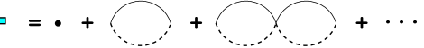
FIG. 1.: Bubble graphs that contribute to the composite particle propagator. Solid line represents the spin-1/2 quark and dashed line represents the spin-0 boson.

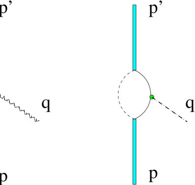
FIG. 2.: Photon-quark and pion-quark insertions in the composite particle propagator.

FIG. 3.: Electromagnetic and pion form factors for composite particle.

FIG. 4.: Dependence of form factor F${}_{1}^{++}$, including propagator factor as discussed in text, on off-mass-shell variable p², where p²/M² = 1.2 (dot line), 1.1 (dashed line), 1.0 (solid line), 0.9 (dot-dash line and 0.8 (long-dash line).

FIG. 5.: Dependence of the ratio $F_{1}^{+-}(Q^{2},M^{2},p^{2})/F_{1}^{++}(Q^{2})$ on off-mass-shell variable p², where p²/M² = 1.2 (dot line), 1.1 (dashed line), 1.0 (solid line), 0.9 (dot-dash line and 0.8 (long-dash line). Propagator factor is included as discussed in text.

FIG. 6.: Dependence of ratio $F_{2}^{+-}(Q^{2},M^{2},p^{2})/F_{2}^{++}(Q^{2})$ on off-mass-shell variable p², where p²/M² = 1.2 (dot line), 1.1 (dashed line), 1.0 (solid line), 0.9 (dot-dash line and 0.8 (long-dash line). Propagator factor is included as discussed in text.

FIG. 7.: Dependence of form factor $F_{5}^{+-}(Q^{2},M^{2},p^{2})/F_{5}^{++}(Q^{2})$ on off-mass-shell variable p², where p²/M² = 1.2 (dot line), 1.1 (dashed line), 1.0 (solid line), 0.9 (dot-dash line and 0.8 (long-dash line). Propagator factor is included as discussed in text.

FIG. 8.: Pseudovector fraction of pion-nucleon coupling.

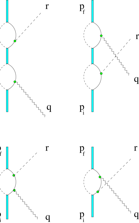
FIG. 9.: Photopion amplitudes. Top: direct and crossed Born graphs. Bottom: direct and crossed contact-like graphs.

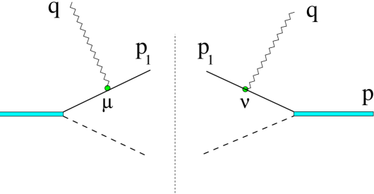
FIG. 10.: Impulse approximation for deep inelastic scattering.

FIG. 11.: Structure function for inelastic scattering. Q = 1.5 GeV/c (dot line), Q= 2.5 GeV/c (dash line), Q = $\infty$ (solid line).

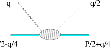
FIG. 12.: Quasifree kinematics for photopion amplitude in meson-exchange current. The pion (dashed line) is absorbed by a second nucleon, not shown, such that the each nucleon absorbs half the photon momentum.

FIG. 13.: Born amplitude (solid line) is compared with product of dipole form factors and propagator (dotted line). Contact-like contribution (long dash line) is compared with estimate based on product of dipole form factor and factor S(Q) = $\kappa^{2}/(Q^{2}+\kappa^{2})$, with $\kappa$ = 0.2 GeV², (dotted line).

FIG. 14.: Isospin-nonflip a amplitude: full amplitude (solid line), elementary amplitude based on pseudoscalar pion coupling (dash line), nonrelativistic amplitude (dot line) and Born amplitude of composite model (long dash line).

FIG. 15.: Contact-like contribution of composite model (solid line), excited states and Z-graph part of Born amplitude for composite model (long dash line), sum of contact-like, excited states and Z-graph parts (dot dash line) and Z-graph part of pseudoscalar elementary amplitude (dash line).

FIG. 16.: Isospin-nonflip a amplitude: full amplitude (solid line), elementary amplitude based on pseudovector pion coupling (dash line), nonrelativistic amplitude (dot line) and Born amplitude of composite model (long dash line).

FIG. 17.: Contact-like contribution of composite model (solid line), excited states and Z-graph part of Born amplitude for composite model (long dash line), sum of contact-like, excited states and Z-graph parts (dot dash line) and difference between elementary amplitude based on pseudovector pion coupling and nonrelativistic amplitude (dash line).

FIG. 18.: Isospin-flip b amplitude: full amplitude (solid line), elementary amplitude based on pseudoscalar pion coupling (dash line), nonrelativistic amplitude (dot line) and Born amplitude of composite model (long dash line).

FIG. 19.: Isospin-flip c amplitude: full amplitude (solid line), elementary amplitude based on pseudoscalar pion coupling (dash line), nonrelativistic amplitude (dot line) and Born amplitude of composite model (long dash line).

REFERENCES

• [1] B. S. Pudliner, V. R. Pandharipande, J. Carlson, S. C. Pieper and R. B. Wiringa, Phys. Rev. C56, 1720 (1997).
• [2] J. Carlson and R. Schiavilla, Rev. Mod. Phys., 70, 743 (1998).
• [3] J. Fleischer and J. A. Tjon, Phys. Rev. D 15, 2537 (1977).
• [4] M. M. Nagels, T. A. Rijken and J. J. de Swart, Phys. Rev. D 17, 768 (1978).
• [5] R. Machleidt, K. Holinde and Ch. Elster, Phys. Rept. 149, 1 (1987).
• [6] J. D. Bjorken, Phys. Rev. 179, 1547 (1969).
• [7] R. P. Feynman, Photon Hadron Interactions (Benjamin, New York, 1972).
• [8] C. Bochna, et al., Phys. Rev. Lett. 81, 4576 (1998).
• [9] N. Isgur and C. Llewellyn Smith, Phys. Rev. Lett. 52, 1080 (1984); Nucl. Phys. B317, 526 (1989).
• [10] F. E. Low, Phys. Rev. 110 (1958) 974.
• [11] S. J. Wallace, F. Gross and J. A. Tjon, Phys. Rev. Lett. 74, 228 (1995); Phys. Rev. C53, 860 (1996).
• [12] D. R. Phillips, M. C. Birse and S. J. Wallace, Phys. Rev. C55, 1937 (1997).
• [13] X. Ji, Phys. Rev. D55, 7114 (1997).
• [14] A. V. Radyushkin, Phys. Lett. B380, 417 (1996).
• [15] W. Pauli and F. Villars, Rev. Mod. Phys. 21, 4334 (1949).
• [16] J. C. Ward, Phys. Rev. 78, 182 (1950).
• [17] Y. Takahashi, Nuovo Cimento 6, 371 (1957).
• [18] P. C. Tiemeijer and J. A. Tjon, Phys. Rev. C42, 599 (1990).
• [19] H. W. L. Naus and J. H. Koch, Phys. Rev. C39, 1907 (1989).
• [20] F.-F. Mathiot, Phys. Rept. 173, 63 (1989).
• [21] D. O. Riska, Phys. Rept. 181, 207 (1989).
• [22] G. West, Phys. Rept. 18, 263 (1975).
• [23] R. G. Roberts, The Structure of the Proton (1990).
• [24] C. Callan and D. Gross, Phys. Rev. Lett. 22, 156 (1969).
• [25] Z. Batiz and F. Gross, Phys. Rev. C 58, 2963 (1998).
• [26] H. Mineo, W. Bentz and K. Yazaki, Phys. Rev. C 60, 06520 (1999).
• [27] M. Veltman, private communication; see also G. Passarino and M. Veltman, Nucl. Phys. B160, 151 (1979).
Refer to caption