Dynamics of Hot Bulk QCD Matter: from the Quark-Gluon Plasma to Hadronic Freeze-Out

Abstract

We introduce a combined macroscopic/microscopic transport approach employing relativistic hydrodynamics for the early, dense, deconfined stage of the reaction and a microscopic non-equilibrium model for the later hadronic stage where the equilibrium assumptions are not valid anymore. Within this approach we study the dynamics of hot, bulk QCD matter, which is expected to be created in ultra-relativistic heavy ion collisions at the SPS, the RHIC and the LHC. Our approach is capable of self-consistently calculating the freeze-out of the hadronic system, while accounting for the collective flow on the hadronization hypersurface generated by the QGP expansion. In particular, we perform a detailed analysis of the reaction dynamics, hadronic freeze-out, and transverse flow.

I Introduction

A major goal of colliding heavy-ions at relativistic energies is to heat up a tiny region of space-time to temperatures as high as are thought to have occured during the early evolution of the universe, a few microseconds after the big bang [1]. In ultra-relativistic heavy-ion collisions the four-volume of hot and dense matter, with temperatures above $\sim 150$ MeV, is on the order of $\sim(10$ fm$)^{4}$. The state of strongly interacting matter at such high temperatures (or density of quanta) is usually called quark-gluon plasma (QGP) [2]. For a discussion of the properties and potential signatures of such a super-dense state see [2, 3].

A particularly interesting aspect of producing such a hot and dense space-time region is that QCD, the fundamental theory of strong interactions, is expected to exhibit a transition to a new thermodynamical phase at a critical temperature $T_{C}\sim 100-300$ MeV. This phase transition has been observed in numerical studies of the thermodynamics of QCD at vanishing net baryon charge on lattices [4]. It is the only phase transition of a fundamental theory that is accessible to experiments under controlled laboratory conditions.

In this paper we shall investigate the dynamics of relativistic heavy ion collisions within a novel transport approach combining a macroscopic and a microscopic model. We shall focus here on collision systems currently under investigation at the CERN Super-Proton-Synchrotron (SPS), the Relativistic Heavy Ion Collider (RHIC) at BNL and the future Large Hadron Collider (LHC) at CERN.

We shall work in natural units $\hbar=c=k=1$ throughout the paper.

II General Aspects of Matching Fluid Dynamics to Microscopic Transport

In this section we discuss general aspects and assumptions of our model for the space-time evolution of high-energy heavy-ion reactions. In particular, we introduce fluid dynamics for the early, hot stage, and the matching to microscopic transport for the later, more dilute stages of the reaction. Within this section, quantities without subscript refer to the fluid, while properties of the microscopic transport theory carry the subscript $micro$.

A Transport Equation for Incoherent Quanta / Particles

The most basic assumption of our model for the evolution of high-energy heavy-ion reactions is that at the initial time $t=t_{i}$ the highly excited space-time domain produced in the impact can be viewed as being populated by incoherent quanta on the mass-shell. Thus, the system can be described by a distribution function $f_{i}(x^{\mu},p^{\nu})$, where $x^{0}=t_{i}$, $p^{0}=\sqrt{\vec{p}^{2}+m_{i}^{2}}$, and $i$ labels different species of quanta. We will not discuss here how such a state of high entropy density could possibly be reached. That discussion is out of the scope of the present manuscript. Our work addresses the subsequent evolution of that initial state up to the so-called freeze-out of strong interactions in the system.

The semi-classical evolution of the distribution function in the forward light-cone is described by means of a so-called transport equation, e.g. the Boltzmann equation [5]

$$p\cdot\partial f_{i}(x^{\mu},p^{\nu})={\cal C}_{i}\quad.$$ (1)

${\cal C}_{i}$ is the collision kernel, describing gain or loss of quanta (particles) of species $i$ in the phase-space cell around $(x^{\mu},p^{\nu})$ due to collisions. Note that we have dropped possible classical background fields in eq. (1).

B Moments of the Transport Equation: Hydrodynamics for the hottest stage

For the problem at hand, however, the usefulness of eq. (1) is rather limited. A major difficulty is that to obtain an analytical or numerical solution, in most cases one has to introduce an expansion of the collision kernel in terms of the number of incoming particles per “elementary” collision [5] (In most practical applications that expansion is even truncated at the level of binary collisions, $2\rightarrow n$). Obviously, the expansion is ill-defined at very high densities. A second major problem is to describe the hadronization process, i.e. the dynamical conversion of quarks and gluons into hadrons, on the microscopic level. Several interesting approaches to describe the hadronization of a plasma of quarks and gluons microscopically have been proposed in the literature, cf. e.g. [6] and references therein. However, due to the very complicated nature of this process, many of those models have to involve some kind of ad-hoc prescriptions, which have quite significant impact on the results. A first-order QCD phase transition, as assumed in the following, is particularly difficult to model microscopically.

At present we are not able to solve these problems in a fully satisfactory way. We can, however, circumvent them to some extent if we are mainly interested in the bulk dynamics of a hot QCD system. In this case we can employ relativistic ideal hydrodynamics [7] for the very dense stage of the reaction up to hadronization.

Let us thus assume that it is feasible to employ the continuum limit. The first two moments of eq. (1) yield the continuity equations for the conserved currents and for energy and momentum [5],

$$\partial\cdot N_{i}=0\quad,\quad\partial\cdot\Theta=0\quad.$$ (2)

In the following, we will explicitly consider only one conserved current, namely the (net) baryon current. All other currents, as e.g. strangeness, charm, electric charge etc., will be assumed to vanish identically (due to local charge neutrality and an ideal fluid) such that the corresponding continuity equations are trivially satisfied.

Ideal fluid dynamics goes even further and assumes that the momentum-space distributions in the local rest frame are given by either Fermi-Dirac or Bose-Einstein distribution functions, respectively. Dissipation and heat conduction which arise from higher moments are neglected. Since we restrict fluid-dynamics to the high-temperature and high-density stage, this approximation is at least logically consistent. In future work, it will be important though to check its quantitative accuracy.

The density of secondary partons in the central region of high-energy nuclear collisions is very high. According to present knowledge, it is likely that the central region evolves from a stage of pre-equilibrium towards a QGP in local thermal equilibrium [8, 9, 10, 11], despite the large expansion rate. On the other hand, the very same calculations do not seem to support rapid chemical equilibration (in particular of the quarks), cf. also [12, 13, 14]. However, in most publications interactions among the secondary partons (and in particular particle production via inelastic processes) were treated perturbatively. Since the running coupling in a thermal plasma with $T\leq 1$ GeV is not very small, one can not exclude sizeable contributions from processes involving higher powers of $\alpha_{s}$ [10]. Moreover, in addition to the semi-hard partons there might exist a coherent color field in the central region (between the receding nuclear “pancakes”) which produces additional quark-antiquark pairs in its decay [15]. In any case, we will not argue in favor nor against rapid $q\overline{q}$ production and chemical equilibration but simply assume that the quark densities at the initial time of the hydrodynamical expansion are close to their chemical equilibrium values. At least for Pb+Pb at CERN-SPS energy, where experimental data already exists, this is basically the only way for our model to account for the fact that measured hadron multiplicity ratios are close to their chemical equilibrium values [16]. Since the expansion rate after hadronization is too large for “chemical cooking” (and in particular for strangeness equilibration), as will be discussed in section IV D, it would be virtually impossible to achieve approximate chemical equilibrium during the later hadronic stages if starting from a QGP far off chemical equilibrium, cf. also [17].

The general picture as described above is summarized in the space-time diagram depicted in Fig. 1. We assume that ideal fluid dynamics is a reasonable approximation between the “initial” time $t_{i}$ and the hadronization hypersurface. After that, we will switch to a microscopic description employing the binary collision approximation for the collision kernel. In particular, we will employ the Ultrarelativistic Quantum Molecular Dynamics (UrQMD) transport model, see below.

C Microscopic Transport from Hadronization to Freeze-Out

One may ask why it is not sufficient to rely on hydrodynamics up to some rather late stage of the reaction, after which one postulates that all particle momenta are “frozen” and thus are equal to those measured in the detector at $t_{f}\rightarrow\infty$. That approach has been applied to nuclear collisions by many authors, for recent work cf. e.g. [18, 19, 20, 21], and leads to reasonable results for the single-particle spectra of the most abundant hadron species $\pi$, $K$, $p$, $\Lambda$. However, the following limitations arise:

First, the evolution must clearly be non-ideal in the late stages of the reaction [22], as the system approaches “freeze-out”. This can manifest in decoupling of various components of the fluid (e.g. pions and nucleons), i.e. each component develops an individual collective velocity [23]. Another aspect is that the $-p{\rm d}V$ expansion work performed by the fluid can be partly compensated by entropy production ($+T{\rm d}S$) such that the expansion may even become isoergic, ${\rm d}E=0$, instead of isentropic, ${\rm d}S=0$ [24].

Moreover, since each hadron is propagated individually, and its interactions with other hadrons are described on the basis of elementary processes, microscopic transport models offer the opportunity to calculate the freeze-out conditions instead of just putting them in by hand as is done in the purely fluid-dynamical approaches [18, 19, 20, 21]. There one assumes that freeze-out occurs whenever some criterion is fulfilled, e.g. when the temperature drops below some “guessed” value. In contrast, the non-truncated transport eq. (1) can describe self-consistently the freeze-out of the system: no decoupling hypersurface is imposed by hand, but rather is determined by an interplay between the (local) expansion scalar $\partial\cdot u$ [1, 25, 26, 27] (where $u$ is the four-velocity of the local rest-frame), the relevant elementary cross sections and decay rates, and the equation of state (EoS), which actually changes dynamically as more and more hadron species decouple. This is obviously a key point for being able to study and predict the dependence of the final state on collision energy (i.e. on the initial entropy or energy density), system size etc., instead of just fitting it by an appropriate choice of a freeze-out hypersurface. Note e.g. that the nucleons emerging from the QCD hadronization phase transition in the early universe were able to maintain chemical equilibrium down to temperatures of about $\sim 50$ MeV [1]. In heavy-ion collisions at CERN-SPS energies, however, one finds chemical freeze-out temperatures on the order of $140-160$ MeV [16]. The origin of this difference lies in the much smaller expansion rate (Hubble constant) of the early universe as compared to a high-energy heavy ion collision [27], and can only be explained within kinetic theory but not within pure hydrodynamics.

Another complication arises from the fact that close to the freeze-out hypersurface the freeze-out process feeds back on the evolution of the fluid [28, 29, 30]. This will in general deform the freeze-out hypersurface, say an isotherm of given temperature $T_{fo}$. It will differ from that found a posteriori from the solution of eqs. (2) in the whole forward light-cone. Furthermore, the idealization that the transition from ideal flow to free-streaming occurs on a sharp hypersurface, i.e. a three-volume in space-time, is rather crude. One instead expects a smooth transition as the temperature (and the density of particles) decreases, cf. e.g. the discussion in [31]. This is supported by studies of the hadron kinetics close to freeze-out with realistic cross-sections [32, 33], cf. also section IV C.

Finally, it is likely that the freeze-out is not universal for all hadron species, simply because their transport cross-sections are very different. One can therefore hardly assume that all hadron species decouple on the same hypersurface [26, 32, 33, 34]. The clearest example for this is the transverse momentum distribution of $\Omega$ baryons obtained by the WA97 collaboration [35] for Pb+Pb collisions at CERN-SPS energy, $\sqrt{s}=17A$ GeV. Unlike is the case for pions, nucleons, anti-nucleons, and lambdas, the $p_{T}$ distribution of omegas as calculated within hydrodynamics with freeze-out on the $T=T_{fo}=130$ MeV hypersurface [21] is much stiffer than the experimental finding. Indeed, more detailed kinetic treatments which explicitly account for the small transport cross-section of $\Omega$ baryons in a meson-rich hadron gas, emerging either from fragmentation of longitudinally stretched color-strings [36] or an incoherent hot plasma of quarks and gluons [37], show that these multiple-strange particles freeze out earlier and pick up less collective transverse flow than pions and nucleons, for example.

D Transition from Fluid Dynamics to Microscopic Transport

A few remarks on the transition from hydrodynamics to microscopic transport are in order here. In general, one should introduce source terms $-\partial\cdot N_{micro}$ and $-\partial\cdot\Theta_{micro}$ on the right-hand-sides of eqs. (2), where

$$N_{micro}^{\mu}(x) = \sum_{i}\int\frac{{\rm d}^{3}k}{k^{0}_{i}}k^{\mu}f_{i,{\rm micro}}(x,k)\quad,$$ (3)

$$\Theta_{micro}^{\mu\nu}(x) = \sum_{i}\int\frac{{\rm d}^{3}k}{k^{0}_{i}}k^{\mu}k^{\nu}f_{i,{\rm micro}}(x,k)$$ (4)

denote the net baryon current and the energy-momentum tensor of the microscopic transport model, respectively. Accordingly, external sources of particles have to be introduced in the transport equation, which model the net-baryon charge and energy-momentum transfer from the fluid. This way a self-consistent solution in the whole forward light-cone, starting from the initial hypersurface $t=t_{i}$ could be obtained.

However, if a space-time region bounded by a hypersurface $\sigma^{\mu}_{H}$ exists where fluid-dynamics is an adequate approximation, one can choose an arbitrary hypersurface $\sigma^{\mu}_{switch}$ within this region where to switch from eqs. (2) to (1). One can then simply assume $N_{micro}\equiv 0$ and $\Theta_{micro}\equiv 0$ in the interior, and $N\equiv 0$, $\Theta\equiv 0$ in the exterior. On that hypersurface, one sets $N_{micro}\equiv N$, $\Theta_{micro}\equiv\Theta$. This is because hydrodynamics is a limiting case of eq. (1), and this more general transport equation will automatically recover the fluid-dynamical solution in the space-time region between $\sigma^{\mu}_{switch}$ and $\sigma^{\mu}_{H}$.

For the particular model discussed here, $\sigma^{\mu}_{switch}$ can not precede the hadronization hypersurface since our microscopic transport model deals with color-singlet states, only. Also, it employs the binary collision approximation of the kernel, which becomes less justified in the hot and dense stage preceding hadronization.

Furthermore, as will be discussed in more detail below, in high-energy heavy-ion collisions it turns out that the boundary of validity of (ideal) fluid dynamics, $\sigma^{\mu}_{H}$, can not extend far into the post-hadronization stage (the less the higher the collision energy). Thus, we conclude that the hadronization hypersurface is the most natural choice for the switch from eqs. (2) to (1).

The phase-space distribution of particles of species $i$ on $\sigma^{\mu}_{switch}$ is then given by [38]

$$E_{i}\frac{{\rm d}N_{i}}{{\rm d}^{3}p}=\int{\rm d}\sigma\cdot p\,\,f(p\cdot u),$$ (5)

where $u^{\mu}$ is the four-velocity of the local rest-frame. An explicit expression for the geometry suitable for high-energy collisions will be given below. For time-orthogonal hypersurfaces as depicted in Fig. 1 one has

$${\rm d}\sigma_{\mu}\Big{|}_{t={\rm const.}}=({\rm d}^{3}x,\vec{0})\quad,$$ (6)

the left-hand-side of eq. (5) being simply $E_{i}f_{i,micro}$.

It is clear that by construction the microscopic transport starts from a state of local equilibrium on $\sigma^{\mu}_{switch}$, the hypersurface where the switch is performed. The local energy density, net baryon density, and collective expansion velocity are those obtained from the hydrodynamical solution. Thus, the conserved currents and the energy-momentum tensor of the microscopic transport theory assume the form appropriate for ideal fluids [7],

$$N_{micro}^{\mu} = \rho u^{\mu}\quad,$$ (7)

$$\Theta_{micro}^{\mu\nu} = \left(\epsilon+p_{micro}\right)u^{\mu}u^{\nu}-p_{micro}g^{\mu\nu}\quad.$$ (8)

Now, in order that $\Theta_{micro}=\Theta$ on $\sigma^{\mu}_{switch}$, the pressure at given energy and baryon density must equal that of the fluid-dynamical model, i.e., the equations of state in local thermodynamical equilibrium must be the same. In general this requirement is non-trivial. For ideal gases, however, it can be obeyed by simply including the same states $i$ in the microscopic transport  (1) as in the grand partition function which is used to calculate the equation of state employed in hydrodynamics. We shall discuss this point in more detail when presenting our specific equation of state below.

We finally briefly discuss one last aspect of the switch from fluid dynamics to microscopic transport on some hypersurface $\sigma^{\mu}_{switch}$. As already mentioned above, this hypersurface is assumed to be within the region of validity of ideal hydrodynamics, and should be identified with the hadronization hypersurface. However, the latter will in general also exhibit time-like parts (points where the normal vector on $\sigma^{\mu}_{switch}$ is space-like). A schematic example is given in Fig. 2. The initial condition of the microscopic transport on $\sigma^{\mu}_{switch}$ can now not be chosen arbitrarily. This is clear from the fact that the points 1 and 2, for example, are causally connected. The simplest way to prevent violation of the evolution equations is to specify initial conditions on a purely space-like hypersurface (e.g. $t=t_{i}$) and to employ the dynamical equations, in our case the continuity equations (2), to calculate $\Theta$ and $N$ on $\sigma^{\mu}_{switch}$. This way the states of the system at 1 and at 2 are consistent.

However, one problem with switching on a hypersurface with time-like parts remains. As discussed above, eq. (5) conserves energy-momentum and (net) baryon charge. For this to hold, it actually does not count the flow of the currents from the inside to the outside of $\sigma^{\mu}_{switch}$ but, actually, the net flow. That is, the difference of outflowing and inflowing charge, momentum etc. The inflow is due to those parts of the thermal distribution function $f(x,p)$ which move into the opposite direction than the fluid. Due to the exponential tails of $f$ such particles clearly always exist, but their number decreases strongly if the collective flow is strong. In this case the locally isotropic momentum-space distribution is strongly boosted.

Thus, the in-current is obtained under the assumption that within an infinitesimal region on both sides of the hypersurface there is hydrodynamic flow and local thermodynamical equilibrium. For this reason, $\sigma^{\mu}_{switch}$ must be entirely within the region of validity of fluid dynamics, $\sigma^{\mu}_{H}$. Again, in this case eq. (5) gives the net flow of all the currents from the fluid-region to the region where we apply the microscopic transport.

The problem is, however, that in some part of momentum and coordinate space the left-hand-side of eq. (5) can be negative. This means that the ingoing flow exceeds the outgoing flow. These “negative contributions” were already discussed by several authors [28, 29, 39]. Since we will interpret ${\rm d}^{3}p\,{\rm d}\sigma\cdot pf(p\cdot u)/E$ as a probability distribution we have to require positive definiteness. This can either be achieved by multiplying with a cut-off function $\Theta({\rm d}\sigma\cdot p)$, which leads to a slight violation of the conservation laws; or by integration over sufficiently large bins in momentum and coordinate-space, and random redistribution of the particles within the bins, which smears out the distribution over momentum and coordinate space.

A rigorous solution of this problem requires to introduce the above-mentioned source-terms in the fluid-dynamical evolution equations as well as in the microscopic transport equation. However, for the cases studied here the negative contributions were not relevant. The main reason is that the collective flow velocity on the time-like parts of the hypersurface is close to one, such that net flow of particles from the microscopic transport to hydrodynamics does not occur. For non-relativistic flow on $\sigma^{\mu}_{switch}$, however, the negative contributions would be more serious.

III Specific Model for High-Energy Heavy-Ion Collisions

In the present paper we shall use hydrodynamics to model a first order phase transition from a QGP to a hadronic fluid, and combine it with a microscopic transport calculation for the later, purely hadronic stages of the reaction.

In the following sections we describe the particular hydrodynamical and transport models employed here, cf. also [21] and [40].

A Scaling Hydrodynamics

As already mentioned above, hydrodynamics for hadronic collisions is defined by (local) energy-momentum and net baryon charge conservation,

$$\partial\cdot\Theta=0\quad,\quad\partial\cdot N_{B}=0\quad.$$ (9)

$\Theta^{\mu\nu}$ denotes the energy-momentum tensor, and $N_{B}^{\mu}$ the current of net baryon charge.

For ideal fluids, the energy-momentum tensor and the net baryon current assume the simple form [7]

$$\Theta^{\mu\nu}=\left(\epsilon+p\right)u^{\mu}u^{\nu}-pg^{\mu\nu}\quad,\quad N_{B}^{\mu}=\rho_{B}u^{\mu}\quad,$$ (10)

where $\epsilon$, $p$, $\rho_{B}$ are energy density, pressure, and net baryon density in the local rest frame of the fluid, which is defined by $N_{B}^{\mu}=(\rho_{B},\vec{0})$. Let us, in the following, work in the metric $g^{\mu\nu}={\rm diag}(+,-,-,-)$. $u^{\mu}=\gamma(1,\vec{v})$ is the four-velocity of the fluid ($\vec{v}$ is the three-velocity and $\gamma=(1-\vec{v}^{2})^{-1/2}$ the Lorentz factor). The system of partial differential equations (9) is closed by choosing an equation of state (EoS) in the form $p=p(\epsilon,\rho_{B})$, cf. below.

For simplicity, we assume a cylindrically symmetric transverse expansion with a longitudinal scaling flow profile, $v_{z}=z/t$ [41]. At $z=0$, equations (9) reduce to

$$\partial_{t}E+\partial_{T}\left[\left(E+p\right)v_{T}\right] = -\left(\frac{v_{T}}{r_{T}}+\frac{1}{t}\right)\left(E+p\right)\quad,$$ (11)

$$\partial_{t}M+\partial_{T}\left(Mv_{T}+p\right) = -\left(\frac{v_{T}}{r_{T}}+\frac{1}{t}\right)M\quad,$$ (12)

$$\partial_{t}R+\partial_{T}\left(Rv_{T}\right) = -\left(\frac{v_{T}}{r_{T}}+\frac{1}{t}\right)R\quad,$$ (13)

where we defined $E\equiv\Theta^{00}$, $M\equiv\Theta^{0T}$, and $R\equiv N_{B}^{0}$. In the above expressions, the index $T$ refers to the transverse component of the corresponding quantity.

The set of equations (11) describes the evolution in the $z=0$ plane. Due to the assumption of longitudinal scaling, the solution at any other $z\neq 0$ can be simply obtained by a Lorentz boost. The above equations also imply

$$\left.\frac{\partial p}{\partial\eta}\right|_{\tau,r_{T}}=0\quad,$$ (14)

where $\eta\equiv{\rm Artanh}~{}v_{z}$ and $\tau\equiv\sqrt{t^{2}-z^{2}}$. This means that on $\tau={\rm const.}$ hypersurfaces pressure gradients in rapidity direction vanish, and there is no flow between adjacent infinitesimal rapidity slices. However, only for net baryon free matter, $\rho_{B}\equiv 0$, does this automatically also mean that the temperature $T$ is independent of the longitudinal fluid rapidity $\eta$. In the case $\rho_{B}\neq 0$ equation (14) only demands

$$\left.s\frac{\partial T}{\partial\eta}\right|_{\tau}+\left.\rho_{B}\frac{\partial\mu_{B}}{\partial\eta}\right|_{\tau}=0\quad.$$ (15)

$s$ and $\mu_{B}$ denote entropy density and baryon-chemical potential, respectively. If other charges like strangeness or electric charge are locally non-vanishing, additional terms appear. Equation (15) does not imply that the rapidity distribution of produced particles is flat (i.e. independent of rapidity) or that the rapidity distributions of various species of hadrons, e.g. pions, kaons, and nucleons, are similar. Any rapidity-dependent $T$ and $\mu_{B}$ that satisfy eq. (15) are in agreement with energy-momentum and net baryon number conservation, as well as with longitudinal scaling flow $v_{z}=z/t$ [42]. Note also that non-trivial solutions of eq. (15) in general also yield ${\partial}\mu_{S}/{\partial}\eta\neq 0$ on the hadronization hypersurface (i.e. a rapidity-dependent strangeness-chemical potential), even if the strangeness-density $\rho_{S}=0$ everywhere in the forward light-cone. In this paper, however, we do not explore the rapidity dependence of the particle spectra, and thus simply assume that $T$ and $\mu_{B}$ are independent of $\eta$.

The fluid-dynamical evolution equations can be solved numerically on a discretized space-time grid, cf. e.g. [43, 44].

B Equation of State

To close the system of coupled equations of hydrodynamics, an equation of state (EoS) has to be specified. From eq. (10) it follows that for an ideal gas the pressure $p$ is given by

$$p=q\cdot\left(q\cdot\Theta\right)\quad,$$ (16)

where $q^{\mu}$ is orthogonal to $u^{\mu}$ and normalized to $q\cdot q=-1$. In particular, in the local rest-frame $u^{\mu}=(1,\vec{0})$, we can choose $q^{\mu}\propto(0,1,0,0)+(0,0,1,0)+(0,0,0,1)$. Then, from the definition of the energy-momentum tensor from kinetic theory, eq. (4), we obtain

$$p(T,\mu_{B},\mu_{S})=\sum_{i}\int\frac{{\rm d}^{3}k}{k^{0}_{i}}\frac{\vec{k}^{2}}{3}f_{i}(k;T,\mu_{B},\mu_{S})\quad.$$ (17)

The sum over $i$ extends over the various particle species. The grand canonical potential is given by $\Omega=-pV$, where $V\equiv\int{\rm d}\sigma\cdot u$ denotes the three-volume of the given hypersurface of homogeneity. All other quantities can be obtained via standard thermodynamical relationships. E.g., the densities of entropy, net baryon charge, and energy are given by

$$s(T,\mu_{B},\mu_{S}) = \frac{\partial p(T,\mu_{B},\mu_{S})}{\partial T}\quad,$$ (18)

$$\rho_{B}(T,\mu_{B},\mu_{S}) = \frac{\partial p(T,\mu_{B},\mu_{S})}{\partial\mu_{B}}\quad,$$ (19)

$$\rho_{S}(T,\mu_{B},\mu_{S}) = \frac{\partial p(T,\mu_{B},\mu_{S})}{\partial\mu_{S}}\stackrel{{\scriptstyle!}}{{=}}0\quad,$$ (20)

$$\epsilon(T,\mu_{B},\mu_{S}) = Ts-p+\mu_{B}\rho_{B}\quad.$$ (21)

From $p(T,\mu_{B},\mu_{S})$, $\rho_{B}(T,\mu_{B},\mu_{S})$ and $\epsilon(T,\mu_{B},\mu_{S})$ one can construct the function $p(\epsilon,\rho_{B})$ which is needed to close the system of continuity equations (9).

So far, we discussed an ideal gas, only. However, lattice QCD predicts a phase transition from ordinary nuclear matter to a so-called quark-gluon plasma (QGP) at a critical temperature of $T_{C}=140-160$ MeV [4] (for $\rho_{B}=0$). We will employ a very simple and intuitive, though not very well justified description of this phase transition. We model the high-temperature phase as an ideal gas of $u$, $d$, $s$ quarks (with masses $m_{u}=m_{d}=0$, $m_{s}=150$ MeV), and gluons, employing the well-known MIT bag model EoS [2, 45]. In this model the non-perturbative interactions of the “deconfined bag” of quarks and gluons with the true vacuum are parameterized by a bag constant $B$. To make this state thermodynamically unfavorable at low temperatures, the bag contribution to the pressure must be negative. Thus, when computing the pressure of the QGP phase we subtract $B$ from the right-hand-side of eq. (17). Accordingly, the energy density receives a positive contribution, cf. (21), while $s$ and $\rho_{B}$ remain unchanged. This additional “bag term” can also be understood as an additional contribution $+Bg^{\mu\nu}$ due to the non-perturbative interactions to the energy-momentum tensor of the QGP-fluid.

In the low-temperature region we assume an ideal hadron gas that includes the well-established (strange and non-strange) hadrons up to masses of $\sim 2$ GeV. They are listed in Tab. I and II. Although heavy states are rare in thermodynamical equilibrium, they have a larger entropy per particle than light states, and therefore have considerable impact on the evolution. In particular, hadronization is significantly faster as compared to the case where the hadron gas consists of light mesons only (see the discussion in [18, 19, 21, 30, 46]).

The actual model used for the hadronic stage of the reaction (UrQMD, see section III D) additionally assumes a continuum of color-singlet states called “strings” above the $m\simeq 2$ GeV threshold to model $2\rightarrow n$ processes and inelastic processes at high CM-energy. For example, the annihilation of an $\overline{p}$ on an $\Omega$ is described as excitation of two strings with the same quantum numbers as the incoming hadrons, respectively, which are subsequently mapped on known hadronic states according to a fragmentation scheme. Since we shall be interested in the dynamics of the $\Omega$-baryons emerging from the hadronization of the QGP, it is unavoidable to treat string-formation. The fact that string degrees of freedom are not taken into account in the EoS (17) does not represent a problem in our case because we focus on rapidly expanding systems where those degrees of freedom can not equilibrate [47].

The phase coexistence region is constructed employing Gibbs’ conditions of phase equilibrium. The bag parameter of $B=380$ MeV/fm³ is chosen to yield the critical temperature $T_{C}\approx 160$ MeV at $\rho_{B}=0$. By construction the EoS exhibits a first order phase transition, as is also expected in QCD for the quark-hadron phase transition in the case of three light quark flavors [48].

The most striking aspect of a first-order phase transition with respect to the dynamical evolution is that the pressure is almost constant within the phase coexistence region (in fact, in a fluid where all conserved currents vanish identically $p={\rm const.}$ within the mixed phase). Thus, the isentropic speed of sound,

$$c_{S}^{2}=\frac{{\partial}p}{{\partial}\epsilon}\Big{|}_{s/\rho_{B}}\quad,$$ (22)

is very small. This quantity characterizes the pressure gradient caused by a given energy density gradient along an isentrope, i.e. at constant entropy density per net baryon density (recall that all continuous solutions of the relativistic ideal-fluid dynamical equations conserve the entropy). A very small $c_{S}$ means that (isentropic) expansion is inhibited because the fluid does not “respond” to energy density gradients. In heavy-ion collisions this reflects in a particularly “soft” expansion if the mixed phase occupies the largest space-time volume of all three phases [21, 44, 49, 50, 51]. For recent discussions of the consequences of this effect in cosmology (primordial black hole formation, evolution of density perturbations through the QCD phase transition) see e.g. [52].

However, a nearly vanishing isentropic velocity of sound does only occur if the net baryon density is not very large, as e.g. in the cosmological QCD phase transition or in the central region of high-energy collisions studied here. In heavy-ion collisions at much lower energies, where the net baryon density in the central region is rather large, $c_{S}$ is not very small. Despite the first-order phase transition, the isentropic expansion of baryon-dense fluids is not inhibited [53].

One should also be aware of the fact that by constructing the phase coexistence region with Gibbs’ conditions we implicitly assume a “well-mixed” phase, i.e. that the transition from the QGP to the hadronic stage proceeds in equilibrium. This is the common approach widely employed in the literature [18, 19, 20, 21, 26, 30, 33, 37, 43, 44, 46, 49, 50, 51, 53, 54, 55], and so far it is not in contradiction to existing data. It is based on the picture that the first-order phase transition proceeds via nucleation of hadronic bubbles in the expanding QGP [56], and that the bubble nucleation and growth is fast as compared to the expansion rate such that the two phases are approximately in pressure equilibrium. However, this scenario is less likely to apply to high-energy heavy-ion collisions than to the cosmological QCD phase transition, because in the former case the expansion rate is many order of magnitude larger [27]. In particular, it has been speculated recently that the time-scale for supercooling down to the spinodal instability is comparable to that for homogeneous bubble nucleation [57]. Thus, it may well be that the phase transition proceeds via spinodal decomposition rather than bubble nucleation. In that case, the “soft” mixed phase with $c_{s}^{2}\approx 0$ would be absent and shorter reaction times may be expected. In any case, we postpone a detailed dynamical study of the latter scenario to a future publication, and shall restrict ourselves here to the more conservative picture assuming an adiabatic phase transition.

Finally, we have to specify the initial conditions:

• For collisions at SPS energy we assume that hydrodynamic flow sets in on the hyperbola $\tau_{i}=1$ fm/c. This is a value conventionally assumed in the literature, cf. e.g. [41]. We further employ a (net) baryon rapidity density (at mid-rapidity) of $dN_{B}/dy=80$, as obtained by the NA49-collaboration for central Pb+Pb reactions [58]. The average specific entropy in these collisions is $\overline{s}/\overline{\rho}_{B}=45\pm 5$ (the bar indicates averaging over the transverse plane). That entropy per net baryon fits most measured hadron multiplicity ratios within $\pm 20\%$ [16]. The corresponding initial energy and net baryon densities ($\overline{\epsilon}_{i}=6.1$ GeV/fm³, $\overline{\rho}_{i}=4.5\rho_{0}$) are assumed to be distributed in the transverse plane according to a so-called “wounded nucleon” distribution with transverse radius $R_{T}=6$ fm, i.e. $\epsilon(\tau_{i},r_{T}),\rho_{B}(\tau_{i},r_{T})\propto f(r_{T})$, with $f(r_{T})=\frac{3}{2}\sqrt{1-r_{T}^{2}/R_{T}^{2}}$. The initial temperature and quark-chemical potentials are (they are of course not exactly constant over the transverse plane) $T_{i}\simeq 220$ MeV, $\mu_{q}\simeq 150$ MeV, $\mu_{s}=0$. The transverse velocity field on the $\tau=\tau_{i}$ hyperbola is assumed to vanish.

• Due to the higher parton density at mid-rapidity as compared to collisions at SPS energy, thermalization may be reached earlier at RHIC. According to various studies [9, 59], thermalization might occur within $\sim 0.3-1$ fm. We assume $\tau_{i}=R_{T}/10=0.6$ fm. The net baryon rapidity density and specific entropy at mid-rapidity in central Au+Au at $\sqrt{s}=200A$ GeV is predicted by various models of the initial evolution, e.g. the parton cascade model PCM, RQMD 1.07, FRITIOF 7, and HIJING/B, to be in the range ${\rm d}N_{B}/{\rm d}y\approx 20-35$, $s/\rho_{B}\approx 150-250$ [12, 60]. We will employ ${\rm d}N_{B}/{\rm d}y=25$ and $\overline{s}/\overline{\rho}_{B}=205$ ($\rightarrow\overline{\epsilon}_{i}=20$ GeV/fm³, $\overline{\rho}_{i}=2.3\rho_{0}$). These parameters could of course be fine-tuned once the first experimental data are available. As in the above case, $\epsilon(\tau_{i},r_{T})$ and $\rho_{B}(\tau_{i},r_{T})$ are initially distributed in the transverse plane according to a wounded-nucleon distribution with $R_{T}=6$ fm. The initial temperature and quark-chemical potentials follow as $T_{i}\simeq 300$ MeV, $\mu_{q}\simeq 45$ MeV, $\mu_{s}=0$, respectively. This corresponds to a transverse energy on the $\tau=\tau_{i}$ hyperbola of ${\rm d}E_{T}/{\rm d}y\simeq 1.3$ TeV, which decreases to ${\rm d}E_{T}/{\rm d}y\simeq 720$ GeV on the hadronization hypersurface [33, 37].

• The initial conditions for CERN-LHC energy are, of course, less well known. Qualitatively, and according to present expectations, it appears reasonable to assume that

  1. the density of minijets produced at time $\tau_{0}\sim 1/p_{0}$, where $p_{0}\sim 2$ GeV is the minijet cut-off scale, is much larger than at BNL-RHIC energy. The most recent estimates of the energy densities in the central region span the range $\epsilon_{0}=(0.3-1.3)$ TeV/fm³ [61, 62]. The results to be expected from $p+p$, $p+A$, and $A+A$ at BNL-RHIC will probably not reduce the uncertainties by much because the energy density at $y\sim 0$ and $\sqrt{s}=5.5A$ TeV depends strongly on the model for the nuclear parton distribution functions at very small $x$, out of range for RHIC.

  2. the higher initial density of partons could also lead to somewhat faster equilibration than at the lower energies. Note that the produced gluons already have the “right” thermal energy per particle, $\epsilon_{0}/\rho_{0}\simeq 2.7T_{0}$ [62]. The distribution in momentum-space, however, has to become isotropic via rescattering among the partons [11, 12].

  3. the net baryon charge in a rapidity-slice $\Delta y=1$ around $y=0$ is even smaller than at RHIC, and can in practice be neglected if one focuses on the bulk dynamics of the central region (in the same way as we neglect net strangeness, charm, etc.). Note however, that smaller rapidity bins may exhibit quite large fluctuations of the initial net baryon charge [63].

  Thus, in view of these uncertainties, it is clear that precise quantitative predictions for the CERN-LHC energy are hardly possible at the moment. Our more modest aim will therefore be to discuss a set of even more “extreme” initial conditions than those employed for CERN-SPS and BNL-RHIC energies, to give an idea how the dynamical evolution may continue at even higher energies. Whether or not that set of initial conditions corresponds closely to the LHC case can not be decided presently on solid grounds.

  Thus, we employ a thermalization time $\tau_{i}=0.3$ fm, an initial energy density (not on the $\tau_{0}$ but on the $\tau_{i}$ hypersurface !) $\overline{\epsilon}_{i}=230$ GeV/fm³, and a vanishing net baryon charge, ${\rm d}N_{B}/{\rm d}y=\rho_{i}=0$. Again, the initial energy density is distributed in the transverse plane according to a wounded nucleon distribution with $R_{T}=6$ fm. The initial temperature is about $T_{i}\simeq 580$ MeV (it is not exactly constant over the transverse plane), the initial transverse energy is ${\rm d}E_{T}/{\rm d}y\simeq 7.8$ TeV.

C Hadronization and the transition to microscopic dynamics

Having specified the initial conditions on the $\tau=\tau_{i}$ hypersurface and the EoS, the hydrodynamical solution in the forward light-cone is determined uniquely. As already mentioned in section II D, we assume that it is not a bad approximation to determine the hadronization hypersurface a posteriori from the solution in the whole forward light-cone. In other words, the hadronization hypersurface is assumed to be within the region of validity of hydrodynamics.

In parametric representation, the hypersurface $\sigma^{\mu}$ is a function of three parameters [64]. In our case, due to the symmetry under rotations around and Lorentz-boosts along the beam axis, two of these parameters can simply be identified with $\eta$ and $\phi$, while $\tau$ and $r_{T}$ depend only on the third parameter, call it $\zeta$. Thus, $\zeta\in\left[0,1\right]$ parameterizes the hypersurface in the planes of fixed $\eta$ and $\phi$ (in the mathematically positive orientation, i.e. counter clock-wise). The normal is [64]

$${\rm d}\sigma_{\mu} = \epsilon_{\mu\alpha\beta\gamma}\frac{{\partial}\sigma^{\alpha}}{{\partial}\zeta}\frac{{\partial}\sigma^{\beta}}{{\partial}\eta}\frac{{\partial}\sigma^{\gamma}}{{\partial}\phi}{\rm d}\zeta{\rm d}\eta{\rm d}\phi$$ (23)

$$= \left(-\frac{{{\rm d}}r_{T}}{{{\rm d}}\zeta}\,\cosh\eta,\,\frac{{{\rm d}}\tau}{{{\rm d}}\zeta}\,\cos\phi,\,\frac{{{\rm d}}\tau}{{{\rm d}}\zeta}\,\sin\phi,\,\frac{{{\rm d}}r_{T}}{{{\rm d}}\zeta}\,\sinh\eta\right)\,r_{T}\,\tau\,\,{{\rm d}}\zeta\,{{\rm d}}\eta\,{{\rm d}}\phi\,\,.$$ (24)

This expression naturally looks simpler in the $(\tau,\eta,r_{T},\phi)$-basis, cf. e.g. [27], but we will nevertheless write all vectors and tensors in the $(t,x,y,z)$-basis throughout the manuscript, even if the components are written in terms of the variables $\tau$, $\eta$, $r_{T}$, and $\phi$.

We can now apply eq. (5) to compute the number of hadrons of species $i$ hadronizing at space-time rapidity $\eta$, proper time $\tau$, and position $r_{T}\left(\cos\left(\chi-\phi\right),\sin\left(\chi-\phi\right)\right)$, with four-momentum $p^{\mu}=(m_{T}\cosh y,p_{T}\cos\chi,p_{T}\sin\chi,m_{T}\sinh y)$,

$$\frac{{\rm d}^{6}N_{i}}{d^{2}p_{T}{\rm d}y{\rm d}\eta{\rm d}\zeta{\rm d}\phi}=r_{T}\,\tau\left(p_{T}\cos\left(\chi-\phi\right)\frac{d\tau}{d\zeta}-m_{T}\cosh(y-\eta)\frac{dr_{T}}{d\zeta}\right)\,f_{i}\left(p\cdot u\right)\quad.$$ (25)

$u^{\mu}=\gamma_{T}(\cosh\eta,v_{T}\cos(\chi-\phi),v_{T}\sin(\chi-\phi),\sinh\eta)$ denotes the fluid four-velocity. Thus, the direction of the particle momentum in the transverse plane is determined by the angle $\chi$, while the relative angle between $\vec{p}_{T}$ and the transverse flow velocity, $\vec{v}_{T}$, is denoted by $\phi$. $f$ is either a Bose-Einstein or Fermi-Dirac distribution function, depending on the particle species under consideration.

How is the distribution (25) actually passed to the microscopic model ? First, it is integrated over space-time ($\eta$, $\zeta$, $\phi$) and momentum space ($\vec{p}_{T}$, $y$), rounded to an integer value (the hadronic transport model described in the next section deals with integer number of particles, only), and the distribution (25) divided by $N_{i}$ is used as probability distribution to randomly generate space-time and momentum-space coordinates for $N_{i}$ hadrons of species $i$. Of course, due to the fact that our system has a surface and does not extend to infinity in the transverse plane, hadronization does not occur on a $\tau={\rm const.}$ hypersurface, cf. Fig. 3. Thus, if we look at our expanding system on $\tau={\rm const.}$ surfaces, there exists an interval where the two models, hydrodynamics and the microscopic transport, are applied in parallel.

D Microscopic dynamics: the UrQMD approach

The ensemble of hadrons generated accordingly is then used as initial condition for the microscopic transport model Ultra-relativistic Quantum Molecular Dynamics (UrQMD) [40]. The UrQMD approach is closely related to hadronic cascade [65], Vlasov–Uehling–Uhlenbeck [66] and (R)QMD transport models [67]. We shall describe here only the part of the model that is important for the application at hand, namely the evolution of an expanding hadron gas in local equilibrium at a temperature of about $T_{C}\sim 160$ MeV. The treatment of high-energy hadron-hadron scatterings, as it occurs in the initial stage of ultrarelativistic collisions, is not discussed here. A complete description of the model and detailed comparisons to experimental data can be found in [40].

The basic degrees of freedom are hadrons modeled as Gaussian wave-packets, and strings, which are used to model the fragmentation of high-mass hadronic states via the Lund scheme [68]. The system evolves as a sequence of binary collisions or $2-N$-body decays of mesons, baryons, and strings.

The real part of the nucleon optical potential, i.e. a mean-field, can in principle be included in UrQMD for the dynamics of baryons (using a Skyrme-type interaction with a hard equation of state). However, currently no mean field for mesons (the most abundant hadrons in our investigation) are implemented. Therefore, we have not accounted for mean-fields in the equation of motion of the hadrons. To remain consistent, mean fields were also not taken into account in the EoS on the fluid-dynamical side. Otherwise, pressure equality (at given energy and baryon density) would be destroyed. We do not expect large modifications of the results presented here due to the effects of mean fields, since the “fluid” is not very dense after hadronization and current experiments at SIS and AGS only point to strong medium-dependent properties of mesons (kaons in particular) for relatively low incident beam energies ($E_{lab}\leq 4$ GeV/nucleon) [69]. Nevertheless, mean fields will have to be included in the future; a fully covariant treatment of baryon and meson dynamics within UrQMD derived from a chiral Lagrangian [70] is currently under development.

Binary collisions are performed in a point-particle sense: Two particles collide if their minimum distance $d$, i.e. the minimum relative distance of the centroids of the Gaussians during their motion, in their CM frame fulfills the requirement:

$$d\leq d_{0}=\sqrt{\frac{\sigma_{\rm tot}}{\pi}},\qquad\sigma_{\rm tot}=\sigma(\sqrt{s},\hbox{ type}).$$ (26)

The cross section is assumed to be the free cross section of the regarded collision type ($N-N$, $N-\Delta$, $\pi-N$ …).

The UrQMD collision term contains 53 different baryon species (including nucleon, delta and hyperon resonances with masses up to 2 GeV) and 24 different meson species (including strange meson resonances), which are supplemented by their corresponding anti-particle and all isospin-projected states. The baryons and baryon-resonances which can be populated in UrQMD are listed in table I, the respective mesons in table II – full baryon/antibaryon symmetry is included (not shown in the table), both, with respect to the included hadronic states, as well as with respect to the reaction cross sections. All hadronic states can be produced in string decays, s-channel collisions or resonance decays.

Tabulated and parameterized experimental cross sections are used when available. Resonance absorption, decays and scattering are handled via the principle of detailed balance. If no experimental information is available, the cross section is either calculated via an One-Boson-Exchange (OBE) model or via a modified additive quark model which takes basic phase space properties into account.

In the baryon-baryon sector, the total and elastic proton-proton and proton-neutron cross sections are well known [71]. Since their functional dependence on $\sqrt{s}$ shows a complicated shape at low energies, UrQMD uses a table-lookup for those cross sections. However, many cross sections involving strange baryons and/or resonances are not well known or even experimentally accessible – for these cross sections the additive quark model is widely used.

As we shall see later, the most important reaction channels in our investigation are meson-meson and meson-baryon elastic scattering and resonance formation. For example, the total meson-baryon cross section for non-strange particles is given by

$$\sigma^{MB}_{tot}(\sqrt{s}) = \sum\limits_{R=\Delta,N^{*}}\langle j_{B},m_{B},j_{M},m_{M}\|J_{R},M_{R}\rangle\,\frac{2S_{R}+1}{(2S_{B}+1)(2S_{M}+1)}$$ (28)

$$\times\frac{\pi}{p^{2}_{CMS}}\,\frac{\Gamma_{R\rightarrow MB}\Gamma_{tot}}{(M_{R}-\sqrt{s})^{2}+\frac{\Gamma_{tot}^{2}}{4}}$$

with the total and partial $\sqrt{s}$-dependent decay widths $\Gamma_{tot}$ and $\Gamma_{R\rightarrow MB}$. The full decay width $\Gamma_{tot}(M)$ of a resonance is defined as the sum of all partial decay widths and depends on the mass of the excited resonance:

$$\Gamma_{tot}(M)\,=\,\sum\limits_{br=\{i,j\}}^{N_{br}}\Gamma_{i,j}(M)\quad.$$ (29)

The partial decay widths $\Gamma_{i,j}(M)$ for the decay into the final state with particles $i$ and $j$ is given by

$$\Gamma_{i,j}(M)\,=\,\Gamma^{i,j}_{R}\frac{M_{R}}{M}\left(\frac{\langle p_{i,j}(M)\rangle}{\langle p_{i,j}(M_{R})\rangle}\right)^{2l+1}\frac{1.2}{1+0.2\left(\frac{\langle p_{i,j}(M)\rangle}{\langle p_{i,j}(M_{R})\rangle}\right)^{2l}}\quad,$$ (30)

here $M_{R}$ denotes the pole mass of the resonance, $\Gamma^{i,j}_{R}$ its partial decay width into the channel $i$ and $j$ at the pole and $l$ the decay angular momentum of the final state. All pole masses and partial decay widths at the pole are taken from the Review of Particle Properties [71]. $\Gamma_{i,j}(M)$ is constructed in such a way that $\Gamma_{i,j}(M_{R})=\Gamma^{i,j}_{R}$ is fulfilled at the pole. In many cases only crude estimates for $\Gamma^{i,j}_{R}$ are given in [71] – the partial decay widths must then be fixed by studying exclusive particle production in elementary proton-proton and pion-proton reactions. Therefore, e.g., the total pion-nucleon cross section depends on the pole masses, widths and branching ratios of all $N^{*}$ and $\Delta^{*}$ resonances listed in table I. Resonant meson-meson scattering (e.g. $\pi+\pi\to\rho$ or $\pi+K\to K^{*}$) is treated in the same formalism.

In order to correctly treat equilibrated matter [47] (we repeat that the hadronic matter with which UrQMD is being initialized in our approach is in local chemical and thermal equilibrium), the principle of detailed balance is of great importance. Detailed balance is based on time-reversal invariance of the matrix element of the reaction. It is most commonly found in textbooks in the form:

$$\sigma_{f\rightarrow i}\,=\,\frac{\vec{p}_{i}^{2}}{\vec{p}_{f}^{2}}\frac{g_{i}}{g_{f}}\sigma_{i\rightarrow f}\quad,$$ (31)

with $g$ denoting the spin-isospin degeneracy factors. UrQMD applies the general principle of detailed balance to the following two process classes:

1. Resonant meson-meson and meson-baryon interactions: Each resonance created via a meson-baryon or a meson-meson annihilation may again decay into the two hadron species which originally formed it. This symmetry is only violated in the case of three- or four-body decays and string fragmentations, since N-body collisions with (N$>2$) are not implemented in UrQMD.

2. Resonance-nucleon or resonance-resonance interactions: the excitation of baryon-resonances in UrQMD is handled via parameterized cross sections which have been fitted to data. The reverse reactions usually have not been measured - here the principle of detailed balance is applied. Inelastic baryon-resonance de-excitation is the only method in UrQMD to absorb mesons (which are bound in the resonance). Therefore the application of the detailed balance principle is of crucial importance for heavy nucleus-nucleus collisions.

Equation (31), however, is only valid in the case of stable particles with well-defined masses. Since in UrQMD detailed balance is applied to reactions involving resonances with finite lifetimes and broad mass distributions, equation (31) has to be modified accordingly. For the case of one incoming resonance the respective modified detailed balance relation has been derived in [72]. Here, we generalize this expression for up to two resonances in both, the incoming and the outgoing channels.

The differential cross section for the reaction $(1\,,\,2)\rightarrow(3\,,\,4)$ is given by:

$${\rm d}\sigma_{12}^{34}\,=\,\frac{|{\cal M}|^{2}}{64\pi^{2}s}\,\frac{p_{34}}{p_{12}}\,{\rm d\Omega}\,\prod_{i=3}^{4}\delta(p_{i}^{2}-M_{i}^{2}){\rm d}p_{i}^{2}\quad,$$ (32)

here the $p_{i}$ in the $\delta$-function denote four-momenta. The $\delta$-function ensures that the particles are on mass-shell, i.e. their masses are well-defined. If the particle, however, has a broad mass distribution, then the $\delta$-function must be substituted by the respective mass distribution (including an integration over the mass):

$${\rm d}\sigma_{12}^{34}\,=\,\frac{|{\cal M}|^{2}}{64\pi^{2}s}\,\frac{1}{p_{12}}\,{\rm d\Omega}\,\prod_{i=3}^{4}p_{34}\cdot\frac{\Gamma}{\left(m-M_{i}\right)^{2}+\Gamma^{2}/4}\frac{{\rm d}m}{2\pi}\,.$$ (33)

Incorporating these modifications into equation (31) and neglecting a possible mass-dependence of the matrix element we obtain:

$$\frac{{\rm d}\sigma_{34}^{12}}{{\rm d}\Omega}=\frac{\langle p_{12}^{2}\rangle}{\langle p_{34}^{2}\rangle}\,\frac{(2S_{1}+1)(2S_{1}+1)}{(2S_{3}+1)(2S_{4}+1)}\,\sum_{J=J_{-}}^{J_{+}}\langle j_{1}m_{1}j_{2}m_{2}\|JM\rangle\,\frac{{\rm d}\sigma_{12}^{34}}{{\rm d}\Omega}\,.$$ (34)

Here, $S_{i}$ indicates the spin of particle $i$ and the summation of the Clebsch-Gordan-coefficients is over the isospin of the outgoing channel only. For the incoming channel, isospin is treated explicitly. The summation limits are given by:

$$J_{-} = \max\left(|j_{1}-j_{2}|,|j_{3}-j_{4}|\right)$$ (35)

$$J_{+} = \min\left(j_{1}+j_{2},j_{3}+j_{4}\right)\quad.$$ (36)

The integration over the mass distributions of the resonances in equation (34) has been denoted by the brackets $\langle\rangle$, e.g.

$$p_{3,4}^{2}\,\Rightarrow\,\langle p_{3,4}^{2}\rangle\,=\,\int\int p_{CMS}^{2}(\sqrt{s},m_{3},m_{4})\,A_{3}(m_{3})\,A_{4}(m_{4})\,{\rm d}m_{3}\;{\rm d}m_{4}\quad,$$

with the mass distribution $A_{r}(m)$ given by a free Breit-Wigner distribution with a mass-dependent width according to equation (29):

$$A_{r}(m)\,=\,\frac{1}{N}\frac{\Gamma(m)}{(m_{r}-m)^{2}+\Gamma(m)^{2}/4}\qquad\mbox{with}\quad\lim_{\Gamma\rightarrow 0}A_{r}(m)=\delta(m_{r}-m)\,,$$ (37)

with the normalization constant

$$N\,=\,\int\limits_{-\infty}^{\infty}\frac{\Gamma(m)}{(m_{r}-m)^{2}+\Gamma(m)^{2}/4}\,{\rm d}m\,.$$ (38)

Alternatively one can also choose a Breit-Wigner distribution with a fixed width, the normalization constant then has the value $N=2\pi$.

The most frequent applications of equation (34) in UrQMD are the processes $\Delta_{1232}\,N\to N\,N$ and $\Delta_{1232}\,\Delta_{1232}\to N\,N$.

IV Results for heavy-ion collisions at CERN-SPS, BNL-RHIC and CERN-LHC

We now present some representative results for central collisions of heavy ions at CERN-SPS, BNL-RHIC and CERN-LHC energies. We will focus on single-inclusive momentum-space distributions and the space-time picture of freeze-out following the hadronization phase transition. As we shall see, one already gains much insight into the dynamics of high-energy heavy-ion collisions from these observables. Many other aspects are thinkable and interesting but have to be postponed to future studies.

A Hydrodynamical expansion and hadronization

We first briefly discuss the evolution and hadronization of the QGP-cylinder present on the $\tau=\tau_{i}$ hypersurface as obtained from the hydrodynamical solution. Similar arguments and results can be found in a variety of papers, see for example [18, 19, 26, 43, 46, 49, 50, 55].

In particular, ref. [21] employed the very same model as here (i.e. longitudinal scaling flow with cylindrically symmetric transverse expansion, the initial conditions and the EoS). However, the evolution at CERN-LHC energy had not been covered, and the hadronization hypersurface was only shown for a step-function like initial transverse energy density distribution, but not for the wounded-nucleon distribution employed here. Therefore, a short discussion of the prehadronic stage may be in order here.

Fig. 3 summarizes the space-time picture in the plane $\eta=\phi=0$. We show projections of various hypersurfaces on the $(\tau,r_{T})$-plane because their shape in the $\phi$- and $\eta$-directions is trivial: they are simply horizontal lines in the $(\tau,\phi)$- $(\tau,\eta)$-planes, extending from $-\pi$ to $\pi$ and $-\infty$ to $\infty$, respectively. Thus, no derivatives like ${\partial}\tau/{\partial}\phi$ etc. appear in ${\rm d}\sigma_{\mu}$, eq. (23).

Basically, we start at $\tau=\tau_{i}$ with a pure QGP extending from $r_{T}=0$ up to $r_{T}=R_{T}\equiv 6$ fm in the transverse direction. The thickness of the non-QGP region at the surface is very small for the wounded nucleon distribution. Initially, the hot quark-gluon fluid is cooled mainly due to the longitudinal expansion, except close to the surface, where transverse pressure gradients are also large and lead to expansion rates several times larger than the simple $1/\tau$ law [26, 27]. The fluid eventually reaches the boundary to the mixed phase, denoted by $\lambda=1$. ($\lambda$ is the local fraction of quarks and gluons within the mixed phase.) Clearly, the space-time volume of pure QGP increases substantially from SPS to RHIC and then again towards LHC. This leads to stronger transverse flow of matter entering the mixed phase at RHIC and LHC than at SPS. Due to this effect the hadronization hypersurface ($\lambda=0$) extends to larger $r_{T}$.

At SPS, the hadronization hypersurface $\lambda=0$, where the switch to the microscopic model is performed, is almost stationary for some time $\tau\simeq R_{T}$, after which the entire fluid hadronizes rapidly. UrQMD is being fed with hadrons from the stationary surface of a “burning log” of mixed phase matter [50]. This is not to be misunderstood as an evaporation process, though. The fluid is moving with substantial velocity through the hadronization hypersurface, in particular near the point where the $\lambda=0$ and the $\tau=\tau_{i}$ hypersurfaces meet (there, the very dilute fluid comes close to the light-cone). Thus, the momenta of the emitted hadrons, which are purely thermal in the local rest frame, are boosted in transverse direction. At RHIC, and of course even more so at LHC, that pre-acceleration by the QGP “explosion” is so strong that the hadronization hypersurface is initially even driven outwards, before the mixed-phase cylinder finally collapses (when it can not balance the vacuum pressure $B$ any more) and emits hadrons from all over the transverse area.

Thus, it is clear from Fig. 3 that the dynamics at SPS is characterized by the large space-time volume occupied by the mixed phase, while the stiffer and more “explosive” [50, 73] QGP gains importance at higher energies.

B Post-hadronization kinetics: evolution of $\langle p_{T}\rangle$

The choice of the hypersurface at which to perform the transition from the macroscopic hydrodynamical calculation to the microscopic transport model may affect the reaction dynamics and the results of our calculation. However, concerning the variation of the hypersurface for that transition one has to note that the hadronic part of the EoS used in the hydrodynamic solution contains the same states as UrQMD, and the energy-momentum tensors on both sides of the hadronization hypersurface match. If the assumption of local equilibrium is indeed fulfilled, UrQMD will simply continue the hydrodynamic flow since it reduces to hydrodynamics in the equilibrium-limit. However, as we shall see later, for some hadron species with small interaction cross sections deviations from ideal hydrodynamic flow can be observed immediately after complete hadronization (see also refs. [33, 37]). It is found that the expansion of the hadronic fluid is dissipative rather than ideal; due to the fast local expansion generated by the QGP before hadronization the ideal flow is disturbed. Therefore it does not make much sense to choose a later hypersurface for the matching because one would precisely assume that ideal flow persists even after hadronization.

Nevertheless, it is interesting to study how the choice of a later hypersurface for the transition from the macroscopical to the microscopical part of the calculation affects the results. This reveals “how wrong” the assumption of an ideal evolution of the state at hadronization is. Figure 4 shows the final mean transverse momentum $\langle p_{T}\rangle$ for various hadron species as a function of the temperature on the hydro$\rightarrow$micro transition isotherm, $T_{sw}$. The grey lines in the upper frame denote the $\langle p_{T}\rangle$ of the hadrons at hadronization, i.e. at $T_{C}=160$ MeV. As shall be discussed in greater detail in section IV E, the change in $\langle p_{t}\rangle$ in the hadronic phase (for our “default” choice $T_{sw}=T_{C}=160$ MeV) depends strongly on the individual hadron species. Protons and hyperons gain most, the $\Omega^{-}$ does not acquire any additional $\langle p_{T}\rangle$ at all, and pions even loose some $\langle p_{T}\rangle$ due to rescattering and additional soft pion production.

The results change only marginally when decreasing $T_{sw}$ to 150 MeV. Simply speaking, UrQMD reproduces the fluid-dynamical solution down to about $T\approx 150$ MeV, for central Au+Au at RHIC energy. At this stage, fluid-dynamics predicts that the transverse rarefaction in the hadron fluid reaches the center. Consequently, the expansion becomes rather spherical and transverse flow increases strongly in this “hadronic explosion”. The lower frame in Fig. 4 shows the kink in $\langle p_{T}\rangle(T_{sw})$ of heavy hadrons at $T_{sw}\simeq 150$ MeV predicted by ideal hydrodynamics.

Remarkably, however, the system apparently is already in a state of too rapid expansion for this “hadronic explosion” to happen. Given the state at hadronization, UrQMD (applying realistic cross-sections) predicts that the hadronic fluid basically freezes out right at the point where the hadronic rarefaction is about to make the expansion more spherical and to increase the expansion rate, see e.g. Fig. 2 in [27]. Any later transition from hydrodynamics to the microscopic transport model leads to a strong increase of $\langle p_{T}\rangle$ at freeze-out, which depends only on the mass of the hadron, but not on its flavor (resp. its quark content).

The lines in the lower frame of figure 4 show the $\langle p_{T}\rangle$ of the respective hadron species at the transition hypersurface (i.e. at $T_{sw}$). By comparing the $\langle p_{T}\rangle$ value indicated by the line to that given by the plot symbol for each $T_{sw}$ one can determine the amount of $\langle p_{T}\rangle$ gained or lost during the microscopic evolution of the reaction. Again, protons acquire the most $\langle p_{T}\rangle$ during the microscopic evolution (even though the amount of $\langle p_{T}\rangle$ gained decreases the lower $T_{sw}$ is and the closer the system comes to freeze-out), whereas $\Xi$’s and $\Omega$’s do not experience any $\langle p_{T}\rangle$ increase at all.

It is obvious from this analysis that the conditions of applicability for hydrodynamics in the hadronic phase deteriorate rapidly. A general freeze-out criterion can not be given since the freeze-out depends on the system size and the centrality, the energy etc. However, our transport calculation with realistic cross-sections in the hadron gas, starting in the wake of a hadronizing QGP, shows that the expansion is too rapid to allow cooling of the strong interactions much below $T_{C}$. In particular, adiabatic expansion breaks down once the expansion of the hadron fluid effectively becomes (3+1)-dimensional.

C Space-time distributions of hadronic freeze-out

Let us now turn to the freeze-out “hypersurfaces” of pions and nucleons in central (impact parameter $b=0$ fm) collisions of gold or lead nuclei at SPS ($\sqrt{s}=17$ GeV per incident colliding nucleon-pair), RHIC ($\sqrt{s}=200$ GeV per incident colliding nucleon-pair) and LHC ($\sqrt{s}=5500$ GeV per incident colliding nucleon-pair). We start with the nucleons, the most abundant baryon species in the system, restricting ourselves to the central rapidity region. Figure 5 shows the freeze-out time and transverse radius distributions $1/r_{T}$ d${}^{3}N/$d$r_{T}$d$\tau_{fr}$d$y$ for LHC (top), RHIC (middle) and SPS (bottom). The right column shows the result of the pure hydrodynamical calculation up to complete hadronization, with subsequent hadronic resonance decays, but without hadronic reinteraction. The left column shows the same calculation including full microscopic hadronic dynamics.

The freeze-out characteristics of the nucleons are significantly modified due to the hadronic interaction phase. The average transverse freeze-out radius doubles at SPS and RHIC and increases by a factor of 2.5 at LHC (see also table III). The respective average freeze-out times increase by similar factors (see table IV). E.g., at RHIC the average freeze-out time for protons changes from 11.3 to 25.8 fm/c due to hadronic rescattering.

As the meson multiplicity in the system at RHIC is fifty times larger than the baryon multiplicity, baryons propagate through a relativistic meson gas, acting as probes of this highly excited meson medium. Thus, we use the proton and hyperon freeze-out values listed in table IV for a first rough estimate of the duration of the hadronic phase via $\Delta\tau_{had}=\langle\tau_{fr}^{\rm Hydro+UrQMD}\rangle-\langle\tau_{fr}^{\rm Hydro+had.decays}\rangle$. At the SPS $\Delta\tau_{had}$ is found to be $\approx 13.5$ fm/c, very similar to the value at RHIC ($\approx 15$ fm/c) and at the LHC we obtain $\Delta\tau_{had}\approx 23$ fm/c. The transverse spatial extent of the hadronic phase can be estimated in a similar way, using table III and defining the thickness $\Delta r_{had}$ of the hadronic phase as: $\Delta r_{had}=\langle r_{t,fr}^{\rm Hydro+UrQMD}\rangle-\langle r_{t,fr}^{\rm Hydro+had.decays}\rangle$. Here we find values of $\approx 4.4$ fm at the SPS, $\approx 5.8$ fm at RHIC and $\approx 13.3$ fm at the LHC.

The Hydro+UrQMD model predicts a space-time freeze-out picture which is very different from that usually employed in the hydrodynamical model, e.g. in refs. [21, 25, 26, 46, 74]: Here [33], freeze-out is found to occur in a four-dimensional region within the forward light-cone [31] rather than on a three-dimensional “hypersurface” [38]. Similar results have also been obtained within other microscopic transport models [32] when the initial state was not a quark-gluon plasma. This finding seems to be a generic feature of such models: the elementary binary hadron-hadron interactions smear out the sharp signals to be expected from simple hydro. This predicted additional fourth dimension of the freeze-out domain could affect the HBT parameters considerably.

This does not mean that the momentum-distributions alone can not be calculated assuming freeze-out on some effective three-dimensional hypersurface. For example, if interactions on the outer side of that hypersurface are very “soft”, the single-particle momentum distributions at not too small $p_{T}$ will not change anymore. The two-particle correlator does change, however, since it probes rather small relative momenta. Thus, the freeze-out condition, e.g. the temperature, as measured by single-particle spectra and two-particle correlations [75] needs not be the same.

The shapes of the freeze-out hypersurfaces (FOHS) show broad radial maxima for intermediate freeze-out times. Thus, transverse expansion has not developed scaling-flow (in that case the FOHS would be hyperbolas in the $\tau-r_{T}$ plane). This agrees with the discussion of the evolution of the $\langle p_{T}\rangle$ after hadronization in section IV B, which already indicated the transition to free-streaming once the transverse expansion rate becomes comparable to the longitudinal expansion rate.

Furthermore, the hypersurfaces of pions and nucleons, and their shapes, are distinct from each other (as also found in [26, 32, 34, 40] at the lower BNL-AGS and CERN-SPS energies). Thus, the ansatz of a unique freeze-out hypersurface for all hadrons appears to be a very rough approximation, cf. also refs. [32, 33, 37].

Figure 6 shows the transverse freeze-out radius distributions for $\pi$, $K$, $p$, $\Lambda+\Sigma^{0}$, $\Xi$ and $\Omega^{-}$ at LHC (top), RHIC (middle) and SPS (bottom). They are rather broad and similar to each other, though the $\Omega^{-}$ shows a somewhat narrower freeze-out distribution. The average transverse freeze-out radii are listed in table III; e.g. at RHIC we find 9.5 fm for pions, 10.2 fm for kaons, 11.3 fm for protons, 11.6 fm for Lambda- and Sigma-Hyperons, 14.2 fm for Cascades, but only 7.3 fm for the $\Omega^{-}$. The freeze-out of the $\Omega^{-}$ occurs rather close to the phase-boundary [37], due to its very small hadronic interaction cross section. This observation holds true for all three studied beam energies. The respective thickness $\Delta r_{had}$ of the hadronic phase is reduced by a factor of 2 for the $\Omega^{-}$, compared to that of the other baryon species. This behavior could be responsible for the experimentally observed hadron-mass dependence of the inverse slopes of the $m_{T}$-spectra at SPS energies [36]. For the $\Omega^{-}$, the inverse slope remains practically unaffected by the purely hadronic stage of the reaction, due to its small interaction cross section, while the flow of $p$’s and $\Lambda$’s increases [37] (see also section IV E).

Figure 7 shows the freeze-out time distributions d${}^{2}N/$d$\tau_{fr}$d$y$ for $\pi$, $p$ and $\Omega^{-}$ at LHC (top), RHIC (middle) and SPS (bottom). Open symbols denote the distributions for a pure hydrodynamical calculation up to hadronization with subsequent hadron resonance decays (but without hadronic reinteraction), whereas the full symbols show the full calculation with hadronic rescattering. As we have already seen previously in the transverse freeze-out radii, hadronic rescattering strongly modifies the shape of the distributions and significantly increases the lifetime of the system. Table IV lists the average freeze-out times for $\pi$, $K$, $p$, $Y(=\Lambda+\Sigma^{0})$, $\Xi$ and $\Omega^{-}$ with and without hadronic rescattering.

One issue of great interest is the predicted significant increase of the lifetime of the system from SPS to RHIC energies [50], being due to the time-delay caused by a first-order phase transition [76]. However, our model calculation (which does exhibit a first order phase transition) shows no huge difference in the freeze-out time distributions of $\pi$, $p$, and $\Omega^{-}$ from SPS to RHIC energies (note, however, the logarithmic scale). Origin of this prediction is that we include many more states in the hadronic EoS, which speeds up hadronization considerably [19, 21, 46]. Furthermore, decays of resonances partly hide the remaining small increase of the hadronization time. Thus, the “time-delay signal” can not be expected to be well above $\sim 20-30\%$, and must be approached by a detailed excitation function.

Note that the multi-strange $\Omega^{-}$ baryons freeze out far earlier than all other baryons, as discussed already previously in the context of figure 6. The duration of the hadronic reinteraction phase, $\Delta\tau_{had}=\langle\tau_{fr}^{\rm Hydro+UrQMD}\rangle-\langle\tau_{fr}^{\rm Hydro+had.decays}\rangle$ remains nearly unchanged, e.g. at 5.9 fm/c for pions, 8.0 fm/c for kaons, 14.5 fm/c for protons, 15.4 fm/c for hyperons and 8.0 fm/c for the $\Omega^{-}$ between RHIC and SPS.

Note that the lifetime of the pre-hadronic stage in this approach is a factor of $2-3$ longer than when employing the parton cascade model (PCM) [77, 78] for the initial reaction stage. It will be interesting to check whether this is related to the first-order phase transition built into the EoS which is used here. The final transverse freeze-out radii and times (after hadronic rescattering), however, are very similar in both approaches [78].

Figure 8 shows the estimated freeze-out volume $V^{*}=\pi\langle r_{T,fr}\rangle^{2}\tau_{fr}$ as a function of the pion rapidity density d$N_{\pi}$/d$y$ for four different bins in transverse momentum. For all $p_{T}$-bins $V^{*}$ exhibits a nearly linear increase with d$N_{\pi}$/d$y$. Thus, the freeze-out density of the pions remains virtually constant over a large range of multiplicities (or energies). We will see in the next section that this is due to the fact that the chemical freeze-out of pions occurs rather shortly after hadronization of the QGP, at all energies studied here. Since the local density of pions on the hadronization hypersurface is similar in all cases (because the temperature is almost the same), the density at chemical freeze-out is, too.

We also observe that low-$p_{T}$ pions are basically emitted from the entire volume, while at higher $p_{T}$ the pions seem only to be emitted from an outer shell, the radius of the hollow core increasing with $p_{T}$. The inset of figure 8 shows the dependence of the non-emitting core-volume $V_{0}$ on the transverse momentum of the pions. $V_{0}$ has been calculated by a linear fit of $V^{*}$ to d$N_{\pi}$/d$y$: $V^{*}=V_{0}+c\,$(d$N_{\pi}$/d$y$). The increase of $V_{0}$ with $p_{T}$ is a manifestation of the collective flow effect; high-$p_{T}$ pions can not be emitted from the center, $r_{T}\sim 0$, since the collective velocity field vanishes there.

D Chemical freeze-out

So far, we have only discussed the kinetic freeze-out of individual hadron species. However, apart from the kinetic freeze-out, the chemical freeze-out of the system, which fixes the chemical composition, is of interest, too.

The chemical freeze-out hypersurface of hadron species $i$ is in principle defined as the surface $\sigma_{chem}^{\mu}$ separating the space-time region where ${\partial}\cdot N_{i}=0$ from that where the number-current $N_{i}$ is not conserved. Usually, the chemical freeze-out is defined modulo hadronic resonance decays which are performed on $\sigma_{chem}^{\mu}$, even for short-lived resonances like the $\rho$-meson or $\Delta$-baryon. However, that definition is not very useful in the present case, since most inelastic processes are actually modeled via resonance excitation and subsequent decay, cf. section III D. Furthermore, as in the case of kinetic freeze-out studied above, the microscopic transport model does not yield sharp hypersurfaces (three-dimensional volumes) but rather freeze-out domains (four-dimensional volumes). We shall therefore mainly discuss the evolution of hadron multiplicities after hadronization, and their time-dependence.

Figure 9 shows the time evolution of on-shell hadron multiplicities for LHC (top), RHIC (middle) and SPS (bottom). The dark grey shaded area indicates the duration of the QGP phase, whereas the light grey shaded area depicts the mixed phase (both averaged over $r_{T}$; only hadrons that have already “escaped” from the mixed phase into the purely hadronic phase are shown). Hadronic resonances are formed and are populated for a long time. One can rather nicely observe the stronger transverse expansion as beam energy increases: on $\tau={\rm const.}$ hypersurfaces the resonance-decay “tails” get boosted to larger $\tau$. Due to those transversely boosted resonances the hadron yields saturate only at rather large $\tau$, approximately 25 fm/c at SPS and RHIC and about 40 fm/c at LHC.

By comparing the final hadron yields resulting from the hydrodynamical calculation (up to hadronization, including subsequent hadronic decays, but no hadronic reinteractions) to that of the full calculation, which includes microscopic hadronic dynamics, we can quantify the changes of the hadrochemical content due to hadronic rescattering.

Figure 10 shows the relative change (in %) of the multiplicity for various hadron species for SPS (bottom), RHIC (middle) and LHC (top). As to be expected, the state of rapid expansion prevailing at hadronization does not allow chemical equilibrium to hold down to much lower temperatures. The hadronic rescattering changes the multiplicities by less than a factor of two, cf. also [17]. Thus, we have first evidence that a QGP expanding and hadronizing as an ideal fluid produces a too rapidly expanding background for a hadron-fluid with known elementary cross-sections to maintain chemical equilibrium down to much lower temperatures than $T_{C}$.

However, a closer look provides more insight into the chemical composition. The changes are most pronounced at the SPS, were the baryon-antibaryon asymmetry is highest (since the net-baryon density at mid-rapidity is highest). This manifests e.g. in a reduction of the antiproton multiplicity by 40-50% due to baryon-antibaryon annihilation. $\bar{\Lambda}$ and $\bar{\Xi}$ are affected in similar fashion.

The baryon-antibaryon asymmetry decreases at higher beam energy, and at LHC particle-antiparticle symmetry is restored for our initial conditions. The remaining small asymmetries (compare e.g. the $p$-$\overline{p}$, $K$-$\overline{K}$, and $Y$-$\overline{Y}$ evolutions in Fig. 10) are due to fluctuations triggered by the finite number of particles, which distort the ideal longitudinal boost-invariance present (by construction) at hadronization.

Interestingly, the $\Omega^{-}$ multiplicity decreases stronger towards higher beam energy. This is due to the higher antibaryon density in the system, leading to more $\Omega^{-}$ annihilations on antibaryons with subsequent redistribution of the three strange quarks. (This process is modeled in UrQMD as string excitation and subsequent fragmentation, cf. [40].) Thus the hadronic phase becomes slightly more opaque for the $\Omega^{-}$ with increasing beam-energy.

Collision rates offer another approach to determine the duration of the hadronic phase, in particular $B$-$\overline{B}$ collisions which almost always lead to annihilation. Fig. 11 shows the time-evolution of the rates for hadron-hadron collisions at LHC (top), RHIC (middle) and SPS (bottom). Meson-meson (MM) and – to a lesser extent – meson-baryon (MB) interactions dominate the dynamics in the hadronic phase at RHIC and LHC. At the SPS meson-baryon and meson-meson interactions are equally frequent. Note that while at the SPS baryon-baryon (BB) collisions significantly outnumber baryon-antibaryon annihilations, the situation at RHIC and LHC is reversed, where $B$-$\overline{B}$ annihilation is far more frequent than BB collisions. This is a consequence of the fact that the $B$-$\bar{B}$ annihilation cross sections at small relative momenta increase faster then the total $B$-$B$ cross sections [40]. In the case of (approximate) baryon-antibaryon symmetry, one therefore expects more $B$-$\bar{B}$ than $B$-$B$ interactions, as seen for RHIC and LHC energies.

Of course, all collision rates reach their maxima at the end of the mixed phase, then decreasing roughly according to a power-law. After $\approx 35$ fm/c, less than one hadron-hadron collision occurs per unit of time and rapidity at SPS and RHIC energies; due to the higher transverse $\gamma$-factor the time is $\approx 60$ fm/c at the LHC. At this stage the system is certainly kinetically and chemically frozen-out.

E Transverse flow: Emission of multi-strange baryons from the phase-boundary

In this section we analyze the transverse mass spectra at freeze-out, and discuss their evolution from the hadronization hypersurface. The results obtained for Pb+Pb collisions at CERN-SPS energy are in reasonable agreement with the data obtained by the NA49-collaboration [79] and by the WA97-collaboration [35]. For a comparison to that data we refer to [37]; here, we focus on the model-results.

Fig. 12 compares the $m_{T}$-spectra on the hadronization hypersurface (open symbols), obtained from Eq. (25) (plus strong resonance decays), with those at freeze-out (full symbols). One observes that the transverse flow of $p$’s and $\Lambda$’s increases during the hadronic stage, since those spectra flatten. On the other hand, the spectra of $\Omega$’s and of $\Xi$’s with $m_{T}\stackrel{{\scriptstyle>}}{{~{}}}1.6$ GeV are practically unaffected by the hadronic stage and closely resemble those on the phase boundary. This is due to the fact that the scattering rates of $\Xi$ and $\Omega$ in a pion-rich hadron gas are significantly smaller than those of $N$’s and $\Lambda$’s [36, 37, 80]. As shown in Fig. 13, on average the baryons which finally emerge as $\Xi$’s and $\Omega$’s suffer far less interactions than the final-state $p$’s and $\Lambda$’s. Thus, within the model presented here, these particles are basically emitted directly from the phase boundary with very little further rescattering in the hadronic stage. The hadron gas emerging from the hadronization of the QGP (in these high-energy reactions) is almost “transparent” for the multiple strange baryons. On the other hand, $p$’s and $\Lambda$’s on average suffer several collisions with other hadrons before they freeze-out. This behavior holds generally true for all three studied energy domains, at the SPS, RHIC and LHC.

These findings manifest themselves most strikingly in the mass-dependence of the inverse slopes of the $m_{T}$ spectra. A simple isentropic hydrodynamical expansion leads to broader $m_{T}$ spectra of heavier states, i.e. $\langle p_{T}\rangle$ or the inverse slope $T^{*}$ increase with mass [81]. This observation agrees with the inverse slopes of $\pi$, $K$, and $p$ measured for central collisions of $Pb$ nuclei at a CM-energy of $17A$ GeV [82]. However, it has also been found that the $\Xi$ and $\Omega$ baryons do not follow this general trend [35, 79].

Fig. 14 depicts the inverse slopes $T^{*}$ obtained from our model by a fit of ${\rm d}^{3}N_{i}/{\rm d}^{2}m_{T}{\rm d}y$ to $\exp(-m_{T}/T^{*})$ in the range $m_{T}-m_{i}<1$ GeV. The statistical error of this fit is $\sim 10\%$. Open symbols denote the SPS calculation and data, whereas full symbols show the RHIC prediction. The lines show a purely hydrodynamical calculation [21, 37] with a freeze-out temperature of $T_{fo}=130$ MeV for SPS (dotted line) and RHIC (full line), respectively. The trend of the SPS data (open circles), namely the “softer” spectra of $\Xi$’s and $\Omega$’s as compared to a linear $T^{*}(m)$ relation, is reproduced reasonably well. As already mentioned, this is not the case for “pure” hydrodynamics with kinetic freeze-out on a common hypersurface (e.g. the $T=130$ MeV isotherm), where the stiffness of the spectra increases monotonically with mass, cf. Fig. 14 and also refs. [26, 54]. Resonance decays are not included in the hydrodynamic spectra on the $T=130$ MeV isotherm.

When going from SPS to RHIC energy, the model discussed here generally yields only a slight increase of the inverse slopes, although the specific entropy is larger by a factor of 4-5 ! The reason for this behavior is the first-order phase transition that softens the transverse expansion considerably [51]. For our set of initial conditions, the average collective transverse flow velocity (at mid-rapidity) on the hadronization hypersurface increases only from $\approx 0.3$ (for Pb+Pb at SPS) to $\approx 0.35$ (for Au+Au at RHIC) [21]. (However, there are high-$v_{T}$ tails on the hadronization hypersurface which get more pronounced at RHIC than at SPS.) As can be seen from the present calculation, this is not counterbalanced by increased rescattering in the purely hadronic stage – compare to the inverse slopes obtained from “pure” hydrodynamics with freeze-out on the $T=130$ MeV isotherm!

The transverse flow at LHC beam energy is so strong that the $m_{T}$-spectra can not be fitted any more by an exponential distribution. We have therefore refrained to extract the slopes for the LHC calculation. Instead, in figure 15 we show the mean transverse momenta of the different hadron species as a function of their mass. As in figure 12 we compare the $\langle p_{T}\rangle$ on the hadronization hypersurface (open symbols), obtained from Eq. (25) (plus strong resonance decays), with that at freeze-out (full symbols). Hadronic rescattering leads to a transfer of transverse energy/momentum from pions to heavier hadrons (the pions actually suffer a reduction of $\langle p_{T}\rangle$ in the hadronic phase) [34]. This phenomenon has also been termed the pion-wind [26, 83], pushing heavier hadrons to higher $p_{T}$. Nucleons gain most transverse momentum, while the $\Omega^{-}$ remains nearly unchanged due to its small interaction cross section in the meson dominated hadronic medium, as discussed earlier in this section. Those hadrons are the best “messengers” of the early pre-hadronization evolution.

Furthermore, one clearly observes the rather moderate increase of $\langle p_{T}\rangle$ from SPS to RHIC energy, as discussed already in Fig. 14. In contrast, in our model the collective dynamics at the much higher CERN-LHC energy is dominated by the stiff QGP, cf. also Fig. 3, and the average transverse momenta increase appreciably.

V Summary and outlook

In summary, we have introduced a combined macroscopic/microscopic transport approach, combining relativistic hydrodynamics for the early deconfined stage of the reaction and the hadronization process with a microscopic non-equilibrium model for the later hadronic stage at which the hydrodynamic equilibrium assumptions are not valid anymore. Within this approach we have self-consistently calculated the freeze-out of the hadronic system, accounting for the collective flow on the hadronization hypersurface generated by the QGP expansion.

The reaction dynamics, hadronic freeze-out and transverse flow in ultra-relativistic heavy ion collisions at SPS, RHIC and LHC have been discussed in detail. We find that the space-time domains of the freeze-out for the investigated hadron species are actually four-dimensional, and differ drastically between the individual hadrons species.

The thickness of the hadronic phase is found to be between 2 fm and 6 fm (at RHIC), depending on the respective hadron species. Its lifetime is between 5 fm/c and 13 fm/c, respectively. Freeze-out radii distributions have similar widths for most hadron species, though the $\Omega^{-}$ is found to be emitted rather close to the phase boundary and shows the smallest freeze-out radii and times among all baryon species. The total lifetime of the system does not increase drastically when going from SPS to RHIC energies.

Our model-calculation shows that in high-energy nuclear collisions the hadron multiplicities at midrapidity change by less than $40\%$ after hadronization, unlike e.g. in the early universe. However, a closer look is warranted and reveals interesting information. For example, more strange baryons ($\Lambda$, $\Sigma$, $\Xi$, $\Omega$) are annihilated as the energy increases because the anti-baryon density at hadronization increases.

Interactions within the hadron gas increase the collective flow beyond that present at hadronization, and reduce the temperature below the QCD phase transition temperature (we assume $T_{C}=160$ MeV). As an exception, we find that multiple strange baryons practically do not rescatter within the hadron gas. Their $m_{T}$-spectra are therefore determined by the conditions on the hadronization hypersurface, i.e. $T_{C}$ and the collective flow created by the expansion preceding hadronization. Their spectra therefore are less sensitive to the confined phase, $T<T_{C}$, but are closely related to the EoS of the QGP and the phase transition temperature $T_{C}$.

Average transverse momenta and inverse slopes are predicted to increase only moderately from SPS to RHIC, despite the significant increase of the entropy to net baryon ratio. In this sense, the collective evolution at RHIC energy is strongly characterized by the presence of a well-mixed coexistence phase with small isentropic speed of sound. It will be very interesting to see if this picture of hadronization of bulk QCD matter, which is based on similar models for the QCD phase transition in the much slower expanding early universe, agrees with the data to be taken by the various experiments at BNL-RHIC.

Towards the much higher CERN-LHC energy, the evolution changes appreciably. The pure QGP occupies a larger space-time volume than the mixed phase. If the QGP-EoS at high energy density is anywhere close to an ultrarelativistic ideal gas with $p\sim\epsilon/3$, transverse expansion should be much stronger than at RHIC and SPS. Consequently, the average transverse momenta of the heavier hadrons increase by $60-80\%$ as compared to RHIC energy.

We believe that the model presented here and in refs. [33, 37] represents a step forward towards the understanding and the description of the evolution of a quark-gluon plasma, its hadronization, and the subsequent freeze-out of the strong interactions. Nevertheless, it is clear that many improvements are thinkable and necessary before a really detailed comparison to experimental data can be attempted.

For example, corrections to ideal fluid dynamics (before hadronization) should be studied, at least within the Navier-Stokes approximation. In the present approach dissipative effects are only taken into account after hadronization, where we expect them to be most significant, particularly as freeze-out is approached.

The widely used Bag-model EoS can certainly be improved as well. It is well known that it yields a substantially higher latent heat than extracted from present lattice-QCD results. Thus, it may over-pronounce the effects of a first-order QCD phase transition. One may even try a cross-over transition to see whether that is ruled out by experimental data or not. Also, we have already commented on the fact that due to the huge expansion rate in high-energy collisions (which is not much smaller than strong interaction rates) more radical scenarios like spinodal decomposition rather than an adiabatic phase transition should be examined as well.

To simplify the switch from hydrodynamics to the microscopic transport model we assumed longitudinal boost-invariance and azimuthal symmetry. The latter approximation, in particular, disables us to study many up-to-date topics that will be addressed by the experimental data, as e.g. anisotropies in the hadron spectra (in non head-on collisions) that may be sensitive to the QGP-EoS. A fully 3+1 dimensional solution without symmetry assumptions is thus highly desirable.

One application not covered at all in the present studies is correlated particle emission. Two-particle correlations may for example allow to extract the volume of the emission region in space-time. The two-particle correlator probes rather soft interactions and therefore contains information about the freeze-out process (e.g. the thickness of the emission region, background mean-fields etc.) [75, 76].

Fluctuations in the rapidity and transverse momentum spectra induced (or suppressed) by the QCD phase transition are another highly interesting topic. So far, we have studied only the evolution on average, and have allowed only for fluctuations to develop in the post-hadronization stage (which occur naturally in the microscopic transport model). However, the hadronization process could in principle induce larger or other types of fluctuations, e.g. due to droplet formation [84], spinodal decomposition with possible DCC formation [57], or due to the change of the order of the phase transition in the vicinity of a second order critical point [85]. It would obviously be highly desirable to know if they can survive the hadronic interaction stage. Other fluctuations may be there from the very beginning, e.g. those arising in the production process of secondary hadrons, and one could study the evolution of strangeness-rich rapidity bins [63], or of rapidity bins with negative baryon-number, through the hadronization phase transition until freeze-out.

There are many other questions that can not be listed here but can be addressed within this model. Work along those lines is in progress and will be reported in forthcoming publications.

nucleon	delta	lambda	sigma	xi	omega
$N_{938}$	$\Delta_{1232}$	$\Lambda_{1116}$	$\Sigma_{1192}$	$\Xi_{1317}$	$\Omega_{1672}$
$N_{1440}$	$\Delta_{1600}$	$\Lambda_{1405}$	$\Sigma_{1385}$	$\Xi_{1530}$
$N_{1520}$	$\Delta_{1620}$	$\Lambda_{1520}$	$\Sigma_{1660}$	$\Xi_{1690}$
$N_{1535}$	$\Delta_{1700}$	$\Lambda_{1600}$	$\Sigma_{1670}$	$\Xi_{1820}$
$N_{1650}$	$\Delta_{1900}$	$\Lambda_{1670}$	$\Sigma_{1775}$	$\Xi_{1950}$
$N_{1675}$	$\Delta_{1905}$	$\Lambda_{1690}$	$\Sigma_{1790}$
$N_{1680}$	$\Delta_{1910}$	$\Lambda_{1800}$	$\Sigma_{1915}$
$N_{1700}$	$\Delta_{1920}$	$\Lambda_{1810}$	$\Sigma_{1940}$
$N_{1710}$	$\Delta_{1930}$	$\Lambda_{1820}$	$\Sigma_{2030}$
$N_{1720}$	$\Delta_{1950}$	$\Lambda_{1830}$
$N_{1900}$		$\Lambda_{2100}$
$N_{1990}$		$\Lambda_{2110}$
$N_{2080}$
$N_{2190}$
$N_{2200}$
$N_{2250}$

TABLE I.: Baryons and baryon-resonances treated in the model. The corresponding antibaryon states are included as well.

$0^{-}$	$1^{-}$	$0^{+}$	$1^{+}$	$2^{+}$	$(1^{-})^{*}$
$\pi$	$\rho$	$a_{0}$	$a_{1}$	$a_{2}$	$\rho(1450)$
$K$	$K^{*}$	$K_{0}^{*}$	$K_{1}^{*}$	$K_{2}^{*}$	$\rho(1700)$
$\eta$	$\omega$	$f_{0}$	$f_{1}$	$f_{2}$	$\omega(1420)$
$\eta^{\prime}$	$\phi$	$f_{0}^{*}$	$f_{1}^{\prime}$	$f_{2}^{\prime}$	$\omega(1600)$

TABLE II.: Mesons and meson-resonances, sorted with respect to spin and parity, treated in the model.

$\langle r_{t}\rangle$ (fm)	SPS			RHIC			LHC
species	d.p.b.	h.r.	h.t.	d.p.b.	h.r.	h.t.	d.p.b.	h.r.	h.t.
$\pi$	6.9	8.4	1.5	7.8	9.5	1.7	12.3	16.8	4.5
$K$	6.2	8.4	2.2	7.1	10.2	3.1	11.4	18.1	6.7
$p$	4.7	9.1	4.4	5.4	11.3	5.9	8.7	22.2	13.5
$Y$	5.1	9.5	4.4	5.8	11.6	5.8	9.6	22.7	13.1
$\Xi$	8.3	12.1	3.8	9.4	14.2	4.8	8.7	22.1	13.4
$\Omega^{-}$	4.4	6.3	1.9	4.7	7.3	2.6	7.3	13.9	6.6

TABLE III.: Mean transverse freeze-out radii $\langle r_{T}\rangle$ for different hadron species at SPS, RHIC and LHC. d.p.b denotes the transverse freeze-out radii of the hydrodynamical calculation up to hadronization, including subsequent hadronic decays, but no hadronic reinteractions, h.r. denotes the full Hydro+UrQMD calculation, including hadronic rescattering and h.t. stands for an estimate of the thickness $\Delta r_{had}$ of the hadronic phase: $\Delta r_{had}=\langle r_{T,fr}^{\rm Hydro+UrQMD}\rangle-\langle r_{T,fr}^{\rm Hydro+had.decays}\rangle$.

$\langle\tau\rangle$ (fm/c)	SPS			RHIC			LHC
species	d.p.b.	h.r.	h.d.	d.p.b.	h.r.	h.d.	d.p.b.	h.r.	h.d.
$\pi$	16.1	21.8	5.7	17.2	23.1	5.9	21.2	31.2	10.0
$K$	13.5	20.2	6.7	14.7	22.7	8.0	18.8	31.9	13.1
$p$	10.6	23.7	13.1	11.3	25.8	14.5	14.6	37.2	22.6
$Y$	11.3	25.0	13.7	12.0	27.4	15.4	15.6	39.0	23.4
$\Xi$	19.9	31.0	11.1	20.4	32.2	11.8	14.1	36.2	22.1
$\Omega^{-}$	8.6	16.2	7.6	9.3	17.3	8.0	12.3	25.1	12.8

TABLE IV.: Mean freeze-out times for different hadron species at SPS, RHIC and LHC. d.p.b denotes the freeze-out times of the hydrodynamical calculation up to hadronization, including subsequent hadronic decays, but no hadronic reinteractions, h.r. denotes the full Hydro+UrQMD calculation, including hadronic rescattering and h.d. stands for an estimate of the duration of the hadronic reinteraction phase, $\Delta\tau_{had}=\langle\tau_{fr}^{\rm Hydro+UrQMD}\rangle-\langle\tau_{fr}^{\rm Hydro+had.decays}\rangle$.

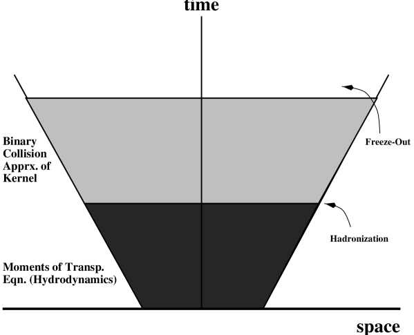
FIG. 1.: Schematic overview of the space-time evolution of a high-energy heavy-ion collision as assumed in the model presented here.

FIG. 2.: Schematic example of a hypersurface with both space-like and time-like parts.

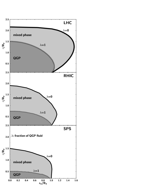
FIG. 3.: Hypersurfaces corresponding to $\lambda=1$ (boundary between pure QGP and mixed phase) and $\lambda=0$ (boundary between mixed phase and pure hadron phase) for LHC (top), RHIC (middle) and SPS (bottom).

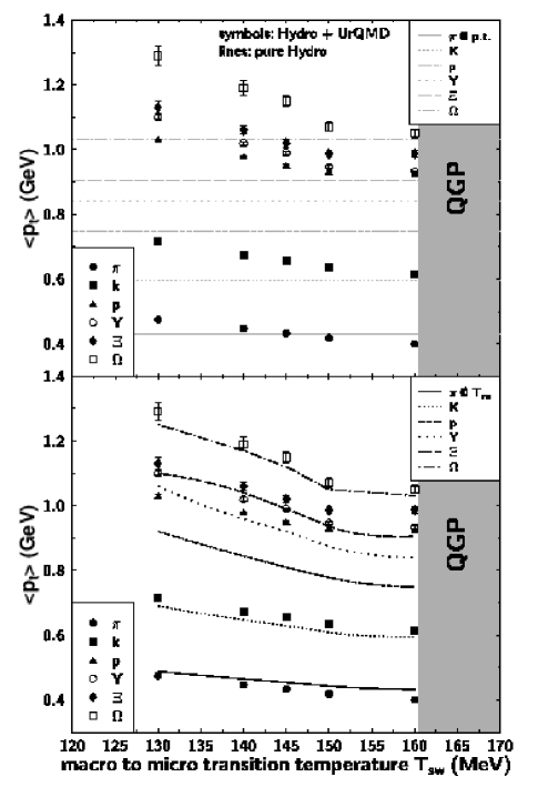
FIG. 4.: Mean transverse momentum $\langle p_{T}\rangle$ of various hadron species at freeze-out (symbols) vs. the macro to micro transition temperature $T_{sw}$. The horizontal lines in the upper frame show the respective $\langle p_{T}\rangle$ values right after hadronization ($\lambda=0$ hypersurface). The lines in the lower frame show the $\langle p_{T}\rangle$ emerging from ideal flow down to $T=T_{sw}$. This figure is for central $Au+Au$ collisions at BNL-RHIC energy.

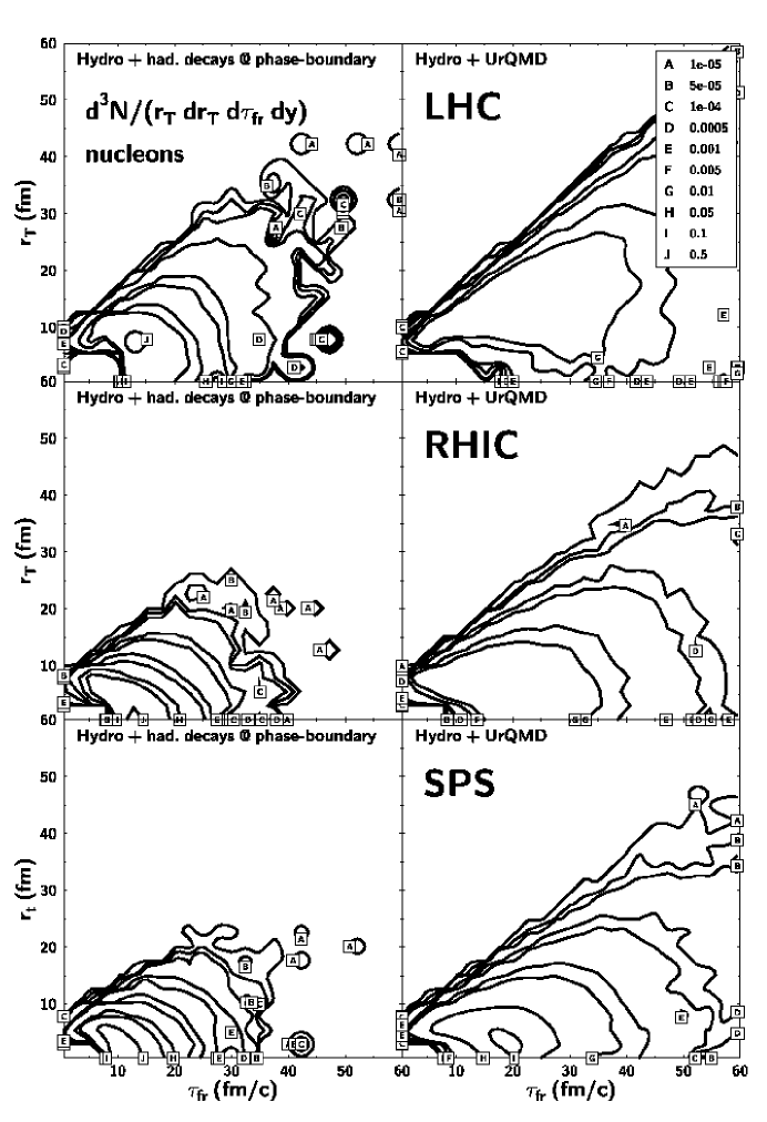
FIG. 5.: Freeze-out time and transverse radius distribution d${}^{3}N/(r_{T}$d$r_{T}$d$\tau_{fr}$d$y)$ for nucleons at LHC (top), RHIC (middle) and SPS (bottom). The left column shows the result for the pure hydrodynamical calculation up to hadronization with subsequent hadron resonance decays (but without hadronic reinteraction). The right column shows the analogous calculation, but with full microscopic hadronic collision dynamics after the hadronization. The contour lines have identical binning for all rows and columns.

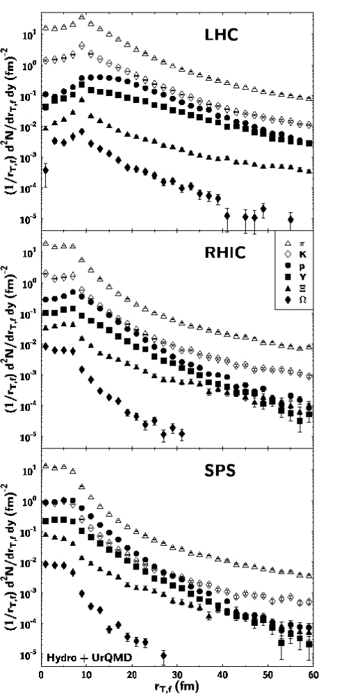
FIG. 6.: Transverse freeze-out radius distributions d${}^{2}N/r_{T,f}$d$r_{T,f}$d$y$ for various hadron species at LHC (top), RHIC (middle) and SPS (bottom).

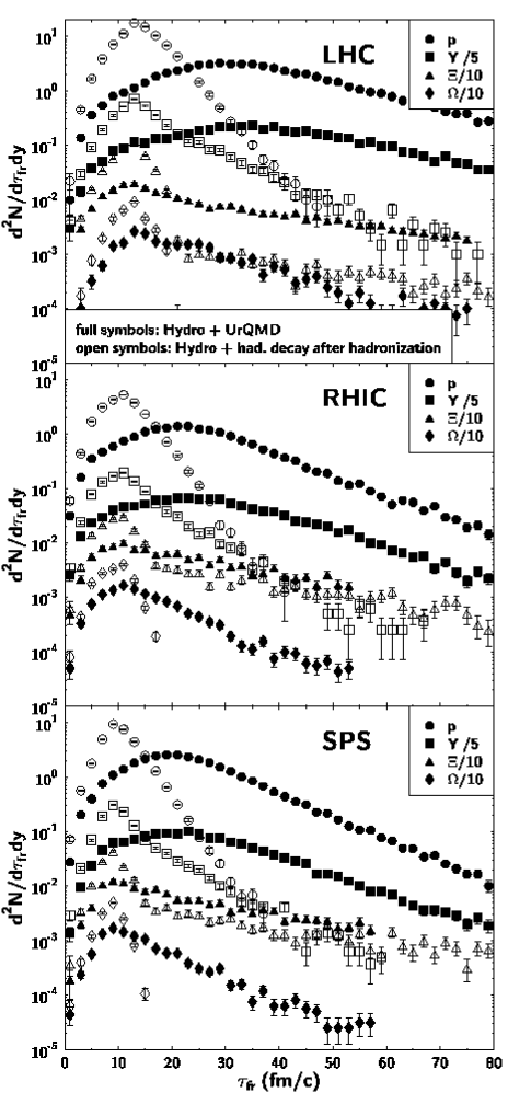
FIG. 7.: Freeze-out time distributions d${}^{2}N/$d$\tau_{fr}$d$y$ of $\pi$, $p$ and $\Omega^{-}$ for LHC (top), RHIC (middle) and SPS (bottom). Open symbols denote the distributions for a pure hydrodynamical calculation up to hadronization with subsequent hadron resonance decays (but without hadronic reinteraction), whereas the full symbols show the full calculation with hadronic rescattering.

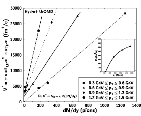
FIG. 8.: Estimated freeze-out volume of pions as a function of the pion rapidity density for four different bins in transverse momentum. High $p_{T}$-pions are only emitted from an outer shell, the radius of which increases with $p_{T}$. The inset shows the volume of the “hollow core” as a function of $p_{T}$.

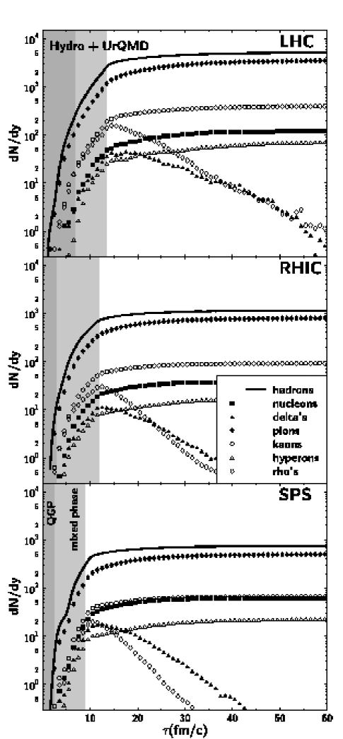
FIG. 9.: Time evolution of on-shell hadron multiplicities (integrated over $r_{T}$) at LHC (top), RHIC (middle) and SPS (bottom). The dark grey shaded area shows the duration of the QGP phase whereas the light grey shaded area depicts the coexistence phase.

FIG. 10.: Multiplicity change in % due to hadronic rescattering for various hadron species at SPS (bottom), RHIC (middle) and LHC (top). The error-bars give an estimate of the systematic error.

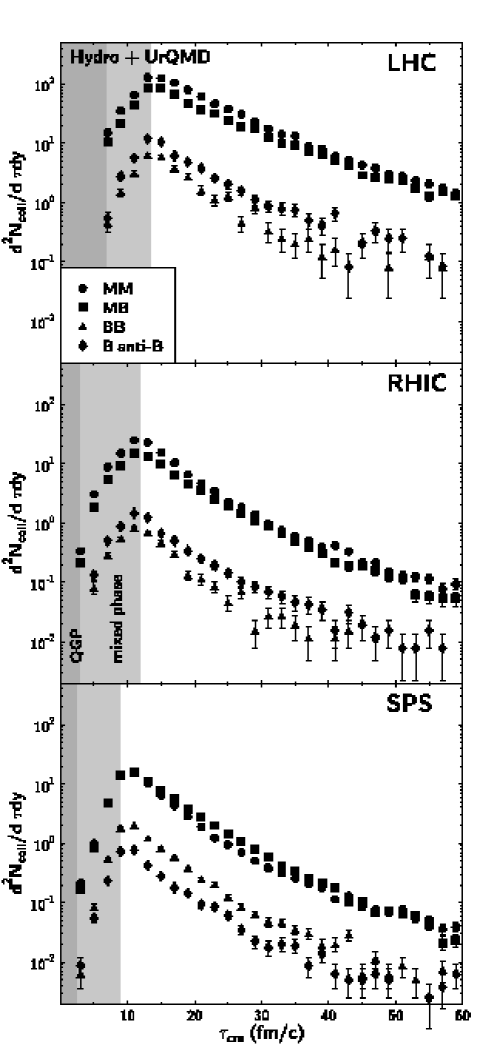
FIG. 11.: Hadron-hadron collision rates at LHC (top), RHIC (middle) and SPS (bottom). The dark grey shaded area shows the duration of the QGP phase whereas the light grey shaded area depicts the coexistence phase.

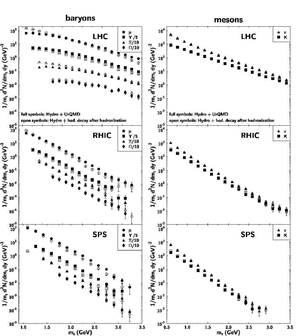
FIG. 12.: Transverse mass spectra of $\pi$, $K$ (left column) and $N$, $\Lambda+\Sigma^{0}$, $\Xi^{0}+\Xi^{-}$, and $\Omega^{-}$ (right column) at LHC (top), RHIC (middle) and SPS (bottom). The open symbols denote the spectra on the hadronization hypersurface whereas the full symbols show the calculation at freeze-out after hadronic rescattering.

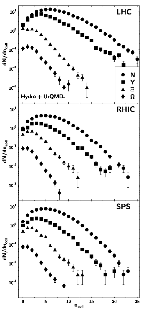
FIG. 13.: Distribution of the number of interactions that the final-state particles suffer after being hadronized; for LHC (top), RHIC (middle) and SPS (bottom).

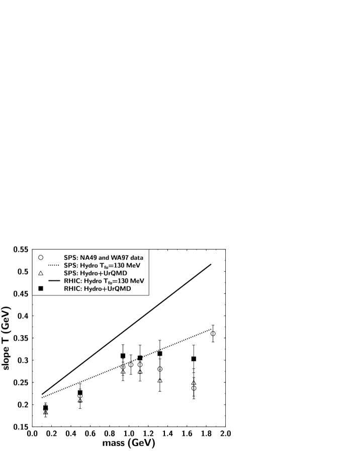
FIG. 14.: Inverse slopes of the $m_{T}$-spectra of $\pi$, $K$, $p$, $\Lambda+\Sigma^{0}$, $\Xi^{0}+\Xi^{-}$, and $\Omega^{-}$ at $y_{c.m.}=0$, $m_{T}-m_{i}<1$ GeV.

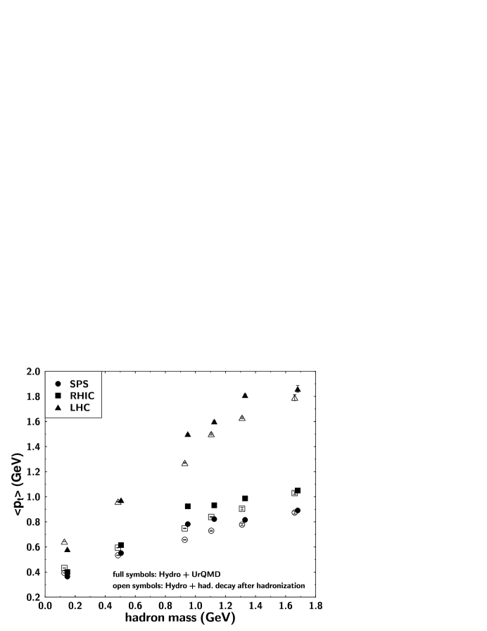
FIG. 15.: Average transverse momentum $\langle p_{T}\rangle$ vs. mass for $\pi$, $K$, $p$, $Y$, $\Xi$ and $\Omega$. The open symbols denote the spectra on the hadronization hypersurface (including strong resonance decays), the full symbols show the value at freeze-out (after hadronic rescattering). For clarity, the symbols have been shifted by $\pm 10$ MeV.

REFERENCES

- [1] E.W. Kolb and M.S. Turner, “The Early Universe”, Frontiers in Physics 69 (Addison-Wesley, Redwood City, USA, 1990)
-
[2]
J.C. Collins and M.J. Perry, Phys. Rev. Lett. 34,
1353 (1975);
E.V. Shuryak, Phys. Rept. 61, 71 (1980);
J. Rafelski, Phys. Rep. 88, 331 (1982); E. Witten, Phys. Rev. D30, 272 (1984);
L. McLerran, Rev. Mod. Phys. 58, 1021 (1986);
J. Cleymans, R.V. Gavai, and E. Suhonen, Phys. Rept. 130, 217 (1986);
B. Müller, Rept. Prog. Phys. 58, 611 (1995);
A.V. Smilga, Phys. Rept. 291, 1 (1997). -
[3]
J. Harris and B. Müller,
Ann. Rev. Nucl. Part. Sci. 46, 71 (1996);
S.A. Bass, M. Gyulassy, H. Stöcker and W. Greiner, J. Phys. G25, R1 (1999), e-print hep-ph/9810281. -
[4]
N.H. Christ and A.E. Terrano,
Phys. Rev. Lett. 56, 111 (1986);
F.R. Brown, N.H. Christ, Y.F. Deng, M.S. Gao, and T.J. Woch, Phys. Rev. Lett. 61, 2058 (1988);
Y. Iwasaki, K. Kanaya, S. Kaya, S. Sakai, and T. Yoshie, Phys. Rev. D54, 7010 (1996);
M. Oevers, F. Karsch, E. Laermann, and P. Schmidt, Nucl. Phys. Proc. Suppl. 63, 394 (1998); ibid. 73, 465 (1999) - [5] S.R. deGroot, W.A. van Leeuwen, and Ch.G. van Weert, “Relativistic Kinetic Theory” (North-Holland, Amsterdam, 1980).
-
[6]
B. Andersson, G. Gustafson, and C. Peterson,
Nucl. Phys. B135, 273 (1978);
K. Geiger, Phys. Rev. D47, 133 (1993);
T.S. Biro, P. Levai, and J. Zimanyi, Phys. Rev. C59, 1574 (1999);
C.T. Traxler, U. Mosel, and T.S. Biro, Phys. Rev. C59, 1620 (1999);
M. Hofmann, J.M. Eisenberg, S. Scherer, M. Bleicher, L. Neise, H. Stöcker, and W. Greiner, nucl-th/9908031. -
[7]
L.D. Landau and E.M. Lifshitz, “Fluid mechanics” (Pergamon,
New York, 1959);
for the application to nuclear collisions see e.g. R.B. Clare and D. Strottman: Phys. Rept. 141, 177 (1986);
for a pedagocical introduction see e.g. D.H. Rischke, Proceedings of the “11th Chris Engelbrecht Summer School in Theoretical Physics”, Cape Town, February 4–13, 1998, nucl-th/9809044. -
[8]
E. Shuryak, Phys. Rev. Lett. 68, 3270 (1992);
K. Geiger, Phys. Rev. D46, 4965 (1992). -
[9]
T.S. Biro, E. van Doorn, B. Müller, M.H. Thoma, and X.N. Wang,
Phys. Rev. C48, 1275 (1993);
K.J. Eskola and X. Wang, Phys. Rev. D49, 1284 (1994). - [10] S.M. Wong, Phys. Rev. C54, 2588 (1996).
-
[11]
H. Heiselberg and X. Wang, Nucl. Phys. B462, 389 (1996);
M. Gyulassy, Y. Pang, and B. Zhang, Nucl. Phys. A626, 999 (1997);
S.M. Wong, Phys. Rev. C56, 1075 (1997);
A.H. Mueller, hep-ph/9906322. - [12] K. Geiger and J.I. Kapusta, Phys. Rev. D47, 4905 (1993).
- [13] D.K. Srivastava, M.G. Mustafa, and B. Müller, Phys. Rev. C56, 1064 (1997).
- [14] D.M. Elliott and D.H. Rischke, nucl-th/9908004.
-
[15]
F.E. Low, Phys. Rev. D12, 163 (1975);
K. Kajantie and T. Matsui, Phys. Lett. B164, 373 (1985);
K.J. Eskola and M. Gyulassy, Phys. Rev. C47, 2329 (1993);
G.C. Nayak and V. Ravishankar, Phys. Rev. C58, 356 (1998). -
[16]
J. Letessier, A. Tounsi, U. Heinz, J. Sollfrank, and J. Rafelski,
Phys. Rev. Lett. 70, 3530 (1993);
P. Braun-Munzinger, J. Stachel, J.P. Wessels, and N. Xu, Phys. Lett. B365, 1 (1996);
J. Sollfrank, J. Phys. G23, 1903 (1997);
J. Cleymans and K. Redlich, Phys. Rev. Lett. 81, 5284 (1998);
C. Spieles, H. Stöcker, and C. Greiner, Eur. Phys. J. C2, 351 (1998);
J. Letessier and J. Rafelski, J. Phys. G25, 295 (1999). -
[17]
R. Stock, Phys. Lett. B456, 277 (1999);
U. Heinz, nucl-th/9907060. -
[18]
U. Ornik, M. Plümer, B.R. Schlei, D. Strottman, and R.M. Weiner,
Phys. Rev. C54, 1381 (1996);
B.R. Schlei, U. Ornik, M. Plümer, D. Strottman, and R.M. Weiner, Phys. Lett. B376, 212 (1996);
B.R. Schlei, Heavy Ion Phys. 5, 403 (1997);
N. Arbex, U. Ornik, M. Plümer, and R.M. Weiner, Phys. Rev. C55, 860 (1997). -
[19]
J. Sollfrank, P. Huovinen, M. Kataja, P.V. Ruuskanen,
M. Prakash, and R. Venugopalan, Phys. Rev. C55, 392 (1997);
J. Sollfrank, P. Huovinen, and P.V. Ruuskanen, Eur. Phys. J. C6, 525 (1999). -
[20]
U. Katscher, D.H. Rischke, J.A. Maruhn, W. Greiner, I.N. Mishustin,
and L.M. Satarov, Z. Phys. A346, 209 (1993);
A. Dumitru, U. Katscher, J.A. Maruhn, H. Stöcker, W. Greiner, and D.H. Rischke, Phys. Rev. C51, 2166 (1995). - [21] A. Dumitru and D.H. Rischke, Phys. Rev. C59, 354 (1999).
- [22] M. Prakash, M. Prakash, R. Venugopalan, and G. Welke, Phys. Rept. 227, 321 (1993).
- [23] P. Levai and B. Müller, Phys. Rev. Lett. 67, 1519 (1991).
- [24] P. Danielewicz and M. Gyulassy, Phys. Rev. D31, 53 (1985).
- [25] I. Mishustin and L. Satarov, Sov. J. Nucl. Phys. 37, 532 (1983).
- [26] C.M. Hung and E. Shuryak, Phys. Rev. C57, 1891 (1998).
- [27] A. Dumitru, Phys. Lett. B463, 138 (1999).
-
[28]
K.A. Bugaev, Nucl. Phys. A606, 559 (1996);
K.A. Bugaev and M.I. Gorenstein, nucl-th/9903072;
K.A. Bugaev, M.I. Gorenstein, and W. Greiner, nucl-th/9906088. -
[29]
C. Anderlik, Z.I. Lazar, V.K. Magas, L.P. Csernai, H. Stöcker,
and W. Greiner, Phys. Rev. C59, 388 (1999);
C. Anderlik, L.P. Csernai, F. Grassi, Y. Hama, T. Kodama, and Z.I. Lazar, Phys. Rev. C59, 3309 (1999);
V.K. Magas et al., Heavy Ion Phys. 9, 193 (1999). - [30] A. Dumitru, C. Spieles, H. Stöcker, and C. Greiner, Phys. Rev. C56, 2202 (1997).
-
[31]
F. Grassi, Y. Hama, and T. Kodama,
Z. Phys. C73, 153 (1996);
F. Grassi, Y. Hama, T. Kodama and O. Socolowski, Heavy Ion Phys. 5, 417 (1997);
F. Grassi and O.J. Socolowski, Phys. Rev. Lett. 80, 1170 (1998). -
[32]
L.V. Bravina, I.N. Mishustin, N.S. Amelin,
J.P. Bondorf, and L.P. Csernai,
Phys. Lett. B354, 196 (1995);
H. Sorge, Phys. Lett. B373, 16 (1996). - [33] S.A. Bass, A. Dumitru, M. Bleicher, L. Bravina, E. Zabrodin, H. Stöcker, and W. Greiner, Phys. Rev. C60, 021902 (1999).
- [34] S. Pratt and J. Murray, Phys. Rev. C57, 1907 (1998).
-
[35]
E. Andersen et al. (WA97 Collaboration),
Phys. Lett. B433, 209 (1998);
E. Andersen et al. (WA97 Collaboration), J. Phys. G25, 181 (1999). - [36] H. van Hecke, H. Sorge, and N. Xu, Phys. Rev. Lett. 58, 5764 (1998).
- [37] A. Dumitru, S.A. Bass, M. Bleicher, H. Stöcker, and W. Greiner, Phys. Lett. B460, 411 (1999).
- [38] F. Cooper and G. Frye, Phys. Rev. D10, 186 (1974).
- [39] S. Bernard, J.A. Maruhn, W. Greiner, and D.H. Rischke, Nucl. Phys. A605, 566 (1996).
-
[40]
S. A. Bass, M. Belkacem, M. Bleicher, M. Brandstetter, L. Bravina,
C. Ernst, L. Gerland, M. Hofmann, S. Hofmann, J. Konopka, G. Mao,
L. Neise, S. Soff, C. Spieles, H. Weber, L. A. Winckelmann,
H. Stöcker, W. Greiner, C. Hartnack, J. Aichelin and N. Amelin,
Progr. Part. Nucl. Physics Vol. 41, 225 (1998),
nucl-th/9803035
M. Bleicher, E. Zabrodin, C. Spieles, S.A. Bass, C. Ernst, S. Soff, L. Bravina, M. Belkacem, H. Weber, H. Stöcker and W. Greiner, J. Phys. G25, 1859 (1999) -
[41]
J.D. Bjorken,
Phys. Rev. D27, 140 (1983);
K. Kajantie and L. McLerran, Nucl. Phys. B214, 261 (1983). -
[42]
B. Kämpfer, Z. Phys. A353, 71 (1995);
A. Dumitru, U. Katscher, J.A. Maruhn, H. Stöcker, W. Greiner, and D.H. Rischke, Z. Phys. A353, 187 (1995) - [43] D.H. Rischke, S. Bernard, and J.A. Maruhn, Nucl. Phys. A595, 346 (1995).
- [44] D.H. Rischke and M. Gyulassy, Nucl. Phys. A597, 701 (1996).
- [45] A. Chodos, R.L. Jaffe, K. Johnson, C.B. Thorn, and V.F. Weisskopf, Phys. Rev. D9, 3471 (1974).
- [46] J. Cleymans, K. Redlich, and D.K. Srivastava, Phys. Rev. C55, 1431 (1997).
- [47] M. Belkacem, M. Brandstetter, S.A. Bass, M. Bleicher, L.V. Bravina, M.I. Gorenstein, J. Konopka, L. Neise, C. Spieles, S. Soff, H. Weber, H. Stöcker and W. Greiner, Phys. Rev. C58, 1727 (1998).
- [48] R.D. Pisarski and F. Wilczek, Phys. Rev. D29, 338 (1984).
- [49] M. Kataja, P.V. Ruuskanen, L.D. McLerran, and H. von Gersdorff, Phys. Rev. D34, 2755 (1986).
- [50] D.H. Rischke and M. Gyulassy, Nucl. Phys. A608, 479 (1996).
-
[51]
C.M. Hung and E. Shuryak,
Phys. Rev. Lett. 75, 4003 (1995);
T.S. Biro, nucl-th/9911004. -
[52]
K. Jedamzik, Phys. Rev. D55, R5871 (1997);
C. Schmid, D.J. Schwarz, and P. Widerin, Phys. Rev. Lett. 78, 791 (1997); Phys. Rev. D59, 043517 (1999);
K. Jedamzik and J.C. Niemeyer, Phys. Rev. D59, 124014 (1999). - [53] J. Brachmann, A. Dumitru, H. Stöcker, and W. Greiner, nucl-th/9912014.
-
[54]
T. Csörgö and B. Lörstad,
Phys. Rev. C54, 1390 (1996);
B. Kämpfer, O.P. Pavlenko, A. Peshier, M. Hentschel, and G. Soff, J. Phys. G23, 2001 (1997). - [55] J. Alam, D.K. Srivastava, B. Sinha, and D.N. Basu, Phys. Rev. D48, 1117 (1993).
-
[56]
L.P. Csernai and J.I. Kapusta, Phys. Rev. Lett. 69,
737 (1992);
L.P. Csernai, J.I. Kapusta, G. Kluge, and E.E. Zabrodin, Z. Phys. C58, 453 (1993);
J. Ignatius, K. Kajantie, H. Kurki-Suonio, and M. Laine, Phys. Rev. D49, 3854 (1994); D50, 3738 (1994). -
[57]
H. Heiselberg and A.D. Jackson, nucl-th/9809013;
O. Scavenius and A. Dumitru, Phys. Rev. Lett. 83, 4697 (1999). - [58] H. Appelshäuser et al., (NA49 collaboration), Phys. Rev. Lett. 82, 2471 (1999).
-
[59]
B. Müller and X.N. Wang,
Phys. Rev. Lett. 68, 2437 (1992);
B. Kämpfer and O.P. Pavlenko, Z. Phys. C62, 491 (1994);
K.J. Eskola and K. Kajantie, Z. Phys. C75, 515 (1997). -
[60]
T. Schönfeld, H. Stöcker, W. Greiner, and H. Sorge,
Mod. Phys. Lett. A8, 2631 (1993);
L. Gerland et al.,
e-print nucl-th/9512032;
S.E. Vance, M. Gyulassy, and X.N. Wang, Nucl. Phys. A638, 395c (1998). -
[61]
N. Hammon, H. Stöcker, and W. Greiner,
Phys. Rev. C61, 014901 (2000);
A. Krasnitz and R. Venugopalan, hep-ph/9909203. -
[62]
V. Emel’yanov, A. Khodinov, S.R. Klein, and R. Vogt, hep-ph/9909427;
K.J. Eskola, K. Kajantie, P.V. Ruuskanen, and K. Tuominen, hep-ph/9909456. - [63] C. Spieles, L. Gerland, H. Stöcker, C. Greiner, C. Kuhn, and J.P. Coffin, Phys. Rev. Lett. 76, 1776 (1996).
- [64] C.W. Misner, K.S. Thorne, and J.A. Wheeler, “Gravitation”, W.H. Freeman Press, San Francisco (1973)
-
[65]
Y. Yariv and Z. Fraenkel,
Phys. Rev. C20, 2227 (1979);
J. Cugnon, Phys. Rev. C22, 1885 (1980);
Y. Pang, T.J. Schlagel, and S.H. Kahana, Phys. Rev. Lett. 68, 2743 (1992). -
[66]
H. Kruse, B.V. Jacak, and H. Stöcker,
Phys. Rev. Lett. 54, 289 (1985);
J. Aichelin and G. Bertsch, Phys. Rev. C31, 1730 (1985);
J.J. Molitoris and H. Stöcker, Phys. Rev C32, R346 (1985);
K. Weber, B. Blattel, V. Koch, A. Lang, W. Cassing, and U. Mosel, Nucl. Phys. A515, 747 (1990);
B.A. Li and C. M. Ko, Phys. Rev. C52, 2037 (1995);
W. Ehehalt and W. Cassing, Nucl. Phys. A602, 449 (1996). -
[67]
J. Aichelin, A. Rosenhauer, G. Peilert, H. Stöcker, and W. Greiner,
Phys. Rev. Lett. 58, 1926 (1987);
G. Peilert, H. Stöcker, A. Rosenhauer, A. Bohnet, J. Aichelin, and W. Greiner, Phys. Rev. C39, 1402 (1989);
H. Sorge, H. Stöcker, and W. Greiner, Annals of Physics (N.Y.) 192, 266 (1989);
J. Aichelin, Phys. Rept. 202, 233 (1991). -
[68]
B. Andersson, G. Gustafson, G. Ingelman, and T. Sjöstrand,
Phys. Rept. 97, 31 (1983);
B. Andersson, G. Gustafson, and B. Nilsson-Almqvist, Nucl. Phys. B281, 289 (1987). -
[69]
F. Laue et al.,
Phys. Rev. Lett. 82, 1640 (1999);
W. Chang et al., nucl-ex/9904010. - [70] D. Zschiesche, P. Papazoglou, C.W. Beckmann, S. Schramm, J. Schaffner-Bielich, H. Stöcker and W. Greiner, nucl-th/9908072.
- [71] Particle-Data-Group, Phys. Rev. D54 (1996).
- [72] P. Danielewicz and G. F. Bertsch, Nucl. Phys. A533, 712 (1991).
- [73] E.V. Shuryak and O.V. Zhirov, Phys. Lett. 89B, 253 (1979); Phys. Lett. B171, 99 (1986).
-
[74]
Y. Sinyukov,
Z. Phys. C43, 401 (1989);
L.P. Csernai, Z.I. Lazar, and D. Molnar, Heavy Ion Physics 5, 467 (1997). -
[75]
S. Chapman, J.R. Nix, and U. Heinz,
Phys. Rev. C52, 2694 (1995);
U.A. Wiedemann, B. Tomasik, and U. Heinz, Nucl. Phys. A638, 475c (1997);
J.R. Nix, D. Strottman, H.W. van Hecke, B.R. Schlei, J.P. Sullivan, and M.J. Murray, nucl-th/9801045;
H. Appelshäuser et al. (NA49 Collaboration), Eur. Phys. J. C2, 661 (1998). - [76] S. Pratt, Phys. Rev. D33, 1314 (1986).
-
[77]
K. Geiger and B. Müller,
Nucl. Phys. B369, 600 (1992) 600;
K. Geiger, Phys. Rep. 258, 273 (1995);
K. Geiger, Comp. Phys. Com. 104, 70 (1997). - [78] S.A. Bass, M. Hofmann, M. Bleicher, L. Bravina, E. Zabrodin, H. Stöcker and W. Greiner, Phys. Rev. C60, 021901 (1999).
-
[79]
P.G. Jones and the NA49 collaboration,
Nucl. Phys. A610, 188c (1996);
C. Bormann et al., (NA49 collaboration), J. Phys. G23, 1817 (1997);
H. Appelshäuser et al., (NA49 collaboration), Phys. Lett. B444, 523 (1998). - [80] M. Bleicher, C. Spieles, C. Ernst, L. Gerland, S. Soff, H. Stöcker, W. Greiner, and S.A. Bass, Phys. Lett. B447, 227 (1999).
-
[81]
P.J. Siemens and J.O. Rasmussen, Phys. Rev. Lett. 42, 880 (1979);
H. Stöcker, A.A. Ogloblin, and W. Greiner, Z. Phys. A303, 259 (1981). - [82] I.G. Bearden et al., (NA44 Collab.), Phys. Rev. Lett. 78, 2080 (1997).
-
[83]
Y. Pang et al., http://rhic.phys.columbia.edu/oscar;
M. Bleicher, S.A. Bass, L.V. Bravina, W. Greiner, H. Stöcker, N. Xu and E. Zabrodin, hep-ph/9911420. - [84] I.N. Mishustin, Phys. Rev. Lett. 82, 4779 (1999)
- [85] M. Stephanov, K. Rajagopal, and E. Shuryak, Phys. Rev. D60, 114028 (1999)