Collective modes in asymmetric nuclei

Abstract

The collective motion of a finite nuclear system is investigated by numerical simulation and by linear response theory. Using a pseudo-particle simulation technique we analyze the giant resonances with a multipole decomposition scheme. We examine the energy and the damping of different giant collective modes and obtain the dependence of these quantities on the proton–neutron ratio. In simulations of finite nuclei including only mean fields the centroid energy of the resonance decreases with higher asymmetry due to the change of the compressibility and the damping increases. The collisional correlation in turn leads to a decreasing damping with increasing asymmetry.

Alternatively the giant collective modes in asymmetric nuclear matter are investigated within linear response theory including the collisional correlations via a dynamic relaxation time approximation. For a multicomponent system we derive a coupled dispersion relation and show that two sources of coupling appear: (i) a coupling of isoscalar and isovector modes due to the action of different mean-fields and (ii) an explicit new coupling in asymmetric matter due to collisional interaction. We show that the latter is responsible for a new mode arising besides isovector and isoscalar modes. The comparison with simulation results as well as experiments is performed. It is stressed that the surface effects and the collisional correlations are both essential in order to describe the correct damping behavior. A model is presented which allows to combine surface and collisional effects. Higher-order modes like the isoscalar dipole mode which where recently measured are discussed within this frame.

Collective motion beyond the linear regime is demonstrated for the example of large-amplitude isoscalar giant octupole excitations in finite nuclear systems. Depending on the initial conditions we observe either clear octupole modes or over-damped octupole modes which decay immediately into quadrupole ones. This dependence on initial correlations represents a behaviour beyond linear response.

Chapter 1 Introduction

Giant resonances are currently enjoying a resurgence of attention as a tool for the investigation of many particle effects in finite quantum systems. The study of giant resonances offers the possibility to learn more about nuclear forces. Of special interest are modern experiments with exotic nuclei which broaden our knowledge in a new degree of freedom: the variability in the proton to neutron ratio. The treatment of collective modes in nuclear matter is documented in an enormous literature starting from their discovery [1] up to recent discussions [2] -[35] and citations therein.

We want to investigate the collective excitations in asymmetric nuclear matter [6, 7] by numerical simulation of the Vlasov equation and by comparison with the linear response theory. While the former leads to an insight into finite-size effects like surface, the latter allows to consider collisional correlations in a control-able way. Both methods are contrasted and we demonstrate that the collisional correlations as well as the surface effects are important to describe the experimental damping of giant resonances.

The damping mechanisms of collective motions in excited nuclei are a topic of continuing debate. Mainly two lines of thought are pursued. In one line of thought it is assumed that collisions are the only physical reason for damping which is described via a Fermi liquid approach [6],[8]- [20, 36]. The other line of thought considers new features of the finite nucleus, such as surface oscillations and a level density with finite spacing. The investigations are performed without inertia [21]- [29, 37] or by including inertia [27],[30]- [35]; note that inertia is absent in infinite matter.

Both classes of models predict a comparable degree of damping necessary to reproduce the experimental data. Consequently, it is an open question which is the correct physical reason for damping. Of course, the correct description has to assume a finite nucleus consisting of nucleons which are bound via the mean field, through which the nucleons undergo mutual collisions and where the surface is formed by the particles themselves. These features are principally included in Boltzmann-Uehling-Uhlenbeck-(BUU) simulations [38, 39, 40] or in its nonlocal extensions [41, 42]. In full simulations, however, we will not gain a simple insight into the physical origins of the damping mechanism, in particular, how much is contributed by the surface and how much by collisions.

One aim of this article is therefore to compare both pictures in the frame of linear response theory. Within the collision-free Vlasov equation the linear response of finite systems is well known [43] and allows one to calculate the strength function of finite nuclei. The resulting damping, however, does not reproduce the experimental damping of giant resonances since collisions are absent. This motivates us to develop a linear response theory including collisions.

While most of the theoretical treatments of oscillations rely on the linear response method or RPA methods, large amplitude oscillations require methods beyond this level. In particular the question of the appearance of chaos has recently been investigated [44, 45, 46]. The hypothesis was established that the octupole mode is over-damped due to negative curved surface and consequent additional chaotic damping [47, 48, 49]. Here we want to discuss in which conditions one might observe octupole modes at least in Vlasov - simulations of giant resonances which will turn out to be dependent on initial conditions and are consequently an effect beyond linear response.

The outline is as follows: In the second chapter we will give the numerical results of pseudo-particle simulation of the Vlasov equation. This will provide us with some insight into the magnitude of finite size effects on the damping. In the third chapter we present the linear response result of the Vlasov equation including collisional correlations. We will consider a simplified picture of infinite matter response and will consider the Steinwedel Jensen picture. We discuss two possibilities to include surface contributions in the linear response formalism. This allows us to describe the experimental temperature dependence of the damping of giant dipole resonances as well as the structure function of the isovector dipole resonances. The surface consideration allows to describe the isoscalar dipole resonance as a higher order mode. The comparison between linear response results and simulations is performed and finally we discuss nonlinear effects beyond linear response for the example of giant octupole modes.

Chapter 2 Pseudoparticle simulation

We will describe the giant resonance first by a kinetic equation using a pseudo-particle simulation [50]. The kinetic equation for the quasiclassical distribution function reads for neutrons (for protons analogously)

$${\dot{f}}_{n}({\bf p,r},t)+\frac{{\bf p}}{m}{\bf\partial_{r}}f_{n}({\bf p,r},t)-{\bf\partial_{r}}(U_{n}+U_{\rm ext}){\bf\partial_{p}}f_{n}({\bf p,r},t)=I_{\rm corr}$$

with the collisional integral $I_{\rm corr}$ discussed later and the self-consistent mean-field potential $U$ given by a schematic Skyrme type [51]

$$U_{n/p}(\varrho,I) = a({\textstyle\frac{\varrho}{\varrho_{0}}})+b({\textstyle\frac{\varrho}{\varrho_{0}}})^{s}\pm cI({\textstyle\frac{\varrho}{\varrho_{0}}})$$ (2.2)

with $a=-356{\rm MeV}$, $b=303{\rm MeV}$ , $c=54{\rm MeV}$ and $s=7/6$. Here the neutron excess is $I=\frac{\varrho_{n}-\varrho_{p}}{\varrho_{n}+\varrho_{p}}$, the neutrons feel the +–sign potential, the protons the opposite one.

By multiplying the kinetic equation by $1,p$ or $E={p^{2}\over 2m}+U$ respectively one obtains the balance for particle density $\rho$, momentum density $u$ and energy density ${\cal E}$. Since the collision integrals vanish for density and momentum balance we get the usual balance equations

$${\partial\rho({\bf r},t)\over\partial t}+{\bf{\partial\over\partial r}}\int{d{\bf p}\over(2\pi\hbar)^{3}}{\partial E\over\partial{\bf p}}f({\bf p,r},t)=0$$

$${\partial u_{i}({\bf r},t)\over\partial t}+{\partial\over\partial r_{j}}\int{d{\bf p}\over(2\pi\hbar)^{3}}(p_{i}{\partial E\over\partial p_{j}}f({\bf p,r},t)+{\cal E}({\bf r},t)\delta_{ij})=0$$ (2.3)

where the mean field energy of the system varies as

$$\delta{\cal E} = \int{d{\bf p}\over(2\pi\hbar)^{3}}{\delta{\cal E}\over\delta f({\bf p,r},t)}\delta f({\bf p,r},t)$$ (2.4)

$$= \int{dp\over(2\pi\hbar)^{3}}({p^{2}\over 2m}+U)\delta f({\bf p,r},t)$$

such that from (2.2) follows the total energy density as

$${\cal E}({\bf r},t)=\int{d{\bf p}\over(2\pi\hbar)^{3}}{p^{2}\over 2m}f({\bf p,r},t)+{a\over 2}({\textstyle\frac{\varrho^{2}({\bf r},t)}{\varrho_{0}}})+{b\rho({\bf r},t)\over s+1}({\textstyle\frac{\varrho({\bf r},t)}{\varrho_{0}}})^{s+1}\pm{c\over 2}I({\textstyle\frac{\varrho^{2}({\bf r},t)}{\varrho_{0}}}).$$ (2.5)

With the help of this quantity the balance of energy density reads from (2)

$${\partial{\cal E}({\bf r},t)\over\partial t}+{\bf{\partial\over\partial r}}\int{d{\bf p}\over(2\pi\hbar)^{3}}E{\partial E\over\partial{\bf p}}f({\bf p,r},t)=-{\partial\over\partial t}E_{\rm corr}({\bf r},t)$$ (2.6)

with the correlation energy [52, 53] arising from the collisional side. The collisional side we will consider later in linear response. Here for the simulation we will neglect the collisions and will restrict ourselves to the Vlasov kinetic equation. In this way we will learn what are the effects of finite size and what are the effects of collisions.

Let us now first look at the input for the simulation. The mass number dependence of binding energy ${\cal E}/A$ from (2.5) is shown in figure 2.1. One sees that with increasing asymmetry the binding energy becomes weaker and consequently the compressibility decreases.

Figure 2.1: Left: Mass number dependence of the energy for different neutron excess $I=\frac{\varrho_{n}-\varrho_{p}}{\varrho_{n}+\varrho_{p}}$. The dots denote the saturation densities. With increasing asymmetry the saturation density and the binding energy decrease. Right: Asymmetry dependence of compressibility modulus. With increasing asymmetry this modulus decreases.

The compression modulus is defined as the derivative of the Energy per particle

$$K=9n^{2}{\partial({\cal E}/A)\over\partial n^{2}}$$ (2.7)

and took for $I=0$ the value $K=200\;{\rm MeV}$ according to (2.5). Figure 2.1 shows the asymmetry dependence of K. One sees that for neutron matter no binding energy would occur and a very low compressibility.

We solve now the kinetic equation by representing the distribution function $f({\bf p,r},t)$ by a sum of N pseudo-particle distributions

$$f({\bf p,r},t)\approx f_{0}({\bf p,r},t) = \sum\limits_{i=1}^{AN}\frac{1}{N}f_{S}({\bf p}-{\bf p_{i}}(t),{\bf r}-{\bf r_{i}}(t))\;$$ (2.8)

and use Gaussian pseudo-particles

$$f_{S}({\bf p-p_{1},r-r_{1}})=c\,\;e^{-({\bf p-p_{1}})^{2}/2\sigma_{p}^{2}}\;\;e^{-({\bf r-r_{1}})^{2}/2\sigma_{r}^{2}}$$ (2.9)

at ${\bf r_{1}}$ with momentum ${\bf p_{1}}$ [54]. These pseudo-particles follow classical Hamilton equations

$$\dot{\bf p}_{i} = -{\bf\nabla}U,\;\;\;\dot{\bf r}_{i}=\frac{{\bf p}_{i}}{m}\;.$$ (2.10)

The only fluctuations introduced are due to some small unavoidable numerical noise[55]. We are using 300 pseudo-particles per nucleon and a pseudo-particle width of $\sigma_{r}=0.466\;{\rm fm}$. They are adjusted both in such a way that the experimental energy of the ${}^{40}Ca$ giant monopole mode is reproduced. With these fixed two parameters the experimental behavior of centroid energy with mass number is than reproduced over the full range for giant monopole and giant dipole resonances. We have checked different numbers of test particles. The dependence of observables on the width is discussed in [56]. Numerically the ground states of nuclei are realized by Wood- Saxon shapes of density and Fermi spheres in momentum.

2.1 Multipole analysis

Provided we have now solved the kinetic equation we will have the distribution function represented by $N$ pseudo-particles. Since we are interested in moments of the distribution function, the density, current and energy, we can expand these moments in the test particle representation as well. The momentum distribution of these moments can be obtained by spatial integration: $F_{a}({\bf p})=\int d{\bf r}\,a\,f({\bf p,r})$ with, for the mass distribution, $a=1$, for isospin, $a=\tau$, for kinetic energy, $a=\frac{p^{2}}{2m}$, and for kinetic isospin energy, $a=\frac{\tau p^{2}}{2m}$ respectively. Decomposed into spherical coordinates they read

$$F_{a}(p,\vartheta,\varphi) = \sum_{i=1}^{AN}\frac{(2\pi)^{3}}{N}a_{i}\frac{\delta(p-p_{i})}{p_{i}^{2}}\delta(\varphi-\varphi_{i})\frac{\delta(\vartheta-\vartheta_{i})}{\sin(\vartheta_{i})}\;.$$ (2.11)

Radial integration determines now a spherical distribution

$$\bar{F}_{a}(\vartheta,\varphi) = \sum_{i=1}^{AN}\frac{1}{N}a_{i}\delta(\varphi-\varphi_{i})\frac{\delta(\vartheta-\vartheta_{i})}{\sin(\vartheta_{i})}$$ (2.12)

which can be decomposed into spherical harmonics

$$\bar{F}_{a}(\vartheta,\varphi) = \sum_{l=0}^{\infty}\sum_{m=-l}^{l}a_{lm}Y_{lm}(\vartheta,\varphi)\;,$$ (2.13)

$$a_{lm} = \sum_{i=1}^{AN}\frac{1}{N}a_{i}Y_{lm}^{\star}(\vartheta_{i},\varphi_{i}).$$ (2.14)

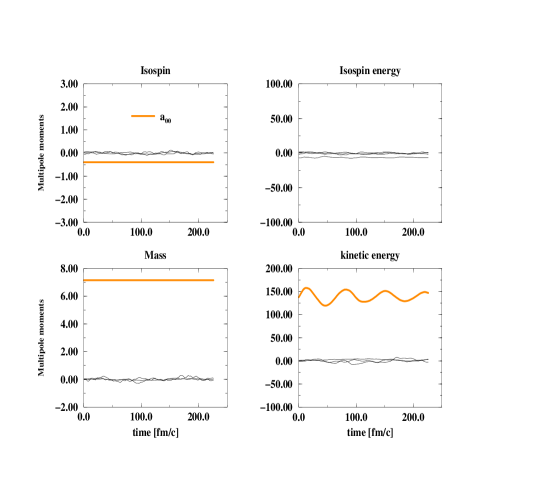
Figure 2.2: The picture shows for isoscalar monopole oscillations of ${}^{90}_{40}Zr$ the time evolution of multipole moments $\sqrt{\frac{2l+1}{4\pi}}a_{l0}(t),l=0,1,2,3$ corresponding to monopole, dipole, quadrupole and octupole oscillation for the distribution of isospin $a=\tau$, kinetic isospin energy $a=\frac{\tau p^{2}}{2m}$, mass $a=1$ and kinetic energy $a=\frac{p^{2}}{2m}$.

The observable distributions $\bar{F}_{a}(\vartheta,\varphi)$ are normalized to $\sqrt{4\pi}\;a_{00}$, i.e. to mass number $A$, total isospin $T$, kinetic energy $E_{kin}$ and kinetic isospin energy $E_{kinT}$, respectively. The polar angular distribution of moments reads now from (2.12) and (2.13)

$$\hat{F}_{a}(\vartheta)=\sum_{i=1}^{AN}\frac{1}{N}a_{i}\frac{\delta(\vartheta-\vartheta_{i})}{\sin(\vartheta_{i})}\equiv\int_{0}^{2\pi}d\varphi\,\bar{F}_{a}(\vartheta,\varphi) = \sum_{l=0}^{\infty}a_{l0}{\textstyle\sqrt{\frac{2l+1}{4\pi}}}P_{l}(\cos\vartheta)$$ (2.15)

with Legendre polynomials $P_{l}$. As a measure for the strength of the resonances we obtain now the coefficients $a_{l0}$ of the corresponding moment from (2.15) as

$$a_{l0}\sqrt{\frac{2l+1}{4\pi}}={2l+1\over 2}\sum_{i=1}^{AN}\frac{1}{N}a_{i}\frac{P_{l}(\cos\vartheta_{i})}{\sin(\vartheta_{i})}.$$ (2.16)

These amplitudes of multipole moments, $a_{l0}\sqrt{\frac{2l+1}{4\pi}}$, are displayed as a function of time in figures 2.2,2.5,2.8 and 2.9. The value $a_{10}$ means the dipole moment, vanishing for isoscalar resonances, $a_{20}$ is characterizing the quadrupole oscillations and $a_{30}$ the octupole ones, etc.

2.2 Isoscalar monopoles

The first analyzed mode is the isoscalar giant monopole mode which plays an important role in the determination of nuclear compressibility. The connection of the compressibility and the energy of giant monopole resonances is discussed e.g. in [57].

The figure 2.2 shows simulation results for a monopole oscillation. Here the excitation has been performed by adding an extra momentum to the test-particles in the direction of the center of mass. We have excited in this way a clear monopole breathing mode which can be seen in the oscillation of the kinetic energy. The corresponding mean field energy performs the opposite oscillations that the total energy is constant. The fact that energy is oscillating between kinetic and correlational ones describes why we have here a compressional or breathing mode. All other modes remain unexcited. The finite value of the isospin and mass for $l=0$ reflects the conservation of isospin and particle number.

With the previously chosen fixed width of test-particles we see from figure 2.3 that the experimental mass number dependence of monopole oscillation is well reproduced over the whole range of mass numbers. However, the experimental damping can be seen to be largely underestimated by the Vlasov simulation which yields about $2$ MeV. This is a first indication that the mean field, even for a finite system, cannot account for the whole damping and dissipation. Instead we have to take into account collisional correlations which will be performed later.

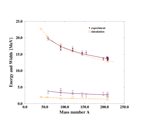
Figure 2.3: The mass number dependence of giant monopole oscillation energy and damping width. The solid line denotes the experimental values while the dashed line describes the Vlasov simulation results.

It is now instructive to examine the isospin dependence of the isoscalar monopole. Since this is the experimental value which determines the nuclear compressibility, the isospin dependence is of direct importance. In figure 2.4 the dependence on asymmetry of the isoscalar monopole energy is plotted for a hard as well as a stiff equation of state. Of course, the hard equation of state leads to a higher monopole energy corresponding to a higher compressibility. Analogously to figure 2.1 the monopole energy decreases with the asymmetry. The hard equation of state leads to a more linear decrease while the soft equation of state remains almost unchanged up to a certain asymmetry and then decreases faster.

Figure 2.4: The giant monopole energy (a) and normalized to the symmetric case (b) versus asymmetry for two different parameterizations of the mean field according to (2.6). The stiff equation of state (black line) leads to higher monopole energy and shows a more linear decrease while the soft equation of state (grey line) shows a weak dependence for small asymmetry and decreases faster for higher asymmetries.

2.3 Isovector dipole resonances

On the next figure 2.5 the multipole analysis for ${}^{90}_{40}Zr$ oscillations is performed. The excitation is now chosen as an isovector dipole one created by a shift of proton against neutron spheres. One recognizes that a clear dipole $a_{10}$ mode is excited which is seen in the oscillation of the isospin and isospin energy. The kinetic energy now remains constant in contrast to the isoscalar mode because we have no compression mode.

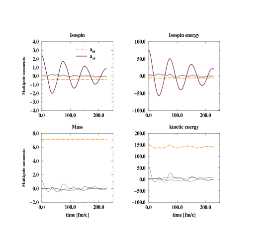
Figure 2.5: The time evolution of multipole moments for the isovector dipole excitation of ${}^{90}_{40}Zr$ analogously to figure 2.2.

Like the monopole case we now investigate the mass number dependence. With the same parameterization as for the monopoles, the experimental mass dependence of the energy is well reproduced, figure 2.6. The damping is again under-predicted. The Vlasov simulation leads to a nearly constant width of 2 MeV. This is again a hint that collisions cannot be neglected. The isospin dependency of the dipole mode is plotted in figure 2.7 and is characterized by an increasing width and decreasing centroid energy with increasing asymmetry.

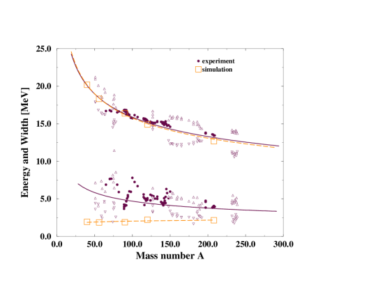
Figure 2.6: The experimental mass number dependence of isovector giant dipole oscillations (upper curve) is compared with the Vlasov simulation results. The oscillations in the experimental damping width are due to shell closures.

Figure 2.7: The isospin dependency of the centroid energy and the damping of the isovector dipole (left), isoscalar quadrupole (middle) and isovector quadrupole mode (right).

2.4 Quadrupole resonances

Let us now investigate the quadrupole resonances. For these we distinguish isoscalar and isovector modes. The quadrupole resonances are excited by dividing the spatial distribution into two equal pieces which are accelerated in opposite directions. In the first example the neutrons and protons are in phase giving rise to an isoscalar mode.

We see from the kinetic energy in figure 2.8 that besides the clear isoscalar quadrupole mode there is also a weak isoscalar monopole mode excited. The isospin dependency of the isoscalar quadrupole mode is plotted in figure 2.7. As in the case of the isovector dipole mode one sees a slight decrease of the centroid energy and an increase of damping with increasing asymmetry.

In the second case we excite protons and neutrons out of phase which excites isovector quadrupole oscillations in figure 2.9. The isospin energy and the isospin show nice oscillations in the quadrupole multipole moment. There is a slight excitation of an isovector dipole mode too. We would like to remark that due to the test particle width there occurs a mode coupling [56] which can be seen in the slight excitation of isoscalar modes in the kinetic energy. The isospin dependence shown in figure 2.7 has the same qualitative behaviour as the isoscalar mode, but is stronger in this case.

Figure 2.8: The time evolution of multipole moments for the isoscalar quadrupole excitation of ${}^{90}_{40}Zr$ analogously to figure 2.2.

Figure 2.9: The time evolution of multipole moments for the isovector quadrupole excitation of ${}^{90}_{40}Zr$ analogously to figure 2.2.

Chapter 3 Collective modes in linear response

Now we would like to focus on small amplitude oscillations and we will develop the linear response theory. Large amplitude motions and effects beyond linear response are discussed in chapter 4. The simplest microscopic theory which provides basic experimental features and which allows to include collisional correlations is the Fermi-gas(liquid) model including dissipation. We will compare the results from this linear response with the simulation of finite nuclei, and both will be compared with the experimental data.

The principle of linear response is easily explained. When a system which is described by the kinetic equation (2) is disturbed by an external potential $U^{\rm ext}$ it will react and will create a density change ${\delta\rho}$. The connection of the latter to the external perturbation is called the response function, ${\delta\rho}=\chi U^{\rm ext}$. Without mean field in (2) we would obtain the polarization $\Pi$ of the system. The mean field introduces a selfconsistency such that the relation between response function and polarization becomes

$$\chi={\Pi\over 1-{\delta U\over\delta n}\Pi}$$ (3.1)

where we have assumed that the mean field $U$ is only density dependent. Therefore the potential for the response function is $V={\delta U\over\delta n}$. The collective mode of a system is now characterized by the condition that the denominator in (3.1) vanishes

$$\epsilon({\bf q},\omega)=1-V({\bf q})\Pi({\bf q},\omega)=0$$ (3.2)

since then an infinitesimal small external potential can create a finite density oscillation due to the diverging response function. Therefore we will search for complex zeros of the dielectric (or dinuclic) function (DF), $\epsilon({\bf q},\Omega+i\gamma)=0$, which provides us with the energy $\Omega$ and the damping $\gamma$ of the collective mode. The strength function is then given by

$$S({\bf q},\omega)=\displaystyle{\frac{1}{\pi}{{\rm Im}\Pi\over(1-V{\rm Re}\Pi)^{2}+(V{\rm Im}\Pi)^{2}}}.$$ (3.3)

The equation of state like the isothermal compressibility can be expressed by

$$\kappa={1\over n^{2}}\left({\partial n\over\partial\mu}\right)_{T}={1\over n^{2}T}\lim\limits_{q\to 0}\int{d\omega\over\pi}{1\over{\rm e}^{\omega/T}-1}{\rm Im}{\chi(q,\omega)}$$

(3.4)

and the fluctuations and diffusion coefficients can also be expressed via the response function.

Two lines of theoretical improvements of the response function can be found in recent publications. The first one starts from TDHF equations and considers the response of nuclear matter described by a non time-reversal Skyrme interaction [14, 58, 59]. The other line tries to improve the response by the inclusion of collisional correlations [60, 61, 62, 63, 64] and by considering multicomponent systems [18, 65, 66, 67, 68]. In [64] both lines of improvements have been combined into one expression. We follow this line and derive the response function from a kinetic equation including mean field (Skyrme) and collisional correlations. Therefore we consider interacting matter which can be described by an energy functional ( mean field) ${\cal E}$ originally introduced by Skyrme [69, 70] and the residual interaction. The latter we condense in a collisional integral additional to the TDHF equation. Then the response to an external perturbation will contain the effect of Skyrme mean field and additionally the effect of the residual interaction.

3.1 Response function for asymmetric matter

The system now consists of a number of different species (neutrons, protons, etc…) interacting with their own kind and with the others. It is important to consider the interaction between different sorts of particles if we want to include friction between different streams of isospin components, etc. In particular the isospin current may not be conserved in this way. Let us start with a set of coupled quantum kinetic equations for the reduced density operator $\hat{\rho}_{a}$ of a certain species denoted by the subscript $a$

$$\partial_{t}\hat{\rho}_{a}(t)=i[\hat{\rho}_{a},{\hat{E}}_{a}(t)+{\hat{U}}_{a}^{\rm ext}]-\sum\limits_{b}\int\limits_{0}^{t}dt^{\prime}{\hat{\rho}_{a}(t^{\prime})-\hat{\rho}_{b}^{\rm l.e.}(t^{\prime})\over\tau_{ab}(t-t^{\prime})}$$ (3.6)

where ${\hat{E}}={\hat{P}}^{2}/2m+{\hat{U}}$ denotes the kinetic as well as mean field energy operator and the external field which is assumed to be a nonlinear function of the density. We approximate the collision integral by a non-Markovian relaxation time which is derived in appendix A. This turned out to be necessary to reproduce damping of zero sound [71, 72]. It accounts for the fact that during a two-particle collision a collective mode can couple to the scattering process. Consequently, the dynamical relaxation time represents the physical content of a hidden three-particle process and is equivalent to memory effects.

Furthermore, we assume relaxation towards a local equilibrium

$$f_{a}^{\rm l.e.}({\bf p,R},t)=\sum\limits_{q}{\rm e}^{i{\bf qR}}\langle p+{q\over 2}|\hat{\rho}_{a}^{\rm l.e.}|p-{q\over 2}\rangle=f_{0}\left({\varepsilon_{a}({\bf p}-{\bf Q}_{a}({\bf R},t))-\mu_{a}({\bf R},t)\over T_{a}({\bf R},t)}\right)$$ (3.7)

with the Fermi distribution $f_{0}$. This local equilibrium will be specified here only by a small deviation of the chemical potential of species $a$ ensuring density conservation [64]. The extension of the method including further conservation laws and specifying also the local current and the temperature can be found in [64].

Linearizing the kinetic equation (3.6) we obtain the matrix equation for the density deviation $\delta\rho_{b}$ due to an external perturbation $U^{b}_{\rm ext}$

$$\sum\limits_{b}\delta n_{b}\left\{\delta_{ab}-{i\over\omega\tau_{a}+i}\left[\delta_{ab}-{\tau_{a}\over\tau_{b}}C_{ab}\right]-\Pi_{a}(\omega+{i\over\tau_{a}})\alpha_{ab}\right\}=\Pi_{a}(\omega+{i\over\tau_{a}})U_{\rm ext}^{a}.$$ (3.8)

The matrix $C_{ab}$ is given by

$$C_{ab}=\sum\limits_{c}\left\{1\over\tau\right\}_{ac}{\Pi_{c}\Big{[}(\omega+{i\over\tau_{a}})\frac{m_{a}}{m_{c}}\Big{]}\over\Pi_{c}(0)}\left\{\frac{1}{\tau}\right\}^{-1}_{cb}$$ (3.9)

with $\alpha_{ab}={\partial\over\partial\,\rho_{b}}U_{a}$ the linearization of the mean field with respect to the deviation of density from equilibrium value caused by the external perturbation $U_{\rm ext}$. The partial polarization function of species $a$ is

$$\Pi_{a}(\omega)=2\int{dp\over(2\pi)^{3}}\frac{f_{a}(p+\frac{q}{2})-f_{a}(p-\frac{q}{2})}{\epsilon_{a}(p+\frac{q}{2})-\epsilon_{a}(p-\frac{q}{2})-\omega+i0}.$$ (3.10)

The factor 2 in front of the integral accounts for the spin degeneracy according to $\rho_{a}=2\int{dp\over(2\pi)^{3}}f_{a}(p)$.

Equation (3.8) represents the complete polarization of the system, because $\delta\rho=\Pi\,U_{\rm ext}$. It represents a matrix equation which is solved easily. The collective modes are given by the zeros of the determinant of the matrix on the left hand side of (3.8) because these are the poles of the polarization matrix. Since we took into account relaxation processes between all species we are able to cover current - current friction. For a two component system, e.g. neutrons with density $\rho_{n}$ and protons with density $\rho_{p}$, we write explicitly

$$(1-\Pi_{n}^{\rm M}\alpha_{nn})(1-\Pi_{p}^{\rm M}\alpha_{pp})-(D_{np}+\Pi_{n}^{\rm M}\alpha_{np})(D_{pn}+\Pi_{p}^{\rm M}\alpha_{pn})=0$$ (3.11)

with the generalization of the Mermin polarization function [73] to a multicomponent system

$$\Pi_{a}^{\rm M}={\Pi_{a}(\omega+{i\over\tau_{a}})\over 1-{i\over\omega\tau_{a}+i}(1-C_{aa})},$$ (3.12)

and the additional coupling due to asymmetry in the system

$$D_{np}={\tau_{n}\over\tau_{p}}{C_{np}\over C_{nn}-i\omega\tau_{n}}.$$ (3.13)

The $D_{pn}$ are given by interchanging species indices. This term does not appear for symmetric matter. Therefore we call this term the asymmetry coupling term further on. The result (3.11) represents the generalization of the dispersion relation (3.2) to a two - component system.

It is illustrative to recover known results for symmetric nuclear matter. This is performed for the case of equal relaxation times $\tau_{p}=\tau_{n}=\tau$ and equal deviation from the mean field $\alpha_{1}=\alpha_{nn}=\alpha_{pp}$ and $\alpha_{2}=\alpha_{np}=\alpha_{pn}$. Eq. (3.11) takes then the known Mermin form of dispersion relation [73]

$$1-(\alpha_{1}\pm\alpha_{2}){\Pi(\omega+{i\over\tau})\over 1-{i\over\omega\tau+i}\left[1-{\Pi(\omega+{i\over\tau})\over\Pi(0)}\right]}=0$$ (3.14)

with the isovector mode $\alpha_{1}-\alpha_{2}$ and the isoscalar mode $\alpha_{1}+\alpha_{2}$. Please note that for zero temperature the Mermin expression (3.14) agrees with the response function derived from taking into account multipole expansion in momentum of the disturbed distribution [36].

We have presented a general dispersion relation for the multicomponent system including known special cases. The dispersion relation (3.11) is similar to the one derived recently in [67, 74] if we neglect the collisional coupling $D_{np}$. Also a more general polarization function (3.12) is presented here including collisions within a conserving approximation [60]. In the following we will apply this expression to the damping of giant dipole resonances in symmetric as well as asymmetric nuclear matter.

3.2 Application to nuclear matter

Before we can solve the dispersion relation (3.11) we have to specify the wave vector characteristic of the considered mode. This is performed according to the Steinwedel-Jensen [75] model. We assume that the surface remains constant and the density oscillation obeys a wave equation with the boundary condition that the radial velocity vanishes on the spherical surface with radius $R=1.13A^{1/3}$. This leads to $j_{l}^{\prime}(kR)\equiv 0$ with the spherical Bessel function of order $l=0,1...$ associated with the monopole, dipole… resonances. From this condition one obtains a connection between the wave vector and the radius of the nuclei or the mass number in the form

$$k_{i,l}={c_{il}\over 1.13A^{1/3}}$$ (3.15)

for the $i$-th mode of multipolarity $l$ where $c_{il}$ is the $i$-th zero of $j_{l}^{\prime}(c)\equiv 0$.

For the monopole modes as compression modes we have no zero of first order for $l=0$. For the dipole modes one has in first order $k=2.08/R$ which describes the giant isovector dipole resonance (IVGDR) while the ISGDR is a spurious mode in first order. This would just mean an unphysical oscillation of center of mass motion. However, in second order $k=5.94/R$ the isoscalar giant dipole resonance (ISGDR) has been observed recently ([76] and references therein). This can be considered as a density oscillation inside a sphere as we will discuss in chapter 3.6.

Besides the occurring wave vector we have also to specify the relaxation times which contain the effect of collisions. The dynamic relaxation time has been derived by Sommerfeld expansion [6] in appendix A as

$${1\over\tau_{ab}^{\rm gas}(\omega)} = {1\over\tau_{ab}(0)}\left[1+\frac{3}{4}\left({\omega\over\pi T}\right)^{2}\right]\qquad\qquad{1\over\tau_{ab}^{\rm liq}(\omega)}={2\over\tau_{ab}(0)}\left[1+\frac{1}{2}\left({\omega\over\pi T}\right)^{2}\right]$$ (3.16)

for $a,b$ neutrons or protons respectively and dependent on whether we use a Fermi liquid or Fermi gas model. The Markovian relaxation time is given in terms of the cross section $\sigma_{ab}$ between species $a$ and $b$ as $\tau^{-1}_{ab}={4m\over 3\hbar^{3}}\sigma_{ab}T^{2}$.

We will use as an illustrative example a slightly different mean field potential than (2.2) given by [77, 78]

$$U_{a}=t_{0}\left[(1+{x_{0}\over 2})(\rho_{n}+\rho_{p})-(x_{0}+\frac{1}{2})\rho_{a}\right]+{t_{3}\over 4}\left[(\rho_{n}+\rho_{p})^{2}-\rho_{a}^{2}\right]$$ (3.17)

with $a=n,p$ the density of neutrons or protons respectively. The Coulomb interaction leads to an additional contribution for the proton mean-field

$$U_{p}^{C}(q)={4\pi e^{2}\over q^{2}}\rho_{p}(q).$$ (3.18)

The model parameters used here reproduce the Weizsäcker formula

$${{\cal E}\over A}=-a_{1}+{a_{2}\over A^{1/3}}+{a_{3}Z^{2}\over A^{4/3}}+a_{4}I^{2}$$ (3.19)

with the volume energy $a_{1}=15.68$ MeV, Coulomb energy $a_{3}=0.717$ MeV and the symmetry energy $a_{4}=28.1$ MeV with the asymmetry parameter $I={n_{n}-n_{p}\over n_{n}+n_{p}}$.

Figure 3.1: The experimental centroid energies (A) and damping rates (B) [filled symbols] of the giant dipole resonances vs mass number (data from Ref. [79]) together with different approximations at $T=0$.

The energy and damping rates are now determined by the zeros of the (Mermin) polarization function (3.14). First we plot the solution of the dispersion relation (3.11) for symmetric nuclear matter. In figure 3.1 we have plotted the real and imaginary (FWHM) part of complex energy for different approximations with relaxation time (collisions) and with and without Coulomb mean field (3.18). In figure 3.1 (A) we find that the inclusion of Coulomb effects reproduces the experimental shape of the centroid energies at higher mass numbers (dot-dashed line). Taking only collisions into account fails to describe higher mass numbers (solid line). Considering Coulomb together with collisions (dashed line), the centroid energies are reduced towards the data.

The experimental values of the damping rates are also presented versus mass number (figure 3.1 (B)). We recognize that the FWHM is just twice the damping rate $\Gamma=2\gamma$ which has been recently emphasized [15]. It has to be stressed that the experimental data are accessible by this FWHM. Here we have considered only collisions and have a vanishing Landau damping for the infinite matter model [6].

3.3 Comparison between simulation and linear response

We have already stressed that the simulation of finite nuclei neglecting collisional correlations lead to a damping of about $\Gamma_{\rm Land}=2$MeV for the giant dipole resonance at zero temperature. This was attributed to the surface effects of spherical symmetric nuclei. We consider this as the numerical value of the contribution attributed to the wall [36] at zero temperature. For finite temperature the will be considered an additional contribution due to thermally deformed shapes in section 3.5. Nevertheless it is now interesting to compare the isospin dependences of the simulation without collisions and the linear response including collisions but no surface effects.

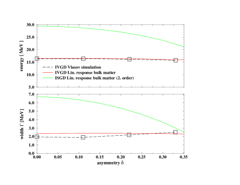
Figure 3.2: The dependence of isovector dipole resonance energy and damping on the asymmetry obtained from simulations and from linear response for $A=90$.

In figure 3.2 we see that the damping is slightly increasing with increasing asymmetry for simulations without collisions while the collisional contributions cause a slight decrease of damping. This decrease is much more pronounced in the second order isoscalar dipole mode. The energy in turn shows the same behaviour for simulations without correlations and for linear response with correlations; it slightly decreases the value.

The same qualitative feature can be recognized for the quadrupole modes in figure (3.3). However the importance of collisional damping is in this case much larger than the finite size effects.

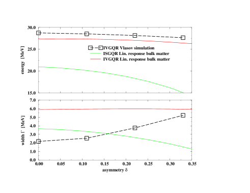
Figure 3.3: The dependence of isovector and isoscalar quadrupole resonance energy and damping on the asymmetry obtained from simulations and from linear response for $A=90$.

3.4 Giant resonances in excited nuclei

We consider now the temperature dependence of the GDR. We have found that the centroid energy only slightly decreases with increasing energy. In Fig. 3.4 the theoretical damping rates $\Gamma=2\,\gamma$ of the IVGDR modes in ¹²⁰Sn and ²⁰⁸Pb are plotted as a function of temperature together with experimental values. The results of the Fermi gas model (A.11) and the Fermi liquid model (A.19) are very close and in good agreement with the data at low temperature. The higher temperature dependence still remains too flat compared to the experiments. The small difference between both models for T=0 vanishes with increasing temperature.

Figure 3.4: Experimental damping rates vs. temperature of IVGDR for ¹²⁰Sn and ²⁰⁸Pb (¹²⁰Sn from Ref. [80] and ²⁰⁸Pb from Ref. [81]) compared with the solution of the dispersion (3.14) relation $\Gamma=2\,\gamma$ for the Fermi gas (dashed lines) and the Fermi liquid model (solid lines). Please note that this damping is reduced when the momentum conservation is included like it is done in figure 3.5.

While the figures indicate that the linear response including collisional correlations together with the Steinwedel Jensen model can describe quite well the gross features of giant dipole resonances we should keep in mind that we have neglected here the surface effects. From the simulation results of the second chapter we have seen that there is a damping of about $\Gamma_{\rm Land}=2$MeV for finite nuclei at zero temperature without collisional correlations. Simply adding now both contributions would overestimate the experimental damping. We would like to point out that the inclusion of only density conservation in the derivation of the response function so far is overestimating the width. In [64] we have shown that the inclusion of momentum conservation reduces this width by approximately $2$MeV. Therefore we might anticipate that both the finite size effects together with the collisional contribution lead to the correct value for low temperatures.

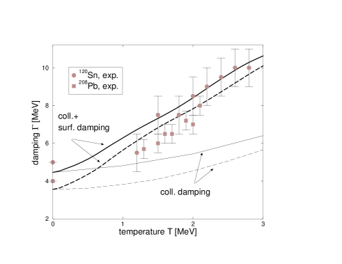
Figure 3.5: The effective damping consisting of only collisional damping compared with collisional and surface damping [¹²⁰Sn (solid lines) and ²⁰⁸Pb (dashed lines)] together with the experimental data (filled symbols: Sn from Ref. [80] and Pb from Ref. [81]).

In figure 3.5 we see that the temperature increase is too flat compared to the experimental finding if we consider only collisional damping (thin lines). From simulation results of ground state we have already found a contribution from finite size effects. We might now expect that the discrepancy in temperature behaviour is due to finite size effects. This should be explained and understood within a more simplified model.

3.5 Nuclear surface contribution - excited nuclei

Besides the $\Gamma_{\rm Land}=2$MeV of the simulation in the ground state we can have additional damping due to shape deformation if we increase the temperature. In Ref. [82] we have presented a method to include also scattering with the non-spherical nuclear surface. This improves the temperature dependence remarkably (thick lines) in figure 3.5.

The idea is to consider the surface scattering contribution to the damping determined by the additional Lyapunov exponent due to the surface. It has been shown that such Lyapunov exponents appear in the response function additive to the frequency as imaginary shift provided the Lyapunov exponent is small compared to the product of wave vector times Fermi velocity [82, 83]

$$\Pi_{0}^{\rm surf}(q,R,\omega)=\Pi_{0}^{\rm inf}(q,p_{f}(R),\omega+i\lambda).$$ (3.20)

The Lyapunov exponent by itself is calculated for different deformations of the surface corresponding to different temperatures

$$R_{\lambda}(\theta)=R_{0}\,\left(1+\alpha_{00}+\alpha_{\lambda}\,P_{\lambda}(\cos{(\theta)})\right)$$ (3.21)

with the nuclear radius $R_{0}=1.13A^{1/3}$fm, and where $\lambda=2$ corresponds to the quadrupole and $\lambda=3$ to the octupole deformation [84]. The corresponding mean deformation is linked to the temperature

$$\langle\alpha\rangle={\int d\alpha|\alpha|\exp{(-E_{B}(\alpha)/T)}\over\int d\alpha\exp{(-E_{B}(\alpha)/T)}}$$ (3.22)

where the surface dependent energy $E_{B}(\alpha)$ is given by the Bethe-Weizsäcker formula

$${E_{B}}(\alpha)=-a_{1}+{a_{2}\over A^{1/3}}+{a_{3}Z^{2}\over A^{4/3}}+a_{4}I^{2}+a_{5}A^{2/3}{S(\alpha)\over S(0)}$$

with the volume energy $a_{1}=15.68$ MeV, Coulomb energy $a_{3}=0.717$ MeV, the symmetry energy $a_{4}=28.1$ MeV and the surface energy $a_{5}=18.56$ MeV. For the quadrupole, $S_{2}$, and octupole, $S_{3}$, deformations one gets

$${S_{2}(\alpha)\over S(0)} = 1+\frac{2}{5}\alpha^{2}+{\cal O}(\alpha^{3})$$

$${S_{3}(\alpha)\over S(0)} = 1+\frac{5}{7}\alpha^{2}+{\cal O}(\alpha^{3}).$$ (3.24)

This represents the lowest order expansion in $\alpha$, however the next term gives already corrections in fractions of percent for the highest deformations considered here. By this way, the statistical model (3.22) leads to a connection between temperature and deformation as

$$T=c\pi a_{5}A^{2/3}<\alpha>^{2}$$ (3.25)

where the constant $c$ is given by the coefficient of $\alpha^{2}$ in Eq. (3.24) for the corresponding quadrupole or octupole deformation.

Using Eq. (3.25) we can translate the Lyapunov exponent $\lambda$ calculated as a function of deformation into a function of the temperature. In figure 3.6 the contribution to the damping of IVGDR for ¹²⁰Sn (circles) and ²⁰⁸Pb (squares) is presented for different shape deformations versus temperature. If we add quadrupole and octupole deformations we come up with a damping curve very similar to [27]. The damping starts at zero and increases rapidly with increasing temperature. We see that the main contribution comes from the quadrupole deformation while the octupole deformation is only sizeable at higher temperature. Let us note that the qualitative difference between Sn and Pb is reproduced by including surface scattering as well as collisional damping.

Figure 3.6: The scaled collisional damping is compared with the damping according to the chaotic scattering from the surface of quadrupole and octupole deformed shapes for ¹²⁰Sn and ²⁰⁸Pb.

The collisional contribution $\Gamma=2\gamma$ is plotted as well (Sn: solid line, Pb: dashed line). We recognize that both contributions by themselves, collisional as well as surface scattering, account almost for the same amount required by the experimental values, see figure 3.6. A proper relative weight between both processes is therefore necessary which will be introduced in the following.

Let us note before that we have considered the surface contribution to the damping for a deformed surface by temperature which therefore vanishes at zero temperature. However, for a spherical surface we got already from simulation a zero temperature contribution of $\Gamma_{\rm Land}=2$MeV. Consequently for the total damping caused by surface both contribute.

So far we have not considered that only particles close to the surface can appreciably contribute to the surface scattering and to this chaotization process, while particles deep inside the nuclei are screened out of this process. Consequently we consider the corresponding collision frequencies as the measure to compare surface collisions with inter-particle collisions. The collision frequency between particles is given by $1/\tau_{0}$ of (3.16). The collision frequency of particles with the deformed surface beyond a sphere, $\nu_{\rm surf}$, is given by the product of the density with the surface increase $S(\alpha)-S(0)=c\alpha^{2}4\pi R_{0}^{2}$ according to Eq. (3.24) and with the mean velocity in radial direction $v_{r}=3/8v_{F}$. The result is

$$\nu_{\rm surf}=1.5Tn_{0}v_{F}r_{0}^{2}/a_{5}$$ (3.26)

where we have used Eq. (3.25) to replace $\alpha$. We see that the frequency (3.26) is independent of the size of the nucleus and linearly dependent on the temperature. We use the ratio of these two frequencies to weight properly the two damping mechanisms, the surface collisional, $\lambda$, and the inter-particle collisional, $\gamma$, contributions. Consequently the full - width - half - maximum (FWHM) reads

$$\Gamma_{\rm FWHM} = 2\zeta\,\gamma+2(1-\zeta)\,(\lambda)+2\gamma_{\rm Land}$$ (3.27)

$$\equiv \Gamma_{\rm coll}+\Gamma_{\rm surf}+\Gamma_{\rm Land}.$$

With the help of (3.16) and (3.26) the weighting factor $\zeta$ is given by

$$\zeta(T)={{1\over\tau_{0}(T)}\over{1\over\tau_{0}(T)}+\nu_{\rm surf}(T)}.$$ (3.28)

One sees that for zero and high temperatures $\zeta=1$ and due to Eq. (3.27) only the collisional contributions matter. Since $\nu_{\rm surf}$ is linear in the temperature and $1/\tau$ depends quadratically on the temperature, the weighting factor $\zeta$ has a minimum at temperatures around $T_{c}={\sqrt{3}\over 2\pi}\omega$ for the gas model (3.16) and the surface contributions become important. In the case of the IVGDR this corresponds to a temperature of $T\approx 3.7$MeV, which is the upper limit of currently achievable experimental temperatures. Therefore we can state that at low and high temperatures the collisional damping is dominant while for temperatures around $T_{c}$ the surface contribution becomes significant.

In figure 3.5 we have compared the effective damping according to Eq. (3.27) with the experimental data. Let us recall that the collisional damping value is reduced here since we include momentum conservation too for the Mermin polarization function. On the other side the surface damping consists now of the deformation contribution by temperature and by the zero temperature contribution obtained by simulation of Vlasov equation. We find a reasonable quantitative agreement combining all these parts. This is illustrated more in detail in Fig. 3.7 where we have plotted the strength function (3.3) for ¹²⁰Sn (LHS) and ²⁰⁸Pb (RHS) within the Fermi gas model (A.11) (dashed lines) and Fermi liquid model (A.19) (solid lines) with the normalized data from Ref. [86].

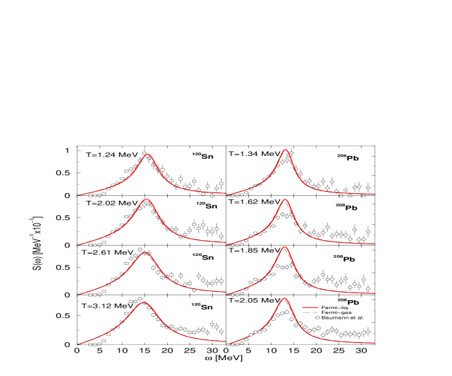
Figure 3.7: The IVGDR strength function in ¹²⁰Sn (LHS) and ²⁰⁸Pb (RHS) within the Fermi gas model (dashed lines) and Fermi liquid model (solid lines) at several temperatures compared with normalized data from Ref. [86].

The good overall agreement of the shape evolution with the experiment is again accompanied by only minor differences between the Fermi gas and the Fermi liquid model.

3.6 Higher order modes - surface modes

The existence of isoscalar giant dipole resonance (ISGDR) in nuclear matter is considered as a spurious mode in most text books since one associates with it a center of mass motion. The more surprising was the experimental justification of a giant resonance carrying the quantum numbers of a isoscalar and dipole mode [87, 76, 88]. Consequently one has to consider higher harmonics as explanation of such a mode [87, 89, 90]. Usually this mode is associated with a squeezing mode analogous to a sound wave [87, 76, 91, 88].

In this chapter we want to discuss the influence of surface effects on the ISGDR compression mode. We will show that even in the frame of the Fermi liquid model such modes can be understood. Moreover we claim that the surface effects are not negligible for reproducing the strength function. While we have already given a phenomenological approach to include surface effects we want to show now a straightforward possibility to include surface effects in the response function. Consequently we give first a short derivation of response function including surface effects. This will result in a new formula in the temperature-dependent extended Thomas-Fermi approximation [92].

The starting point is again the semi-classical Vlasov equation (2). Instead of using now a spatial homogeneous equilibrium as done so far we consider now explicitly the spatial dependence. Provided we know the response to the external potential without self-consistent mean field, which is described by the polarization function $\Pi$

$$\delta n({\bf x},t)=\int d{\bf x}^{\prime}\Pi({\bf x,x^{\prime}},t)U^{\rm ext}({\bf x^{\prime}},t),$$ (3.29)

the response including mean field, $\chi$, is given by

$$\chi({\bf x,x^{\prime}},t)=\Pi({\bf x,x^{\prime}},t)+\int d{\bf x}_{1}d{\bf x}_{2}\Pi({\bf x},{\bf x}_{1},t){\delta U^{\rm ind}({\bf x}_{1},t)\over\delta n({\bf x}_{2},t)}\chi({\bf x}_{2},{\bf x^{\prime}},t).$$ (3.30)

Therefore we concentrate first on the calculation of the polarization function $\Pi$ and linearize the Vlasov equation (2) according to $f({\bf p,R},t)=f_{0}({\bf p,R})+\delta f({\bf p,R},t)$ such that the induced density variation $\delta\rho({\bf R},t)=\int d{\bf p}\delta f/(2\pi\hbar)^{3}$ reads

$$\delta\rho({\bf x},\omega)=\int{d{\bf q}\over(2\pi\hbar)^{3}}{\rm e}^{i{\bf qx}}\int{d{\bf p}d{\bf x^{\prime}}\over(2\pi\hbar)^{6}}{\rm e}^{-i{\bf qx^{\prime}}}{{\bf\nabla}_{p}f_{0}({\bf p,x^{\prime}}){\bf\nabla}_{x^{\prime}}U^{\rm ext}({\bf x^{\prime}},t)\over i(\omega-{{\bf pq}\over m})}.$$

(3.31)

Here we have employed the Fourier transform of space and time coordinates of (2) to solve for $\delta f$ and inverse transform the momentum into the form (3.31). Comparing (3.31) with the definition of the polarization function (3.29) we extract with one partial integration

$$\Pi({\bf x,x^{\prime}},\omega)=-{\bf\nabla}_{x^{\prime}}\int{d{\bf p}d{\bf q}\over(2\pi\hbar)^{6}}{\rm e}^{i{\bf q}({\bf x-x^{\prime}})}{{\bf\nabla}_{p}f_{0}({\bf p,x^{\prime}})\over i(\omega-{{\bf pq}\over m})}.$$ (3.32)

With (3.32) and (3.30) we have given the polarization and response functions for a finite system.

In the following we are interested in the gradient expansion since we believe that the first order gradient terms will bear the information about surface effects. Therefore we change to the center of mass and difference coordinates ${\bf R}=({\bf x}_{1}+{\bf x}_{2})/2$, ${\bf r}={\bf x}_{1}-{\bf x}_{2}$ and retaining only first order gradients we get from (3.32) after Fourier transform of ${\bf r}$ into ${\bf q}$

$$\Pi({\bf R,q})=-\int{d{\bf p}\over(2\pi\hbar)^{3}}{{\bf q\nabla}_{p}f_{0}({\bf p,R})\over\omega-{{\bf pq}\over m}}+{i\over 2}{\bf\nabla}_{R}\int{d{\bf p}\over(2\pi\hbar)^{3}}\biggl{(}{{\bf\nabla}_{p}f_{0}({\bf p,R})\over\omega-{{\bf pq}\over m}}-{{\bf p}\over m}{{\bf q.\nabla}_{p}f_{0}({\bf p,R})\over(\omega-{{\bf pq}\over m})^{2}}\biggr{)}$$ (3.33)

$$= -\int{d{\bf p}\over(2\pi\hbar)^{3}}[{\bf q}-i{\bf\nabla}_{R}(1+{\omega\over 2}\partial_{\omega})]{{\bf\nabla}_{p}f_{0}({p^{2}\over 2m},{\bf R})\over\omega-{{\bf pq}\over m}}$$

where in the last equality we have assumed radial momentum dependence of the distribution function $f_{0}$. We recognize that besides the usual Lindhard polarization function as the first part of (3.33) we obtain a second part which is expressed by a gradient in space. The first part corresponds to the Thomas-Fermi result where we have to use the spatial dependence in the distribution functions and the second part represents the extended Thomas-Fermi approximation. So far we did not assume any special form of the distribution function. Therefore the expression (3.33) is also valid for any high temperature polarization of finite systems.

What remains to be shown is that the response function (3.30) does not contain additional gradients. This is easily confirmed by two equivalent formulations of (3.30), $\Pi^{-1}\chi=1+V\chi$ and $\chi\Pi^{-1}=1+\chi V$, which by adding yield the anticommutator

$$[\Pi^{-1},\chi]_{+}=2+[V,\chi]_{+}.$$ (3.34)

This anticommutator does not contain any gradients up to second order. Therefore we have [$V={\delta U^{\rm ind}/\delta n}$]

$$\chi({\bf R,q},\omega)={\Pi({\bf R,q},\omega)\over 1-V({\bf R,q},\omega)\Pi({\bf R,q},\omega)}+{\cal O}(\partial_{R}^{2}).$$ (3.35)

Equation (3.35) and (3.33) give the response and polarization functions of finite systems in first order gradient approximation.

Now we are ready to derive approximate formulae for spherical nuclei. In this case we can assume ${\bf q}||{\bf R}$ and we have

$$\Pi(R,{\bf q},\omega)=\Pi^{0}(R,{\bf q},\omega)-{i\over q}\partial_{R}\left[1+{\omega\over 2}\partial_{\omega}\right]\Pi^{0}(R,{\bf q},\omega)$$ (3.36)

where $\Pi_{0}$ is the usual Lindhard polarization with spatial dependent distributions (chemical potentials, density). We use now further approximations. In the case of giant resonances we are in the regime of small $q$ and ${\rm Im}\Pi^{0}\sim\omega$ such that

$$\left[1+{\omega\over 2}\partial_{\omega}\right]\Pi^{0}=i\frac{3}{2}{\rm Im}\Pi^{0}$$ (3.37)

since ${\rm Re}\Pi^{0}\sim 1-c^{2}q^{2}/\omega^{2}$. Within the local density approximation we know that the spatial dependence is due to the density $\rho(R)=\rho_{0}\Theta(R_{0}-R)$. Since we have for zero temperature ${\rm Im}\Pi^{0}\propto p_{f}(\rho)$ we evaluate

$$\partial_{R}{\rm Im}\Pi^{0}=-n_{0}\delta(R_{0}-R)\partial_{n}{\rm Im}\Pi^{0}=-\frac{1}{3}\delta(R_{0}-R){\rm Im}\Pi^{0}$$

(3.38)

where we assumed the density dependence carried only by the Fermi momentum. Now it is straightforward to average (3.36) over space with the help of (3.38)

$$\Pi({\bf q},\omega) = {3\over R_{0}^{3}}\int\limits_{0}^{R_{0}}dRR^{2}\Pi(R,{\bf q},\omega)$$ (3.39)

$$\approx \Pi^{0}({\bf q},\omega)+i{3\over qR_{0}}\left[1+{\omega\over 2}\partial_{\omega}\right]\frac{1}{3}\Pi^{0}({\bf q},\omega)$$

$$= \Pi^{0}+\Pi^{\rm surf}.$$

Consequently the surface contribution to the polarization function reads finally with (3.37)

$$\Pi^{\rm surf}({\bf q},\omega)=-{3\over 2qR_{0}}{\rm Im}\Pi^{0}({\bf q},\omega)$$ (3.40)

which is real. With (3.39), (3.40) and (3.35) we obtain now for the structure function

$$S(q,\omega)=\frac{1}{\pi}{{\rm Im}\Pi^{0}\over(1-V({\rm Re}\Pi^{0}+\Pi^{\rm surf}))^{2}+(V{\rm Im}\Pi^{0})^{2}}.$$ (3.41)

For small $q$ expansion we see that the pole of the structure function becomes renormalized similar to what is known from the Mie mode or surface plasmon mode [93, 94]

$$\omega^{2}={\omega_{0}^{2}\over 1-V\Pi^{\rm surf}}.$$ (3.42)

After establishing the structure function including surface contribution we specify the model for actual calculations. We choose as mean field parameterization a Skyrme force (3.17) following Vautherin and Brink [95] which leads to the isoscalar potential

$$V=U_{n}-U_{p}=\frac{3t_{0}}{4}+\frac{3t_{3}}{8}n_{0}$$ (3.43)

with $t_{0}=-983.4$ MeV fm³, $t_{3}=13106$ MeV fm⁶, $x_{0}=0.48$ at nuclear saturation density $n_{0}=0.16$ fm^-3 and the incompressibility of $K=318$ MeV. Further we employ again the Steinwedel-Jensen model [96] where the basic mode inside a sphere of radius $R_{0}$ is given by a wave vector

$$q_{sp}={\pi\over 2R_{0}}.$$ (3.44)

This would correspond to the first order isovector mode [97]. Since this mode is spurious we have to consider the next higher harmonics [98] which is

$$q_{isgdr}={\pi\over R_{0}}.$$ (3.45)

The polarization function with this second order mode contains still contributions from the spurious mode such that we have to subtract this part [89, 90]

$$\Pi^{0}_{\rm ISGDR}(\omega)=\Pi^{0}(q_{isgdr},\omega)-\Pi^{0}(q_{sp},\omega).$$ (3.46)

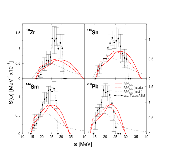
Figure 3.8: The experimental structure function (T=0) versus theoretical values. The bulk RPA result (solid lines) is compared with the extended Thomas Fermi approximation (surface corrections, dashed lines) and the inclusion of collisions (dot-dashed lines). The latter one should be of less importance due to symmetry of isoscalar mode. The data suggest this case and support surface contributions. Circles: Normalized data from Ref. [99]

In figure 3.8 we have plotted the experimental structure function together with different theoretical estimates according to (3.46) and (3.41). The inclusion of surface corrections (dashed lines) shifts the structure function towards the experimental values. The inclusion of collisions (dot-dashed lines), which should be wrong for isoscalar dipole mode due to cancellation of backscattering leads to really worse results. This supports indirectly that the mode is of isoscalar dipole type and surface dominated.

3.7 Simplified model for nuclear matter situation

The resulting wave vectors have very low values compared with the Fermi wave vector in the Steinwedel Jensen model. This allows us to expand the Mermin polarization function (3.12) with respect to small $qv_{c}/\omega$ ratios and $v_{c}$ the sound velocity. We obtain

$$\Pi_{a}^{\rm M}(\omega) = \frac{\rho_{a}(\mu_{a})}{m_{a}}{q^{2}\over\omega(\omega+{i/\tau_{a}})},$$ (3.47)

$$\rho_{a}(\mu_{a}) = 2\,\lambda_{a}^{-3}f_{3/2}(z_{a})\zeta_{corr}$$ (3.48)

where the thermal wave length is $\lambda_{a}^{2}=2\pi\hbar^{3}/(m_{a}T)$, $f_{3/2}$ the standard Fermi integral and $z_{a}={\rm e}^{\mu_{a}/T}$ the fugacity. The correction constant $\zeta_{corr}=1.22$ is introduced to fit the numerical solution of the dispersion relation (3.2) with the approximative expansion (3.47). With the help of this expansion the dispersion relation (3.11) takes the form

$$0 = \bigg{[}\omega\Big{(}\omega+\frac{i}{\tau_{n}}\Big{)}-c_{nn}^{2}q^{2}\bigg{]}\bigg{[}\omega\Big{(}\omega+\frac{i}{\tau_{p}}\Big{)}-c_{pp}^{2}q^{2}\bigg{]}$$ (3.49)

$$\!\!\!-\left[c_{np}^{2}+i{\tilde{c}_{np}^{2}\over(\omega+{i/\tau_{n}})\tau_{p}}\right]\left[c_{pn}^{2}+i{\tilde{c}_{pn}^{2}\over(\omega+{i/\tau_{p}})\tau_{n}}\right]q^{4}$$

with the partial sound velocities $c$ and $\tilde{c}$

$$c_{ab}^{2}=\alpha_{ab}\frac{\rho_{a}(\mu_{a})}{m_{a}},\qquad\tilde{c}_{ab}^{2}=\frac{T}{m_{a}}\frac{\frac{f_{3/2}(z_{a})}{f_{1/2}(z_{a})}-\frac{f_{3/2}(z_{b})}{f_{1/2}(z_{b})}}{\frac{\tau_{ab}}{\tau_{bb}}-\frac{\tau_{aa}}{\tau_{ba}}}.$$ (3.50)

The dispersion relation (3.11) with the dynamical relaxation times (3.16) is a polynomial of tenth (sixth) order corresponding to the inclusion of memory (in)dependent relaxation times. While most of these solutions will just lead to parasite solutions (${\rm Re}\,\omega\leq 0$) we will get two coupled modes, i.e. the isoscalar and isovector mode. Furthermore a third mode appears at extreme asymmetries and/or strong collisional coupling which we will describe in the next section.

3.8 New collective mode

Now we employ the potential (3.17) and assume different neutron and proton densities. In figure 3.9 we plot the isoscalar and isovector modes versus temperature for ${}^{48}Ca$ with a small asymmetry $\delta=0.2$ as well as for ${}^{60}Ca$ with an asymmetry $\delta=0.33$. The kinetic energy is linked to a temperature within the Fermi liquid model via Sommerfeld expansion

$${{\cal E}\over A}_{\rm kin} = \frac{3}{5}\epsilon_{f}\left[{(1+\delta)^{5/3}+(1-\delta)^{5/3}\over 2}\right.+\left.{5\over 12}\pi^{2}\left({T\over T_{f}}\right)^{2}{(1+\delta)^{1/3}+(1-\delta)^{1/3}\over 2}\right].$$ (3.51)

This connection between temperature and excitation energy is only valid for a continuous Fermi liquid model. For small nuclei, the concept of temperature is questionable. Some improvement can be obtained by the definition of temperature via the logarithmic derivative of the density of states [100]

$$T^{-1}=\frac{1}{\rho}{\partial\rho\over\partial E_{\rm ex}}=-\frac{5}{4}E_{\rm ex}^{-1}+\pi({A\over 4\epsilon_{f}E_{\rm ex}})^{1/2}$$ (3.52)

which provides $E_{\rm ex}\approx\frac{1}{4}(E/A)$ in comparison with (3.51) for small temperatures and small nuclei. We use this temperature to demonstrate possible collective bulk features in an exploratory sense. Of course, the surface energy and shell effects cannot be neglected for realistic calculations of small nuclei.

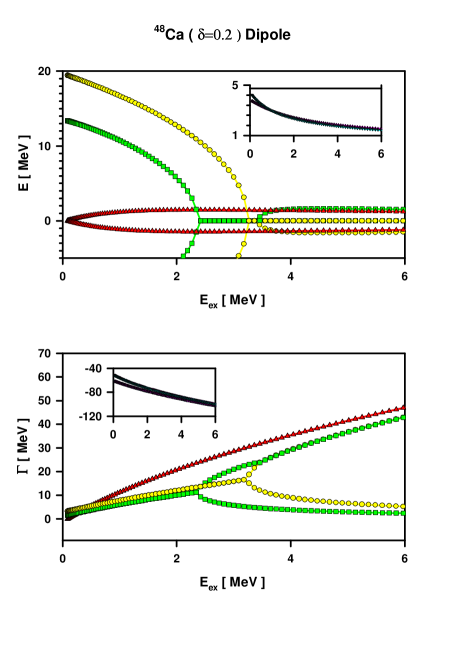
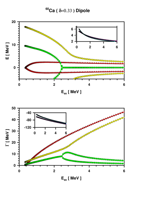
Figure 3.9: The energy and damping of the IVGDR and ISGDR of ${}^{48}Ca$ (left) and ${}^{60}Ca$ (right) vs excitation energy. Besides the isovector modes (circles) and the isoscalar modes (squares) a soft third mode appears (triangles).

With increasing temperature the isovector and isoscalar energies decrease and vanish at a certain temperature. At these temperatures the damping becomes twofold because the damping of the spurious mode with negative energy becomes different from the physical mode. We can consider this behavior of damping as a phase transition of isospin demixture. At the same time a very soft mode appears due to collisional coupling which is only present in asymmetric matter [18]. This mode is more pronounced in the next figure 3.9 for ${}^{60}Ca$ with an asymmetry of $\delta=0.33$.

We see that the isovector mode does not disappear but turns over into a flat decrease with increasing temperature. This behaviour is coupled with the pronounced soft mode. In comparison with the more symmetric ${}^{48}Ca$ we see a different behavior of the damping where the isoscalar mode vanishes. Also the isovector mode appears unique and not two-fold. Now a clear transition of damping behavior for the isovector mode is recognizable which can be considered as a transition from zero to first sound damping.

Besides the standard isovector and isoscalar modes we observe a build up of a very soft mode with a centroid energy around $1$ MeV. This mode appears due to the collisional coupling $\bar{c}_{ab}^{2}$ of (3.50). When we turn off the relaxation times, i.e. the collision integral, this mode is vanishing as well as in symmetric nuclear matter, see discussion after (3.13). It shows that this mode appears due to collisional coupling of isovector and isoscalar modes. The corresponding damping of the crossed mode is continuously increasing with temperature.

One may argue whether this third mode can really appear in the system. A simple consideration may convince us about the possible existence of such mode. Let us assume a coupled set of two type of harmonic oscillators (neutrons and protons) interacting between the same sort of particles with strength $k_{n}$ and $k_{p}$, respectively and between different sorts with $k_{np}$. Let us choose for simplicity only two neutrons and two protons. Then we obtain the coupled system of harmonic oscillators with frequencies $\omega_{n}^{2}=k_{n}/m$, $\omega_{p}^{2}=k_{p}/m$ and $\omega_{np}^{2}=k_{np}/m$. The solution yields three basic modes in the system, i.e. $\omega^{2}=2(\omega_{n}^{2}+\omega_{np}^{2}),4\omega_{np}^{2},2(\omega_{p}^{2}+\omega_{np}^{2})$. If we neglect the different coupling between neutrons and protons $\omega_{np}$ we only obtain two modes analogously to isovector and isoscalar ones. We see that the coupling between neutrons and protons can lead to the appearance of a third mode.

Let us now compare the found new mode with the experimental evidence. There are some hints for a soft mode in ${}^{11}Be$ [101]. The authors have observed a low lying structure at around $6$ MeV excitation energy with a damping of around $1$ MeV which has not been reproduced yet even within refined coupled channel calculations [102]. A standard explanation would give as the origin a weakly-bound single particle neutron orbital. The observed broad structure at $6$ MeV might be explained alternatively as the presented new coupled mode. The centroid energy as well as damping width at least seem to suggest this interpretation.

Chapter 4 Nonlinear effects beyond linear response

While most of the theoretical treatments of oscillations rely on the linear response method or RPA methods, large amplitude oscillations require methods beyond. In particular the question of the appearance of chaos has recently been investigated [44, 45, 46]. The hypothesis was established that the octupole mode is over-damped due to negative curved surface and consequently additional chaotic damping [47, 48, 49]. Here we want to discuss in which conditions one might observe octupole modes at least in Vlasov - simulation of giant resonances. We will consider different initial conditions of isoscalar giant resonances and will demonstrate that the appearance of octupole modes is dependent on the initial configuration which in turn demonstrates the nonlinear behavior beyond linear response.

As a first initial condition we use the ground state distribution of coordinates while the momentum distribution is deformed anisotropically. We have modified the momenta in a way which corresponds to a giant octupole mode. The local densities and currents remain the same as in ground state. Figure 4.1 shows that at start time $t=0$ there is a pure giant octupole, which is damped out and a quadrupole resonance develops instead. The monopole and dipole amplitudes which should remain constant document the stability of simulation. In agreement with the already mentioned hypothesis, the octupole mode is over-damped. The figure shows the nonlinear behavior of mode coupling. Within the linear response the damping rate is expected to be independent of initial conditions. We choose now other initial conditions to show that the result is very much dependent on initial conditions. Therefore we split the nucleus in two parts of mass ratio 3:7 in accordance with the symmetry of the octupole oscillation and accelerate both pieces towards each other. Experimentally this might be realized as a central collision of two nuclei with corresponding masses.

Figure 4.1: The picture shows the time evolution of multipole moments $\sqrt{\frac{2l+1}{4\pi}}a_{l0}(t),l=0,1,2,3$ of mass density concerning to normalization, dipole, quadrupole and octupole oscillation. Excitation is due to modification in momentum space only.

In figure 4.2 a clear quadrupole resonance appears and also a smaller octupole resonance can be seen. Both are damped out. Consequently there is no evidence for an over-damped octupole mode in this case.

In order to understand the different initializations, we split the kinetic energy into a thermal part and a collective part according to $\langle{\bf p}^{2}\rangle=\left\langle({\bf p}-\langle{\bf p}\rangle)^{2}\right\rangle+\langle{\bf p}\rangle^{2}$. We analyze the time development of the total collective energy in the system

$$E_{coll}(t) = \frac{h^{2}}{2m}\int d{\bf r}\varrho({\bf r})\langle{\bf p}\rangle^{2}({\bf r},t)$$ (4.1)

with the mean current

$$\langle{\bf p}\rangle({\bf r},t) = \frac{1}{\varrho({\bf r})}\int\frac{d{\bf p}}{(2\pi)^{3}}\;{\bf p}\;f({\bf p,r},t)$$ (4.2)

and the density

$$\varrho({\bf r},t) = \int\frac{d{\bf p}}{(2\pi)^{3}}\;f({\bf p,r},t)\;.$$ (4.3)

Figure 4.2: This picture shows the time evolution of multipole moments $\sqrt{\frac{2l+1}{4\pi}}a_{l0}(t),l=0,1,2,3$ of mass density. Excitation is due to asymmetric splitting (0.3 to 0.7) of the nucleus in two pieces using a plane in coordinate space. Then both pieces are accelerated towards each other.

In figure 4.3 the development of collective energy can be seen. There is a background of about 50 MeV due to fixed correlations caused by finite width of pseudo-particles as one can see from the following estimation. Using (3.7) and (3.39) in (4.1) one obtains

$$E_{coll} \approx {\textstyle\frac{1}{\varrho_{0}}}\sum_{i=1}^{AN}\sum_{j=1}^{AN}{\textstyle\frac{1}{N^{2}}}p_{i}p_{j}\int drf_{S}(r-r_{i}(t),\sigma_{r})f_{s}(r-r_{j}(t),\sigma_{r})$$ (4.4)

$$\approx {\textstyle\frac{1}{\varrho_{0}}}\sum_{i=1}^{AN}\sum_{j=1}^{AN}{\textstyle\frac{1}{N^{2}}}p_{i}p_{j}f_{S}(r_{i}(t)-r_{j}(t),\sqrt{2}\sigma_{r})$$

$$\geq {\textstyle\frac{1}{\varrho_{0}N}\frac{1}{(\sqrt{2\pi}\sqrt{2}\sigma_{r})^{3}}}\sum_{i=1}^{AN}{\textstyle\frac{1}{N}}p_{i}.$$

For simulation parameters of ${}^{208}Pb$, $\rho_{0}=0.162\;{\rm fm}^{-3}$, $N=75$, $\sigma_{r}=0.53\;{\rm fm}$, we obtain a basic collective energy of ${54\rm MeV}$. Using more test-particles would diminish this level.

The solid line corresponding to figure 4.1 shows no initial collective energy. The exclusive initial excitation in momentum space without correlation in the spatial domain leads to zero initial collective energy. These correlations are forming during time evolution. Of course, there is no center of mass motion, otherwise we would see just the mean streaming velocity.

This situation is changed if we use the second preparation with simple momentum–space–correlations. The long dashed line in figure 4.3 shows initial collective correlations corresponding to figure 4.2. Since we can deposit enough collective energy in this case, we observe a clear octupole motion.

Figure 4.3: The time evolution of collective energy. The solid line corresponds to the excitation scheme of figure 4.1 and the long dashed line corresponds to the figure 4.2, respectively. While the first starts without collective energy, the second one starts with maximal collective energy.

In order to compare with [48] we calculate the adiabaticity index $\eta$ defined in [48] as the ratio of maximum radial surface velocity to the maximum particle speed. A smaller ratio denotes a more adiabatic shape changes in relation to the particle speed. In analogy we define such index as a ratio

$$\eta = \frac{\frac{\partial}{\partial t}\sqrt{<r^{2}>(\vartheta)}}{v_{F}}$$ (4.5)

of the root mean square radius speed in forward direction (opening angle $\vartheta$) and the Fermi velocity. With opening angle 0.4 rad we obtain a maximum $\eta=0.12$ for figure 4.1 and $\eta=0.30$ for figure 4.2. This shows that we are essentially still in the adiabatic regime described in [48].

The nonlinear behavior described so far already documents that we are in a regime of large amplitude oscillations where linear response fails. The corresponding radius elongation in coordinate space varies about 10 %.

Chapter 5 Summary

We have investigated the giant resonance oscillations by solving the collision-less Vlasov equation as well as by linear response theory.

With the help of numerical solution of the Vlasov equation we could reproduce the mass dependence of energy with one fixed parameter of test-particle width for both giant monopole and giant dipole modes. A multipole analysis was performed which has allowed us to characterize the corresponding excitation. It was shown, that the asymmetry influences the collective behavior. With increasing asymmetry the energy decreases while the damping increases. The damping due to finite systems amount to $2$MeV almost constant for all mass numbers which underestimates the experimental values considerably. This motivates to search for additional damping mechanism which was found to be due to the collisional correlations.

The linear response can be used in a simplified liquid drop model to describe the giant resonances in asymmetric matter. We find that the collisional contribution as well as surface contributions are both important to reproduce the experimental damping of giant dipole resonances. While for ground state resonances it is sufficient to add the damping of finite size effects from simulation with the collisional contribution from linear response theory, for the temperature behavior we have needed also the deformation of the surface. The combined model between surface and collisional contribution, weighted properly due to their collision frequencies, is able to reproduce the experimental damping curve with temperature as well as the structure function. A higher order mode like the recently measured ISGDR mode has been described within this simple linear response model.

We have observed that due to correlational coupling there can exist a new mode which appears besides isovector and isoscalar modes in asymmetric nuclear matter due to collisions. We suggest that this mode may be possible to observe as a soft collective excitation in asymmetric systems. The transition from zero sound damping to first sound damping behavior should become possible to observe for isovector modes since they do not vanish at this transition temperature like in symmetric matter. At a certain critical temperature the collective isoscalar mode vanishes and the damping becomes two-fold. This can be considered as a phase transition of demixture.

On the example of octupole resonances in finite nuclei the dependency on the initial configuration is demonstrated. The appearance of an octupole mode was shown by correlating the spatial and momentum initial excitation. It is possible to excite an octupole mode with sufficient collective energy deposited initially. We suggest that isoscalar giant octupole resonances should be possible to observe in nuclear collisions of mass ratio about 3:7 corresponding to octupole symmetry. This effect illustrates a mode beyond linear response.

5.1 Acknowledgment

The authors are obliged to M. Vogt who has contributed the calculation of the Lyapunov exponent. M. DiToro is thanked for numerous discussions and the LNS Catania where part of this work was done for hospitality. Valuable hints and comments by J. D. Frankland (GANIL) are also gratefully acknowledged.

Appendix A Derivation of non-Markovian relaxation time

Here we shortly sketch the derivation of the damping of a collective mode within a Fermi gas and a Fermi liquid model. We will show that we get the latter one from the Fermi gas model with an additional contribution from the quasi-particles.

We start with the Fermi gas where the dispersion relation between momentum and energy is given by $\epsilon=p^{2}/2m$ and will show later what has to be changed for a Fermi liquid where $\epsilon$ is a solution of the quasiparticle dispersion relation. We will see that the contributions from the quasi-particles alone leads to the Landau formula of zero sound damping [103, 104]

$$\gamma\propto\left[1+\left({\Omega\over 2\pi T}\right)^{2}\right].$$ (A.1)

Our considerations use conveniently the Levinson equation for the reduced density matrix $f$ which is valid at short time processes compared to inverse Fermi energy $\hbar/\epsilon_{f}$ and which collisional side has the form:

$$I_{1}(t)={2g\over\hbar^{2}}\int\limits_{0}^{\infty}d\tau\int{d{\bf p}_{2}d{\bf p}_{3}d{\bf p}_{4}\over(2\pi\hbar)^{6}}|T|^{2}\cos{\left(\int\limits_{t}^{t-\tau}\Delta\epsilon(\tau)d\tau/\hbar\right)}\delta(\Delta{\bf p})\left({\bar{f}_{1}}{\bar{f}_{2}}f_{3}f_{4}-f_{1}f_{2}{\bar{f}_{3}}{\bar{f}_{4}}\right)_{t-\tau}$$ (A.2)

where ${\bar{f}}=1-f$, $\Delta p=p_{1}+p_{2}-p_{3}-p_{4}$ etc., g is the spin-isospin degeneracy and the transition probability is given by the scattering $T$-matrix. In case that the quasiparticle energies $\epsilon(t)$ become time independent like in the Fermi gas model, the integral in the $cos$ function reduces to the familiar expression $\Delta\epsilon\tau$. We linearize this collision integral with respect to an external disturbance according to

$$f=n+\delta f$$ (A.3)

where n is the equilibrium distribution. Clearly two contributions have to be distinguished, the one from the quasiparticle energy and the one from occupation factors [6]. First we concentrate on the Fermi gas model where we have only the contribution of the occupation factors and will later add the contribution of the quasiparticle energies for Fermi liquid model. We obtain after Fourier transform of the time

$$\delta I_{1} = \Big{\langle}\frac{\hbar}{2}\left[\delta_{+}(\Delta\epsilon+\Omega)+\delta_{-}(\Delta\epsilon-\Omega)\right]\left(\delta F_{1}+\delta F_{2}-\delta F_{3}-\delta F_{4}\right)(\Omega)\Big{\rangle}.$$ (A.4)

Here we use the abbreviation

$$\langle...\rangle = {2g\over\hbar^{2}}\int{d{\bf p}_{2}d{\bf p}_{3}d{\bf p}_{4}\over(2\pi\hbar)^{6}}|T|^{2}\delta(\Delta p)...={m^{3}g\over\hbar^{2}(2\pi\hbar)^{6}}\int d\epsilon_{2}d\epsilon_{3}d\epsilon_{4}\int{d\phi\sin\theta d\theta d\phi_{2}\over\cos(\theta/2)}|T|^{2}...$$

where the last line appears from standard integration techniques at low temperatures. Further abbreviations are

$$\delta_{\pm}(x) = \pi\delta(x)\pm i{{\cal P}\over x}\approx\pi\delta(x)$$

$$\delta F_{1} = -\delta f_{1}({\bar{n}_{2}}n_{3}n_{4}+n_{2}{\bar{n}_{3}}{\bar{n}_{4}}).$$ (A.6)

The approximation used in the first line consists in the neglect of the off-shell contribution from memory effects. This is consistent with the used integration technique (LABEL:int). This terms would lead to divergences which has to be cut off [53].

Neglecting the backscattering terms $\delta F_{2/3/4}$ we obtain from (A.4) a relaxation time approximations with the relaxation time

$${1\over\tau(\epsilon_{1})}={3\over 4\pi^{2}\tau_{0}}\int\limits_{-\lambda}^{\infty}dx_{2}dx_{3}dx_{4}\left[\delta(\Delta x+\omega)+\delta(\Delta x-\omega)\right]({\bar{n}_{2}}n_{3}n_{4}+n_{2}{\bar{n}_{3}}{\bar{n}_{4}})$$ (A.7)

with $\omega=\Omega/T$, $x=(\epsilon-\mu)/T$, $\lambda=\mu/T$ and the time

$${1\over\tau_{0}}={2gmT^{2}\over 3\hbar^{3}}\sigma.$$ (A.8)

Here we have used the definition of cross section $|T|^{2}=(4\pi\hbar^{2}/m)^{2}d\sigma/d\Omega$ and have assumed a constant cross section $\sigma$. To calculate (A.7) one needs the standard integrals for large ratios of chemical potentials $\mu$ to temperature $\lambda=\mu/T$

$$\int\limits_{-\lambda}^{\infty}dx_{2}dx_{3}dx_{4}n_{2}{\bar{n}_{3}}{\bar{n}_{4}}\delta(\Delta x\pm\omega)=\frac{1}{2}{\bar{n}_{1}}(x_{1}\pm\omega)\left[\pi^{2}+(x_{1}\pm\omega)^{2}\right]$$ (A.9)

to obtain

$${1\over\tau(\epsilon_{1})}={3\over 8\pi^{2}\tau_{0}}\left[2\pi^{2}+(x_{1}+\omega)^{2}+(x_{1}-\omega)^{2}\right].$$ (A.10)

Further we employ a thermal averaging in order to obtain the mean relaxation time finally

$${1\over\tau_{\rm gas}}=\int\limits_{-\lambda}^{\infty}dx_{1}n_{1}{\bar{n}_{1}}{1\over\tau(\epsilon_{1})}={1\over\tau_{0}}\left[1+3\left({\omega\over 2\pi}\right)^{2}\right].$$ (A.11)

If we do not use the thermal averaging but take (A.10) at the Fermi energy $\epsilon_{1}=\epsilon_{f}$ we will obtain

$${1\over\tau(\epsilon_{f})}={1\over\tau_{0}}\left[\frac{3}{4}+3\left({\omega\over 2\pi}\right)^{2}\right].$$ (A.12)

We see that both results disagree with the Landau result of quasiparticle damping (A.1) by factors of 3 at different places [6, 71, 105, 106]. We have point out that the result at fixed Fermi energy will lead to unphysical results for the Fermi liquid case. Therefore we consider the thermal averaged result as the physical one.

We now turn to the Fermi liquid model and replace the free dispersion $\epsilon=p^{2}/2m$ by the quasiparticle energy $\epsilon_{p}$. Than the variation of the collision integral gives an additional term which comes from the time dependence of the quasiparticle energy on the $\cos$-term of (A.2). We have instead of the sum of two complex conjugate exponentials in (A.2) an additional contribution from the linearization of the exponential

$$\delta\exp{\left(i\Delta\int\limits_{t}^{t-\tau}d{\bar{t}}\epsilon({\bar{t}})\right)} = {\rm e}^{-i\Delta\epsilon\tau}\left(1-i\Delta\int\limits_{t}^{t-\tau}d{\bar{t}}[\epsilon({\bar{t}})-\epsilon]\right)-{\rm e}^{-i\Delta\epsilon\tau}$$ (A.13)

$$= {iT\over\hbar}{\rm e}^{-i\Delta\epsilon\tau/\hbar}\Delta\int\limits_{t}^{t-\tau}d{\bar{t}}{\delta f({\bar{t}})\over n{\bar{n}}}.$$

In the last line we have replaced the variation in the quasiparticle energy $\epsilon(t)-\epsilon$ by the variation in the distribution function $\delta f$ due to the identity [104]

$$\delta f(t) = f(t)-n(\epsilon)=f(t)-n(\epsilon(t))-[n(\epsilon)-n(\epsilon(t))]$$ (A.14)

$$\approx -n^{\prime}(\epsilon(t)-\epsilon)={n{\bar{n}}\over T}\left[\epsilon(t)-\epsilon\right]$$

where we assumed within the quasiparticle picture that $f(t)=n(\epsilon(t))$. This leads now to an additional part in the relaxation time which we write analogously to (A.4)

$${1\over\tau_{c}(\epsilon_{1})} = \left\langle\frac{\hbar}{2}{\delta_{+}(\Delta\epsilon-\Omega)-\delta_{+}(\Delta\epsilon+\Omega)\over\Omega}{{\bar{n}_{1}}{\bar{n}_{2}}n_{3}n_{4}-n_{1}n_{2}{\bar{n}_{3}}{\bar{n}_{4}}\over n_{1}{\bar{n}_{1}}}\right\rangle.$$ (A.15)

Using again (A.9) we obtain

$${1\over\tau_{c}(\epsilon_{1})}={-3\over 4\pi^{2}\tau_{0}}\Bigg{\{}\frac{{\bar{n}}(x_{1}+\omega)\left[\pi^{2}+(x_{1}+\omega)^{2}\right]}{2\omega({\rm e}^{-\omega}-1)}+\,[\omega\leftrightarrow-\omega]\Bigg{\}}$$ (A.16)

and get after thermal averaging (A.11)

$${1\over\tau_{c}}={1\over\tau_{0}}\left[1+\left({\omega\over 2\pi}\right)^{2}\right].$$ (A.17)

Taking instead of thermal averaging the value at Fermi energy $(\epsilon_{1}=\epsilon_{f})$ in (A.16) we find

$${1\over\tau_{c}(\epsilon_{f})}={3(\pi^{2}+\omega^{2})\over 2\pi^{2}\tau_{0}\omega}{{\rm e}^{\omega}-1\over{\rm e}^{\omega}+1}.$$ (A.18)

Here we like to point out that the Landau result (A.1) appears in (A.17) (see also in Ref. [71, 107, 19, 105, 106]).

Adding now (A.11) and (A.17) we obtain a final relaxation time for the Fermi liquid model

$${1\over\tau_{\rm liq}}={2\over\tau_{0}}\left[1+2\left({\omega\over 2\pi}\right)^{2}\right].$$ (A.19)

which is the main result in this paper. It contains the typical Landau result of zero sound (A.1) except the factor 2 in front of the frequencies. Comparing (A.19) with the Fermi gas model (A.11) we see that in the limit of vanishing temperature the Fermi liquid value is lower with $\propto 2\Omega^{2}$ compared to the Fermi gas $\propto 3\Omega^{2}$. Further for vanishing frequencies (neglect of memory effects) the Fermi liquid model leads to twice the relaxation rate than the Fermi gas model. The coefficient of temperature increase is than twice larger for the Fermi liquid than for the Fermi gas. If we consider the relaxation times at Fermi energy (no thermal averaging) (A.12) and (A.18) we find the same results as above in the limit of vanishing frequencies. For vanishing temperature only the Fermi gas (A.12) coincides with the result of (A.11) $\propto 3\Omega^{2}$. Expression (A.18) goes to zero for $T=0$ and underlines the necessity to thermal average the value.

Bibliography

- [1] W. Bothe and W. Gentner, Zeit. f. Physik 106, 236 (1937).
- [2] G. F. Bertsch, P. F. Bortignon, and R. A. Broglia, Rev. of Mod. Phys. 55, 287 (1983).
- [3] J. Bacelar, M. Harakeh, and O. Scholten, Nucl. Phys. A 599, 1 (1996), proceedings of the Groningen conference on giant resonances.
- [4] in Topical Conference on Giant Resonances Varenna, No. 3 in Nucl. Phys. A, edited by A. Bracco and P. Bortignon (Elsevier, North Holland, 1998), .
- [5] in Selected Topics in Nuclear Collective Excitatons, NUCOLEX99, Vol. 23 of Riken Rev., edited by N. D. Dang, U. Garg, and S. Yamaji (RIKEN, Hirosawa, Wako, Saitama, 1999), .
- [6] U. Fuhrmann, K. Morawetz, and R. Walke, Phys. Rev. C. 58, 1473 (1998).
- [7] F. Catara, E. G. Lanza, M. A. Nagarajan, and A. Vitturi, Nucl. Phys. A 624, 449 (1996).
- [8] S. Kamerdzhiev, Yad. Fiz. 9, 324 (1969).
- [9] H. Sagawa and G. F. Bertsch, Phys. Lett. B 5, 138 (1984).
- [10] V. Abrosimov, M. DiToro, and A. Smerzi, Z. Phys. A 347, 161 (1994).
- [11] V. M. Kolomietz, V. A. Pluiko, and S. Shlomo, Phys. Rev. C 52, 2480 (1995).
- [12] V. Kolomietz, V. Plujko, and S. Shlomo, Phys. Rev. C 54, 3014 (1996).
- [13] V. Kondratyev and M. Di Toro, Phys. Rev. C 53, 2176 (1996).
- [14] E. Hernández, J. Navarro, A.Polls, and J. Ventura, Nucl. Phys. A597, 1 (1996).
- [15] M. DiToro, V. Kolomietz, and A. Larionov, in Proceedings of the Dubna Conference on Heavy Ions, Dubna, 1997 (unpublished).
- [16] V. Kolomietz, A. Larionov, and M. DiToro, Nucl. Phys. A613, 1 (1997).
- [17] V. M. Kolomietz, S. V. Lukyanov, V. A. Plujko, and S. Shlomo, Phys. Rev. C 58, 198 (1998).
- [18] K. Morawetz, R. Walke, and U. Fuhrmann, Phys. Rev. C 57, R 2813 (1998).
- [19] S. Ayik, O. Yilmaz, A. Golkalp, and P. Schuck, Phys. Rev. C 58, 1594 (1998).
- [20] G. Gervais, M. Thoennessen, and W. E. Ormand, Phys. Rev. C, 1998.
- [21] S. Shlomo and G. F. Bertsch, Nucl. Phys. A243, 507 (1975).
- [22] H. Esbensen and G. F. Bertsch, Phys. Rev. C 28, 355 (1983).
- [23] H. Esbensen and G. F. Bertsch, Ann. Phys. 157, 255 (1984).
- [24] P. F. Bortignon, A. Bracco, D. Brink, and R. A. Broglia, Phys. Rev. Lett. 67, 3360 (1991).
- [25] W. E. Ormand, P. F. Bortignon, and R. A. Broglia, Phys. Rev. Lett. 77, 607 (1996).
- [26] S. Kamerdzhiev, J. Speth, and G. Tertychny, Nucl. Phys. A624, 328 (1997).
- [27] W. E. Ormand, P. F. Bortignon, R. A. Broglia, and A. Bracco, Nucl. Phys A614, 217 (1997).
- [28] S. Kamerdzhiev, R. J. Liotta, E. Litvinova, and V. Tselyaev, Phys. Rev. C 58, 172 (1998).
- [29] J. Kvasil, N. L. Iudice, V. O. Nesterenko, and M. Kopal, Phys. Rev. C 58, 209 (1998).
- [30] Y. Alhassid and B. Bush, Phys. Rev. Lett. 63, 2452 (1989).
- [31] W. E. Ormand et al., Phys. Rev. Lett. 64, 2254 (1990).
- [32] W. E. Ormand et al., Phys. Rev. Lett. 69, 2905 (1992).
- [33] B. Lauritzen, P. F. Bortignon, R. A. Broglia, and V. G. Zelevinsky, Phys. Rev. Lett. 74, 5190 (1995).
- [34] A. Bracco et al., Phys. Rev. Lett. 74, 3748 (1995).
- [35] S. Leoni, T. Døssing, and B. Herskind, Phys. Rev. Lett. 76, 4484 (1996).
- [36] M. DiToro, V. Kolomietz, and A. Larionov, Phys. Rev. C 59, 3099 (1999).
- [37] D. Lecroix, P. Chomaz, and S. Ayik, Phys. Rev. C 58, 2154 (1998).
- [38] M. Colonna et al., Phys. Lett. B 307, 293 (1993).
- [39] V. Baran et al., Nucl. Phys. A599, 29 (1996).
- [40] R. Walke and K. Morawetz, Phys. Rev. C. 60, 17301 (1999).
- [41] V. Špička, P. Lipavský, and K. Morawetz, Phys. Lett. A 240, 160 (1998).
- [42] K. Morawetz et al., Phys. Rev. Lett. 82, 3767 (1999).
- [43] D. Brink, A. Dellafiore, and M. DiToro, Nucl. Phys. A 456, 205 (1986).
- [44] W. Bauer, D. McGrew, V. Zeletvinsky, and P. Schuck, Phys. Rev. Lett. 72, 3771 (1994).
- [45] G.F.Burgio, M.Baldo, A.Rapisarda, and P. Schuck, Phys.Rev C 52, 2475 (1995).
- [46] K. Morawetz, Phys. Rev. C 55, R 1015 (1997).
- [47] C. Jarzynski and W. Swiatecki, Nucl. Phys. A 552, 1 (1993).
- [48] J. Blocki, J.-J. Shi, and W. Swiatecki, Nucl. Phys. A 554, 387 (1993).
- [49] J. Blocki, J. Skalski, and W. Swiatecki, Nucl. Phys. A 816, 1 (1997).
- [50] G. F. Bertsch and S. D. Gupta, Phys. Rep. 160, 189 (1988).
- [51] M. Colonna, M. D. Toro, and A. Guarnera, Nucl. Phys. A 589, 160 (1995).
- [52] K. Morawetz, Phys. Lett. A 199, 241 (1995).
- [53] K. Morawetz and H. Koehler, Eur. Phys. J. A 4, 291 (1999).
- [54] C. Wong, Phys. Rev. C 25, 1460 (1982).
- [55] M. Colonna et al., Phys. Rev. C 47, 1395 (1993).
- [56] K. Morawetz and R. Walke, Europ. Phys. J. A (1998), sub. nucl-th/9807045.
- [57] J. Blaizot, Phys. Rep. 64, 171 (1980).
- [58] C. Garcia, J. Navarro, V. Nguyen, and L. Salcedo, Ann. Phys. (N.Y.) 214, 293 (1992).
- [59] F. Braghin, D. Vautherin, and A. Abada, Phys. Rev. C 52, 2504 (1995).
- [60] H. Heiselberg, C. J. Pethick, and D. G. Ravenhall, Ann. Phys. 223, 37 (1993).
- [61] N. Mermin, Phys. Rev. B 1, 2362 (1970).
- [62] D. Kiderlen and H. Hofmann, Phys. Lett. B 332, 8 (1994).
- [63] G. Röpke and A. Wierling, Phys. Rev. E 57, 7075 (1998).
- [64] K. Morawetz and U. Fuhrmann, Phys. Rev. E 61, (2000).
- [65] P. Haensel, Nucl. Phys. A301, 53 (1978).
- [66] E. Hernández, J. Navarro, and A.Polls, Phys. Lett. B 413, 1 (1997).
- [67] M. Colonna, M. D. Toro, , and A. Larionov, Phys. Lett. B 428, 1 (1998).
- [68] F. Braghin, Phys. Lett. B 446, 1 (1999).
- [69] T. H. R. Skyrme, Phil. Mag. 1, 1043 (1956).
- [70] T. H. R. Skyrme, Nucl. Phys. 9, 615 (1959).
- [71] S. Ayik and D. Boilley, Phys. Lett. B 276, 263 (1992), errata ibd. 284 (1992) 482.
- [72] K. Morawetz, M. DiToro, and L. Münchow, Phys. Rev C. 54, 833 (1996).
- [73] N. D. Mermin, Phys. Rev. B 1, 2362 (1970).
- [74] V. Baran and et. al., Nucl. Phys. A632, 287 (1998).
- [75] H. Steinwedel and J. Jensen, Z. f. Naturforschung 5, 413 (1950).
- [76] B. F. Davis and et. al., Phys. Rev. Lett. 79, 609 (1997).
- [77] D. Vautherin and D. M. Brink, Phys. Rev. C 5, 626 (1972).
- [78] F. Braghin and D. Vautherin, Phys. Lett. B 333, 289 (1994).
- [79] S. Dietrich and B. Berman, Nucl. Data Tabl. 38, 199 (1988).
- [80] E. Ramakrishnan et al., Phys. Rev. Lett. 76, 2025 (1996).
- [81] E. Ramakrishnan et al., Nucl. Phys. A549, 49 (1996).
- [82] K. Morawetz et al., Phys. Rev. C. 60, 54601 (1999).
- [83] K. Morawetz, Phys. Rev. E. (2000), in press physics/9810046.
- [84] P. Ring and P. Schuck, The Nuclear Many-Body Problem (Springer-Verlag, New York, 1980).
- [85] W. Greiner and J. Maruhn, Nuclear Models (Springer-Verlag, Berlin et.al, 1996).
- [86] T. Baumann and et. al., Nucl. Phys. A635, 428 (1998).
- [87] M. Harakeh and A. E. L. Dieperink, Phys. Rev. C 23, 2329 (1981).
- [88] U. Garg, in Selected Topics in Nuclear Collective Excitatons, NUCOLEX99, Vol. 23 of Riken Rev., edited by N. D. Dang, U. Garg, and S. Yamaji (RIKEN, Hirosawa, Wako, Saitama, 1999), p. 65.
- [89] T. J. Deal, Nucl. Phys. A 217, 210 (1973).
- [90] I. Hamamoto, H. Sagawa, and X. Zhang, Phys. Rev. C. 57, R1064 (1998).
- [91] N. V. Giai and N. Sagawa, Nucl. Phys. A 371, 1 (1981).
- [92] P. Ring and P. Schuck, The Nuclear Many Body Problem (Springer, Heidelberg, 1980).
- [93] G. F. Bertsch and R. A. Broglia, Oscillations in finite Quantum Systems (Cambridge University Press, Cambridge, 1994).
- [94] U. Kreibig and M. Vollmer, Optical Properties of Metal Cluster (Springer-Verlag, Berlin, 1995).
- [95] D. Vautherin and D. Brink, Phys. Rev. C 5, 626 (1972).
- [96] H. Steinwedel and J. Jensen, Z. Naturforsch. 5, 413 (1950).
- [97] F. Braghin and D. Vautherin, Phys. Lett. B 333, 289 (1994).
- [98] K. Morawetz, U. Fuhrmann, and R. Walke, Nucl. Phys. A 649, 348 (1999).
- [99] U. Garg, private communication.
- [100] A. Bohr and B. R. Mottelson, Nuclear Structure (W. A. Benjamin, Inc., New York, 1969).
- [101] F. Cappuzzello and et. al., in Proceedings of the workshop on Large scale collective motion of atomic nuclei, Brolo 1996, edited by G. Giardina (World Scientific, Singapore, 1996), p. 88.
- [102] H. Esbensen, B. A. Brown, and H. Sagawa, Phys. Rev. C. 51, 1274 (1995).
- [103] A. A. Abrikosov and I. M. Khalatnikov, Rep. Prog. Phys. 22, 329 (1959).
- [104] E. Lifschitz and L. P. Pitaevsky, in Physical Kinetics, edited by E. Lifschitz (Akademie Verlag, Berlin, 1981).
- [105] V. M. Kolomietz, A. G. Magner, and V. A. Plujko, Z. Phys. A 345, 131 (1993).
- [106] A. G. Magner, V. M. Kolomietz, H. Hofmann, and S. Shlomo, Phys. Rev. C 51, 2457 (1995).
- [107] S. Ayik, M. Belkacem, and A. Bonasera, Phys. Rev. C 51, 611 (1995).