Measuring centrality with slow protons in proton-nucleus collisions at the AGS

Abstract

Experiment E910 has measured slow protons and deuterons from collisions of 18 GeV/c protons with Be, Cu, and Au targets at the BNL AGS. These correspond to the “grey tracks” first observed in emulsion experiments. We report on their momentum and angular distributions and investigate their use in measuring the centrality of a collision, as defined by the mean number of projectile-nucleon interactions. The relation between the measured $N_{grey}$ and the mean number of interactions, $\overline{\nu}(N_{grey})$, is studied using several simple models, one newly proposed, as well as the RQMD event generator. RQMD is shown to reproduce the $N_{grey}$ distribution, and exhibits a dependence of $N_{grey}$ on centrality that is similar to the behavior of the simple models. We find a strong linear dependence of $\overline{N_{grey}}$ on $\nu$, with a constant of proportionality that varies with target. For the Au target, we report a relative systematic error for extracting $\overline{\nu}(N_{grey})$ that lies between 10% and 20% over all $N_{grey}$.

I Introduction

The use of high-energy collisions of hadrons with nuclear targets to study the space-time development of produced particles was first suggested many years ago [1, 2, 3, 4]. Early experiments indicated that at sufficiently high energies, the projectile will undergo on average a number of inelastic hadron-nucleon scatterings roughly equal to the mean interaction thickness, $\overline{\nu}=A\sigma_{hp}/\sigma_{hA}$, with most particles forming well outside the target nucleus [5, 6, 7, 8]. These data suggest that a single p-A collision can effectively be modeled by a cascade of $\nu$ proton-nucleon interactions, with $\sim$1 fm formation times for produced particles. For reasons given below, any conflicts between such a cascade model and p-A data have yet to be demonstrated.

The differences between a p-A collision and a p-nucleon cascade are especially important to discover and understand in light of recent experiments with relativistic heavy-ion collisions at BNL and CERN. Here the complex hadronic physics processes that we wish to study in p-A form a significant background in the search for a QCD phase transition. The overwhelming complexity of A-A collisions makes it difficult to study these processes directly, whereas p-A collisions are simpler and may provide more insight.

Many previous p-A experiments were limited by their inability to trigger on central collisions, those with small impact parameter and in which $\nu$ attains the highest values — essential to studying the effects of multiple interactions. Other experiments which could trigger on centrality were limited by low rates (low statistics) and/or insufficient phase space coverage for identified particles. However, they were able to establish a relationship between $\nu$ and a measurable observable, the number of slow singly charged fragments (grey tracks[9]) emitted in the collisions. This relationship is expressed as a conditional probability for detecting $N_{grey}$ grey tracks given a collision in which there were $\nu$ interactions, $P(N_{grey}|\nu)$. Given a distribution $\pi(\nu)$ for the number of interactions, the relevant quantity for measuring centrality in p-A collisions is,

$$\overline{\nu}(N_{grey})=\sum_{\nu}\nu P(N_{grey}|\nu)\pi(\nu).$$ (1)

Several forms have been proposed for $P(N_{grey}|\nu)$  [10, 11, 12, 13, 14], yet there have been few systematic studies to test the validity of the models’ assumptions and assess the accuracy of the extracted values of $\overline{\nu}(N_{grey})$.

We will focus on the two models which have been most commonly applied to data: the Geometric Cascade Model (GCM) of Andersson et al. [10], and the intra-nuclear cascade calculation of Hegab and Hüfner [13, 12]. We will then present a new model which draws on elements of both. The GCM uses a normalized geometric distribution for $P(N_{grey}|\nu=1)$ and assumes that this distribution applies equally and independently to the distribution of grey tracks produced by each primary proton-nucleon scattering. This yields an analytic form for joint probability distribution, $P(N_{grey},\nu)$, which has,

$$\overline{N_{grey}}\propto\overline{\nu}.$$ (2)

The calculation of Hegab and Hüfner performs a sum over the collisions of the beam and all primary struck nucleons, assuming a straight line path through the nucleus for all products which follows the initial impact parameter of the projectile. The mean value of this distribution is given approximately by,

$$\overline{N_{grey}}\propto\overline{\nu}^{2}.$$ (3)

Despite this fundamental difference, both models and variations of them have successfully reproduced the $P(N_{grey})$ distributions for a number of experiments. See [15, 10, 16, 17, 18, 19], for the GCM, and [13, 20] for the cascade of Hegab and Hüfner. Values of $\overline{\nu}(N_{grey})$ have been extracted for many types of experiments: emulsions [15], counters [19, 21], and streamer/bubble chambers [16, 17, 20, 22]. The GCM model has also been applied to the $N_{grey}$ distribution from $\nu$-Ne interactions [18]. In each case, the agreement between model and data is quite reasonable given the simplistic nature of the models, but the accuracy of the $\overline{\nu}(N_{grey})$ extraction is undetermined. If the systematic errors are small compared to the range of $\nu$ for a given target, then the analytic approaches to determine $\overline{\nu}(N_{grey})$ are justified.

Here we present a high statistics analysis of low momenta protons from collisions of 18 GeV/c protons incident on three nuclear targets: Be, Cu, and Au. The data were taken by BNL E910, a large acceptance TPC spectrometer experiment with additional particle identification from time-of-flight (TOF) and Čerenkov (CKOV) detectors. To extract $\overline{\nu}(N_{grey})$ and assess its accuracy we apply several models to these data and to the distributions produced by RQMD [23], a cascade model for p-A and A-A collisions. We estimate the systematic errors inherent in the models and in the assumptions of the definition of $N_{grey}$.

The E910 experiment is described in Sec. II. In Sec. III we present the reduction of the data, including all cuts and corrections. Final results are shown in Sec. IV. Sec. V contains the comparisons to RQMD, and we determine the systematic errors in Sec. VI. In Sec. VII we present our conclusions. In all included figures, we will continue to use the term “$N_{grey}$” to refer to the number of singly charged slow fragments measured by our TPC in a collision, to be consistent with most of the literature. Other commonly used terms for the grey tracks are “prompt protons” and “slow particles”.

II Experimental Overview

The experimental layout for E910 is shown in Fig. 1. The following discussion assumes a coordinate system that is right-handed Cartesian, with the beam direction nominally along the z-axis and the y-axis along the vertical. The time projection chamber (EOS TPC [24]) has dimensions 96 x 75 x 154 cm, and is read out through a 120 x 128 cathode-pad array. The TPC was placed in the center of the MPS magnet, which had a nominal central field of 0.5 T. It ran with P10 gas at atmospheric pressure with a vertical electric field of 120 V/cm. Additional charged particle tracking immediately downstream was provided by three drift chambers (DC1-3), placed near the end of the magnet. The drift chambers each had an active area of 172 x 100 cm, with 7 planes each, consisting of three views in x (one staggered), two in y (staggered), and two more views offset by $\pm 60^{\circ}$ from the vertical. The Čerenkov counter, with 139.7 x 190.5 cm aperture, was filled with Freon 114 and placed 4.8 m downstream of the target. Two mirror planes, above and below the vertical-mid-plane, with 48 mirrors each focused the light onto an equal number of phototubes at the top and bottom of the counter. The TOF wall consists of 32 counters, each 15.2 x 178 x 4.8 cm arranged in a flat panel, 610 x 370 x 86 cm, placed 8 m downstream and normal to the z-axis. Two more drift chambers (DC4-5) sat downstream of the TOF wall, 9.6 and 10.1 m from the target. For these data, a bullseye scintillator detector was placed between the Čerenkov and TOF, 6.8 m from the target. It consisted of two scintillators, 14.6 x 30.5 cm adjacent in x, and behind them two more of dimensions 40.6 x 7.6 cm adjacent in y.

Protons with nominal beam momenta of 6, 12, and 18 GeV/c were normally incident on targets of Be, Cu, Au, and U. Only the 18 GeV/c beam and Be, Cu, and Au targets are included in this analysis. The targets, 4% Be, 3% Cu and 2% Au targets were 3.9, 4.2, and 3.4 gm/cm² thick respectively, and were located in the TPC re-entrant window, 10 cm before the TPC active volume. Beam definition was provided by the S1 and ST scintillators. S1 was placed 3.8 m upstream of the target. It had dimensions 5 x 5 x 0.5 cm and was read out by two phototubes on opposite sides. ST, placed in front of the target, provided the coincidence for the trigger. It had dimensions 10 x 10 x 0.1 cm and was readout by a single phototube. Two veto counters, V1 and V2 were used to tune the beam and to reject halo and upstream interactions. V1 provided a 2 cm diameter circular aperture 9 cm downstream of S1, and V2 provided a 2 x 1 cm rounded aperture, 47 cm upstream of the target. Beam vectoring was achieved with two multi-wire chambers, A5 and A6, each with two horizontal and two vertical views. A5 was 10.36 m and A6 was 4.34 m upstream of the target. Four similar chambers with only X views, A1–A4, surrounded a series of six dipole magnets further upstream to measure the average beam momentum. Just upstream of A5, three beam Čerenkov counters, C₁–C₃, were placed in the beamline to reject pions and kaons (C₂ only) in the beam.

E910 ran in the A1 secondary beam line of the AGS, with a typical intensity of $3\cdot 10^{4}{\rm s}^{-1}$. For these data the beam momentum was determined by A1-A4 reconstruction to be $17.5\pm 0.2$(sys) GeV/c. The LVL0 trigger required a coincidence of ST and S1 (which provided the start time for the experiment), in anti-coincidence with the veto and beam Čerenkov counters:

$${\rm LVL0}=S_{1}\wedge ST\wedge\overline{V_{1}}\wedge\overline{V_{2}}\wedge\overline{C_{1}}\wedge\overline{C_{2}}\wedge\overline{C_{3}}.$$ (4)

The beam trigger definition furthermore required the absence of a signal in S₁ during the preceding 1 $\mu s$. Beam triggers with no corresponding hit in the bullseye scintillator satisfied the interaction trigger. Final event statistics (after cuts) are given in Table I. A sample of target-out events were also taken.

III Data Reduction

All particle tracking and identification to be presented here comes from the TPC analysis described below. Time and pulse-height distributions are grouped into x-y clusters for each pad row using the center for the z-coordinate. A road-finding procedure extends the clusters along either direction to form a track. The initial momenta are determined from a fit to a helix, assuming a constant dipole for the field within the TPC and extending forward to the target. Tracks which originate from the target location ($\chi^{2}$ cuts are employed) are used to determine the vertex. Those tracks used in the vertex determination are refit with fixed vertex to determine final momenta. All tracks must pass appropriate $\chi^{2}$ cuts, have hits along ten or more pad-rows in z, and originate from the event vertex to be included in the $N_{grey}$ distribution. A GEANT simulation of the TPC shows the momentum resolution for the $N_{grey}$ tracks to be dominated by multiple scattering, with a resolution of 15 MeV/c for 1 GeV/c protons. A typical event is shown in Fig. 2.

The TPC has good acceptance for the region forward of $\cos(\theta)=0.4$ and above a momentum of 100 MeV/c. The geometric acceptance, shown in Fig. 3, was calculated with single track events thrown in a GEANT simulation with multiple coulomb scattering enabled. The full acceptance which accounts for mis-reconstructed momentum extends the acceptance correction to the lowest momentum bin, but in bins with finite geometric acceptance the differences are less than 5%.

Particles are identified in the TPC through their ionization energy loss, dE/dx, calculated using a 70% truncated mean. The distribution of dE/dx vs. momentum is shown is Fig. 4. The dE/dx distributions have been fit to the Bethe-Bloch formula with momentum dependent gaussian widths. This analysis does not correct for saturation or non-linearities in the pulse-heights. Particles with dE/dx within $2.25\sigma$ of that for a proton and further than $1.5\sigma$ from the pion dE/dx are identified as protons. We require that deuterons lie within $2.25\sigma$ of dE/dx for a deuteron and further than $2.25\sigma$ from the proton and pion bands. Protons are identified up to a momentum of 1.2 GeV/c and deuterons up to 2.4 GeV/c. Two additional cuts are required to limit positron contamination coming from photon conversions in the target (see Fig. 4). Positive tracks within the positron dE/dx band are matched to the negative track with a common vertex which yields the smallest relative transverse momentum, $q_{T}=2\mid\vec{p_{1}}\times\vec{p_{2}}\mid/\mid\vec{p_{1}}+\vec{p_{2}}\mid$. For $q_{T}<0.037$ GeV/c, the positive track is removed from the analysis. From an application of this cut to a lower momentum region we determined it to be $\sim$50% effective for all targets. Since the positrons coming from $\pi^{0}$s (the dominant source of photons at these momenta) are more forward peaked than low momentum protons and deuterons, we furthermore reject positive tracks with dE/dx consistent with that of a positron that are forward of $\cos(\theta_{f})$. The value of $\cos(\theta_{f})$, given in Table I, was chosen separately for protons and deuterons for each target to minimize the contamination while preserving statistics. From the angular distributions of the paired-positrons we estimate final positron contamination to be less than 5% of the overall $N_{grey}$ sample for all targets.

The bullseye interaction trigger accepts many elastic events and also beam events in which the beam multiple coulomb scatters in the target and TPC. To remove these we require that an event contain two or more charged particles emanating from the event vertex or a single charged particle with transverse momentum greater than 0.06 GeV/c and longitudinal momentum less than 12 GeV/c. The reconstructed vertex must lie within the projected x-y boundary of V2, and have a z-position within 2.6 cm of the centroid for Au and Cu, and 1.75 cm for Be. We also require at least one hit in each view of A5 and A6 to reconstruct the beam vector for each event. All momenta are translated to the coordinate system aligned with the beam. Final $N_{grey}$ statistics are given in Table I.

A typical energy range used to select the $N_{grey}$ tracks is $30<K.E.<400$ MeV [19, 15] ($0.24<p<0.87$ GeV/c). The purpose of the lower bound is to reject fragmentation products. That of the upper bound is to reduce the contribution from primary struck recoil protons. We examine these cuts in light of recent multi-fragmentation data. The EOS collaboration has measured the proton fragmentation spectra in nucleus-nucleus collisions for 1.2 GeV$\cdot$A Au+C [25]. The proton kinetic energy spectra show clear evidence of a kink at 30 MeV, and were well fit over the range 0–100 MeV by a two-component Maxwell-Boltzmann distribution with slope parameters of $\sim$8 and $\sim$50 MeV for the lowest multiplicity events, which are most similar to p-A collisions. The higher slope parameter is consistent with fits to spectra from 4 GeV/c p+Pb in the range 40–150 MeV by a group at KEK [26]. For collisions that more closely resemble the data presented here, fragmentation spectra for 1-19 GeV/c and 80-350 GeV/c p+Xe have been measured, but only for fragments with $Z\geq 3$ [27, 28]. The fitted spectra in the range 10–100 MeV are consistent with the assertion that fragmentation spectra should appear thermal, with a temperature set by the mean Fermi momentum of the emitted fragments: $T=\frac{1}{5}\frac{p^{2}_{F}}{M_{N}}$ [29]. Therefore, an appropriate lower limit for $N_{grey}$ lies near the Fermi momentum, in agreement with the typical lower momentum limits for $N_{grey}$ found in the literature.

Acceptance corrected momentum and angular distributions for protons are given in Fig. 5. Distributions are shown only for $p>0.1$ GeV/c and $\cos(\theta)>0.3$, where the acceptance is greater than 10%. The angular distributions for all targets are nearly isotropic in the lowest bin, becoming progressively more forward peaked at higher momenta. The momentum distributions peak near 0.5 GeV/c for Au and at higher momentum for the lighter targets. The projections in momentum and angle for both protons and deuterons are shown in Fig. 6 and Fig. 7.

Based on these distributions, and the previous work in multi-fragmentation, we use a range of $0.25<p<1.2$ GeV/c for protons, and $0.5<p<2.4$ GeV/c for deuterons for our definition of $N_{grey}$. The upper bounds reflect the limits of particle identification, 1.2 GeV/c for protons and 2.4 GeV/c for deuterons. The upper limits are higher than for most experiments, while the lower limits are comparable. We will explore the sensitivity of our analysis to this choice of cuts in a study of the systematic errors presented in Sec. VI. With this definition of $N_{grey}$, Fig. 8 shows the corrected momentum and angular distributions for different values of $N_{grey}$ for the Au target. The distributions do not shift backwards of the TPC acceptance for large $N_{grey}$, an effect which would bias our determination of $\nu$.

The distributions are corrected for target out contribution by subtracting the beam normalized $N_{grey}$ distributions taken from runs with an empty target holder. After application of the vertex cut, this correction amounts to 4% (12% of the $N_{grey}=0$ bin) for Au, and 2% for Be and Cu.

Finally, we correct for the contribution from secondary interactions in the target (interactions of the projectile with a second nucleus). The correction is performed iteratively, according to Eq. 6,

$$P_{n+1}(N_{grey}) = \frac{x_{0}}{x}e^{-(\frac{x}{x_{0}})}P_{n}(N_{grey})-$$ (6)

$$\frac{1}{2}\frac{x}{x_{0}}\sum_{i=0}^{N_{grey}}P_{n}(i)P_{n}(N_{grey}-i),$$

where $x_{0}$ is the p-A interaction length and $x$ is the interaction thickness of the target. Convergence is rapid and only a few iterations are required. Corrections for tertiary interactions have been calculated and found to be negligible. The final distributions of slow protons and slow deuterons for all three targets are shown in Fig. 9.

IV Results

We begin with the GCM [10], which assumes a normalized geometric distribution of grey tracks for a single proton-nucleon interaction:

$$P(N_{grey}|\nu=1)=(1-X)X^{N_{grey}},\ \ \ X=\frac{\mu}{1+\mu}$$ (7)

where $\mu$ is the average measured $N_{grey}$ when $\nu=1$. Convoluting $\nu$ independent interactions,

$$P(N_{grey}|\nu)=\left(\begin{array}[]{c}N_{grey}+\nu-1\\ \nu-1\end{array}\right)(1-X)^{\nu}X^{N_{grey}}.$$ (8)

The resulting distribution is recognizable as a negative binomial, where $\nu$ is the standard k-parameter, and the mean, $\overline{N_{grey}}(\nu)$ is given by $\nu\mu$. Taking the weighted sum over $\nu$,

$$\overline{N_{grey}}=\sum_{\nu}\pi(\nu)\overline{N_{grey}}(\nu)=\overline{\nu}\cdot\mu.$$ (9)

Thus, Eq. 2 is satisfied, a direct consequence of the sum over $\nu$ independent distributions. The full distribution is given by,

$$P(N_{grey})=\sum_{\nu}P(N_{grey}|\nu)\pi(\nu).$$ (10)

Two calculations for $\pi(\nu)$, Glauber and Hijing, are shown in Fig. 10a for the three targets. Both calculate $\nu$ from an optical model [30] using a value of 30 mb for the p-N cross-section and a Wood-Saxon distribution of the nucleus. The Glauber calculation performs a numerical integration over impact parameter (b) assuming a binomial probability distribution for $\nu(b)$, where the mean and maximum values are given by the nuclear thickness. The results labeled Hijing [31] come from the HIJING Monte-Carlo event generator which in this context is equivalent to the LUND geometry code. The two distributions are similar. We use the Hijing distribution for all further analysis unless explicitly stated otherwise. Fig. 10b overlays the $\pi(\nu)$ distributions with the measured $N_{grey}$ distributions. The similarity between them is what prompted the authors of [15] to suggest that the $\nu$ and $N_{grey}$ distributions are correlated.

The parameter $X$ in Eq. 7 is related to the mean value of $N_{grey}$ for a single proton-nucleon interaction, prompting many authors to attempt to isolate the class of $\nu=1$ events through multiplicity and leading particle cuts to determine $X$. In the context of the GCM, $\overline{N_{grey}}(\nu=1)$ is equal to the ratio $\overline{N}_{grey}/\overline{\nu}$. We follow the method of [19] and allow $X$ to be a free parameter in the fit of the $N_{grey}$ distributions. The results of the fits are given in Table II, along with the mean values, and ratio of $N_{grey}$ and $\nu$. Although for Au, the fitted X differs by 2$\sigma$, the fitted values of X for the other targets are identical to the definition of X in Eq. 7. The GCM fits are displayed as the dashed curves in Fig. 11. The model tends to fall below the data for low $N_{grey}$, and above the data for high values. This is reflected in the large values of $\chi^{2}$/dof. Note that the GCM distribution imposes no maximum on the number of protons that can be emitted from a single nucleus. The mean and dispersion for $\nu$ are given by the probability distribution in Eq. 8, displayed as the open circles in Fig. 12.

The intra-nuclear cascade of  [12, 13, 32] takes a very different approach in relating $N_{grey}$ to $\nu$. It assumes:

1. all primary struck nucleons follow the initial projectile trajectory,

2. only secondary nucleons and a fraction (approximately one half) of the primary protons contribute to $N_{grey}$.

The full cascade calculation is solved numerically [13], but it has the feature that $\overline{\nu}$ is very nearly proportional to $\sqrt{\overline{N_{grey}}}$. From this, the authors make the following ansatz [12],

$$\overline{\nu}(N_{grey})=\overline{\nu}\sqrt{N_{grey}/\overline{N_{grey}}}.$$ (11)

Applying Eq. 11 leads to the solid curves in Fig. 12, which differ significantly from the predictions of the GCM. Furthermore, the quadratic dependence of $N_{grey}$ on $\nu$ is very different from the linear relationship of the GCM.

The contradictory nature of these two models led us to introduce another model, which allows for both a linear and quadratic dependence of $N_{grey}$ on $\nu$, with the relative strengths determined by a fit to the data. The principal assumption is that for a given target, there exists a relation between the mean number of grey tracks detected and the number of primary interactions which takes the form of a second degree polynomial,

$$\overline{N_{grey}}(\nu)=c_{0}+c_{1}\nu+c_{2}\nu^{2}.$$ (12)

We furthermore assume that the distribution is governed by binomial statistics; a total of Z target protons exist which can be emitted and detected with probability $\overline{N_{grey}}({\nu})/Z$,

$$P(N_{grey}|\nu) = \left(\begin{array}[]{c}Z\\ N_{grey}\end{array}\right)\left(\overline{N_{grey}}(\nu)\over Z\right)^{N_{grey}}\times$$ (16)

$$\left(1-{\overline{N_{grey}}({\nu})\over Z}\right)^{Z-N_{grey}}.$$

The full distribution of $P(N_{grey})$ is again given by a weighted sum over $\pi(\nu)$ of Eq. 10, and the coefficients of Eq. 12 are derived from a fit to the data. The fitted function for this polynomial model is shown as the solid curve in Fig. 11, and the coefficients are given in Table III. The quadratic coefficients for both the Au and Cu targets were determined to be zero. For the Be target, the distribution does not extend far enough to allow independent determination of a linear and quadratic coefficient. Given that in the fits to heavier targets the linear term is dominant and the quadratic term is negligible, we remove the quadratic component for the fits to the Be data.

Fig. 11 shows that the polynomial model reproduces the data more accurately than the GCM. For a negligible quadratic term, the polynomial model differs from the GCM in only two respects, the presence of a constant term in Eq. 12 and the use of binomial statistics. The latter is a natural choice, which conserves I_z for the nucleons, but we have not given a physical motivation for the constant term. To check that its inclusion does not alter the overall preference of the polynomial fit for a linear dependence of $\overline{N_{grey}}$ on $\overline{\nu}$, we removed the constant term and refit the data. The parameters are listed in Table IV. The resulting quadratic terms are still negligible, though finite, and the linear term remains the dominant contribution for $N_{grey}$, even for large values of $\nu$.

Fig. 12 gives $\overline{\nu}(N_{grey})$ for all three models, and the dispersions for the GCM and polynomial models. The polynomial and GCM results are quite similar; they seldom differ by more than 15%, and never more than the dispersion of the GCM. In contrast, the intra-nuclear cascade differs significantly from the other two, with the difference increasing for the lighter targets. The joint distributions, $P(N_{grey},\nu)$, for p-Au are shown Fig. 13. Here the increased dispersion for the GCM is evident, but otherwise the distributions again appear quite similar.

V Model Comparisons

Intra-nuclear cascade models have improved significantly since the work of Andersson et al. and Hegab and Hüfner, and are now capable of following the entire collision history in the context of the classical approximations on which they are based. There are now several such models in the relevant energy range which have reproduced many features of the available data for hadron-hadron, hadron-nucleus, and nucleus-nucleus collisions. These models will ultimately provide a more accurate way to extract $\overline{\nu}(N_{grey})$, however the large number of input parameters and assumptions require careful study. The aim of this section is to use one such model, RQMD, to study the implications of the GCM and polynomial models. This provides an additional test of the systematic errors for these models. Their application to a newer cascade model also gives an important historical point of reference.

RQMD (Relativistic Quantum-Molecular Dynamics) is a semi-classical cascade model for hadron-nucleus and nucleus-nucleus collisions [23]. At AGS energies it functions primarily as a transport code for the nucleons, excited nucleons, and produced hadrons. Particles can also interact through a mean field, here disabled, and string formation, rare at these energies. RQMD does not simulate the nuclear fragmentation, and deuterons require the additional application of a coalescence calculation. The $N_{grey}$ count from our RQMD simulations includes only protons. Presumably some protons that contribute to $N_{grey}$ would bind with neutrons to form deuterons with roughly twice the momentum of the proton. These deuterons would then fall within the $N_{grey}$ momentum range for deuterons, leaving the overall $N_{grey}$ unaltered.

A model data set of 200 K p+Au interaction events were generated with RQMD 2.2 running in fast cascade mode in the fireball approximation with all strong decays enforced. The RQMD output was then passed as input to the same GEANT simulation and track reconstruction used to calculate the E910 acceptance. The same momentum cuts were used to define the grey tracks, although proton identification was taken directly from the input. We did not simulate the positron contamination and no forward angle cuts were applied. This data set is labeled “RQMD E910”. We also examine the full distribution of $N_{grey}$ (no acceptance cuts), which includes all protons within the momentum range specified for $N_{grey}$. We refer to this data set as “RQMD 4$\pi$”. The $N_{grey}$ distribution for RQMD E910 is shown in Fig. 14, along with the $N_{grey}$ distribution for the data (protons plus deuterons). We see that RQMD over-predicts the middle region of $N_{grey}$ and under-predicts the extremes but nevertheless provides a reasonable description of the data. The GCM and polynomial fits were performed for both the RQMD E910 and RQMD 4$\pi$ $N_{grey}$ distributions. The analysis procedure remains the same as it was for the data; the Hijing distribution for $\pi(\nu)$ is again used in the fit. The fitted functions are shown in Fig. 15, and the parameters are listed in Table V. The $X$ value obtained for RQMD is larger than for the E910 data fits. For the $4\pi$ set $X$ is larger by 35% from additional protons which fall outside the E910 acceptance. As with the data, the polynomial model gives a better description of the $N_{grey}$ distributions for both E910 and $4\pi$ sets. The quadratic coefficients are small and negative, but are not consistent with zero, as was seen for the data.

The main goal in analyzing RQMD with the GCM and polynomial model is to compare the extracted $\overline{\nu}(N_{grey})$ values with the intrinsic $\nu$ of RQMD. For RQMD, the definition of $\nu$ requires some explanation. Above a certain energy threshold, cross-sections in RQMD are governed by the Additive Quark Model (AQM). A hadron which has one of its valence quarks assigned to a produced pion will have its cross-section immediately reduced by 1/3, to be restored after a proper time of 1 fm/c has passed. Therefore the distribution of the number of collisions reported for the projectile in the RQMD particle file falls well below distributions for Glauber and Hijing shown earlier. To obtain the appropriate value of $\nu$ for comparison, we examine the history file and count all collisions suffered by particles that carry valence quarks of the projectile. Counting for produced particles stops when the formation times elapse, and multiple collisions of valence quark-bearing particles with the same target nucleon are counted only once. The distribution of $\nu$ calculated in this way is shown in Fig. 16, along with the Glauber and Hijing calculations. We see that for large $\nu$, RQMD falls substantially below Glauber and Hijing. It is interesting to note that the relation of RQMD to Hijing in $\pi(\nu)$ is similar to its relation to the data in the $N_{grey}$ distribution (see Fig. 14).

The comparison for $\overline{\nu}(N_{grey})$ and $\sigma(\nu(N_{grey}))$ among the GCM and polynomial analyses of RQMD and their intrinsic values in RQMD are shown in Fig. 17. The GCM and polynomial models generally differ by no more than one from the RQMD values in their prediction of $\overline{\nu}(N_{grey})$. The intrinsic RQMD values are matched by the polynomial for the lowest $N_{grey}$, and by the GCM for $N_{grey}>$3. The intrinsic dispersions are bounded by the predictions of the polynomial model below and the GCM above. It is also instructive to examine $P(N_{grey},\nu)$ in slices of $\nu$, shown in Fig. 18. The overall normalizations follow the behavior of Fig. 16. RQMD is above the GCM and polynomial distributions for small $\nu$, and below them for high $\nu$. The $N_{grey}$ distributions for a given $\nu$ for RQMD are more accurately described by the polynomial model.

VI Systematic Errors

We estimate the systematic errors through a set of re-analyses of the polynomial model applied to p-Au data set with the following changes:

  historical –

define $N_{grey}$ to be $0.3<p<1.0$ GeV/c for protons, and $0.6<p<2.0$ GeV/c for deuterons,

  glauber –

substitute Glauber model for Hijing in the calculation of $\pi(\nu)$ (see Fig. 10),

  exclude –

remove $N_{grey}=0$ bin from fit to data.

The first two modifications are straightforward alternatives to the standard analysis. Removing the $N_{grey}=0$ bin checks for a bias in our interaction trigger. Fig. 19a shows the rms deviations in the extracted $\overline{\nu}(N_{grey})$ with respect to the standard analysis. The historical momentum cuts show the largest discrepancy. For comparison, the magnitude of the difference between intrinsic $\overline{\nu}(N_{grey})^{\rm RQMD}$ and polynomial analysis of $\overline{\nu}(N_{grey})$ for the RQMD E910 model set is also shown in this figure. This difference, $\delta\overline{\nu}(N_{grey})^{RQMD}$, should include all systematic effects of this analysis in addition to systematic errors inherent in RQMD. The dependence of $\delta\overline{\nu}(N_{grey})^{RQMD}$ on $N_{grey}$ should not be taken as a true reflection of the behavior of the systematic errors, but rather an indication of their range. Note that it oscillates around the rms deviation of $\overline{\nu}(N_{grey})$ for the historical analysis which is the dominant contribution to the systematic error.

Fig. 19b shows the relative systematic error for the sum in quadrature of all three re-analyses. The 1$\sigma$ systematic error is 10-20%, peaking at $N_{grey}=0$ ($\nu\approx 3$) for p-Au. This is significantly smaller than the dispersion, $\sigma(\nu(N_{grey}))$, shown in the figure relative to $\overline{\nu}(N_{grey})$ for the standard analysis. The RQMD intrinsic difference is re-plotted as a relative difference to compare with our final estimate of the relative systematic error.

VII Conclusions

We have measured the slow proton and deuteron production in 18 GeV/c proton collisions with three targets, Be, Cu, and Au in the momentum range relevant to a determination of collision centrality. RQMD, a full intra-nuclear cascade model, provides reasonable agreement with the $N_{grey}$ distribution for the p-Au data. The simple GCM and Polynomial models are also fit to the data as part of the procedure to extract $\overline{\nu}(N_{grey})$. The GCM imposes no upper bound on the number of protons that can be emitted and therefore over-predicts the $N_{grey}$ distributions for all targets. Though not a perfect fit ($\chi^{2}/$dof of 1–100), the Polynomial model gives a better description of the data.

We are unable to comment directly on the applicability of the model of Hegab and Hüfner until we can compare its predictions for the $N_{grey}$ distributions to data. However, from the result of the polynomial fits we conclude that there is little $\nu^{2}$ in the dependence of $N_{grey}$ on centrality, contrary to the predictions in [13, 12]. We cannot say that this contradicts results from previous experiments. The authors in  [13] compare to only one non-emulsion data set (where the target is known), and find reasonable agreement with their model. However, a later publication from this experiment found $\overline{N_{grey}}$ to be approximately linear in $\overline{\nu}$ [21], a result also obtained in [33]. This evidence for a linear relation is consistent with the results of the polynomial fit and the central assumption of the GCM. The exact reason for this linear dependence is unknown, but we speculate that the main assumptions of the GCM are approximately true: an independent and equivalent cascade for each primary hadron-nucleon interaction. Deviations from this could be the reason for the presence of a finite constant term in the polynomial analysis.

Our main result is the determination of centrality for a set of collisions from the measured $N_{grey}$ with two different models. The predictions of the two models differ by less than the predicted dispersions for most $N_{grey}$. Both models have been checked against a full cascade model, RQMD, and the intrinsic $\overline{\nu}(N_{grey})^{\rm RQMD}$ lies between the GCM and polynomial results. On the basis of the fits to the data, we ascribe the more accurate measure of $\overline{\nu}(N_{grey})$ to the polynomial model. Finally, we establish a systematic error for this centrality measure that is 10-20% of $\overline{\nu}(N_{grey})$.

VIII Acknowledgments

We wish to thank Dr. R. Hackenburg and the MPS staff, J. Scaduto, and Dr. G. Bunce of Brookhaven National Lab for their help in staging and running the experiment. We are particularly indebted to, Dr. Tom Kirk, for his support and encouragement in pursuing the scientific program of E910. We are also grateful to Dr. Heinz Sorge for his generous correspondence regarding the collision history of RQMD.

This work has been supported by the U.S. Department of Energy under contracts with BNL (DE-AC02-76CH00016), Columbia University (DE-FG02-86-ER40281), LLNL (W-7405-ENG-48), and the University of Tennessee (DE-FG02-96ER40982) and the National Science Foundation under contract with the Florida State University (PHY-9523974).

TABLE I.: Event statistics and forward angle cuts for all targets. Cuts for deuterons are in parentheses.

Target	$Events$	$\cos\theta_{f}$	protons	deuterons
Au	35520	0.98 (0.97)	56881	10622
Cu	49331	0.98 (0.96)	45784	6224
Be	100609	0.94 (0.94)	30622	3366

TABLE II.: Mean values for $N_{grey}$, $\nu$ and GCM fit parameters.

Target	$\overline{N}_{grey}$	$\overline{\nu}$	$X=\overline{N}_{grey}/\overline{\nu}$	$X_{\rm fit}$	$\chi^{2}$/dof
Au	1.98	3.63	0.353	0.351 $\pm$ 0.001	$3.04\cdot 10^{4}/15$
Cu	1.06	2.40	0.306	0.306 $\pm$ 0.001	910/12
Be	0.342	1.36	0.201	0.201 $\pm$ 0.001	4007/6

TABLE III.: Coefficients for polynomial fit to $N_{grey}$.

Target	$c_{0}$	$c_{1}$	$c_{2}$	$\chi^{2}$/dof
Au	-0.27 $\pm$ 0.02	0.63 $\pm$ 0.01	-0.0008 $\pm$ 0.0012	1639/13
Cu	-0.17 $\pm$ 0.02	0.51 $\pm$ 0.02	-0.00005 $\pm$ 0.00242	15/10
Be	-0.075 $\pm$ 0.008	0.306 $\pm$ 0.006	—	95/5

TABLE IV.: Coefficients for polynomial fit to $N_{grey}$ with $c_{0}$ constrained to be zero.

Target	$c_{0}$	$c_{1}$	$c_{2}$	$\chi^{2}/{\rm dof}$
Au	—	0.439 $\pm$ 0.006	0.019 $\pm$ 0.001	$1.06\cdot 10^{4}/15$
Cu	—	0.369 $\pm$ 0.005	0.021 $\pm$ 0.001	53/11
Be	—	0.206 $\pm$ 0.004	0.026 $\pm$ 0.003	61/5

TABLE V.: Coefficients for polynomial and GCM fits to $N_{grey}$ from RQMD 18 GeV/c p-Au.

Target	$c_{0}$ or X	$c_{1}$	$c_{2}$	$\chi^{2}$/dof
GCM E910	0.3605$\pm$0.0006	—	—	8300/16
GCM 4$\pi$	0.4933$\pm$0.0006	—	—	6909/23
Polynomial E910	-0.136$\pm$0.009	0.663$\pm$0.006	-0.0089$\pm$0.0007	80/14
Polynomial 4$\pi$	-0.443$\pm$0.007	1.155$\pm$0.007	-0.0075$\pm$0.0008	69/21

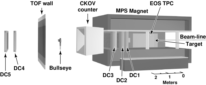
FIG. 1.: E910 layout.

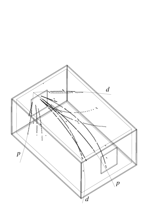
FIG. 2.: 18 GeV/c p+Au event in EOS TPC. Reconstructed tracks are drawn for protons and deuterons which contribute to $N_{grey}$.

FIG. 3.: TPC geometric acceptance as a function of momentum and $\cos(\theta)$.

FIG. 4.: Ionization energy loss vs. momentum of particles with $p<2.4$ GeV/c. The lines delimit the dE/dx particle identification cuts for protons and deuterons described in the text.

FIG. 5.: Acceptance corrected momentum vs. $\cos(\theta)$ distribution for protons.

FIG. 6.: Acceptance corrected momentum distributions for protons and deuterons. Black circles for Au, open squares for Cu, and open triangles for Be target.

FIG. 7.: Acceptance corrected angular distributions for protons and deuterons. Black circles for Au, open squares for Cu, and open triangles for Be target.

FIG. 8.: Momentum and angular distributions for values of $N_{grey}=2,6,8,10$.

FIG. 9.: Event normalized multiplicity distributions $\frac{1}{N}dN/dN_{grey}$ of protons (open circles), deuterons (triangles) and both protons and deuterons (dark circles).

FIG. 10.: a) The probability distributions $P(\nu)$ for the beam proton to encounter $\nu$ collisions with target nucleons calculated for p+Be, p+Cu, and p+Au reactions using two different models: The Glauber results are based on the analytical Glauber model with Wood-Saxon nuclear density distributions and the Hijing results are based on a Monte-Carlo simulation of the collision geometry within the Hijing computer code. b) The $\nu$ distributions from Hijing overlayed with the $N_{grey}$ distributions for all three targets.

FIG. 11.: Log-likelihood fits to the event normalized $N_{grey}$ distributions for Be, Cu, and Au targets with two models: The Geometric Cascade Model (dashed lines) and the Polynomial Model (solid lines).

FIG. 12.: $\overline{\nu}(N_{grey})$ and $\sigma(\nu(N_{grey}))$ generated from the Polynomial Model (solid circles) and the GCM (open circles), and $\overline{\nu}(N_{grey})$ according to the $\overline{\nu}^{2}$ ansatz (solid line) for p+Be, p+Cu and p+Au.

FIG. 13.: $P(N_{grey},\nu)$ contours for two models: The Polynomial Model (top) and the Geometric Cascade Model (bottom). The ten contours for each are separated by factors of $\sqrt{10}$, ranging from 0.0001 to 0.316.

FIG. 14.: Comparison between event normalized slow fragment multiplicity distributions for p+Au reactions obtained from the E910 data and RQMD Monte-Carlo calculations.

FIG. 15.: Chi-Square fits to the event normalized RQMD $N_{grey}$ distributions with two models: The Geometric Cascade Model (dashed) and the Polynomial Model (solid), for both E910 and 4$\pi$ model sets.

FIG. 16.: Comparison between the $\pi(\nu)$ distributions for p+Au reactions obtained with 3 different models: Glauber, Hijing and RQMD.

FIG. 17.: Comparison of $\bar{\nu}(N_{grey})$ and $\sigma(\nu(N_{grey}))$ for RQMD values and GCM and Polynomial fits to the RQMD $N_{grey}$ within the E910 acceptance and over 4$\pi$.

FIG. 18.: Event normalized $N_{grey}$ distributions for a given value of $\nu$ for RQMD tracks in the E910 acceptance, overlayed with the predictions of the two models — dashed for the GCM, and dotted for the Polynomial.

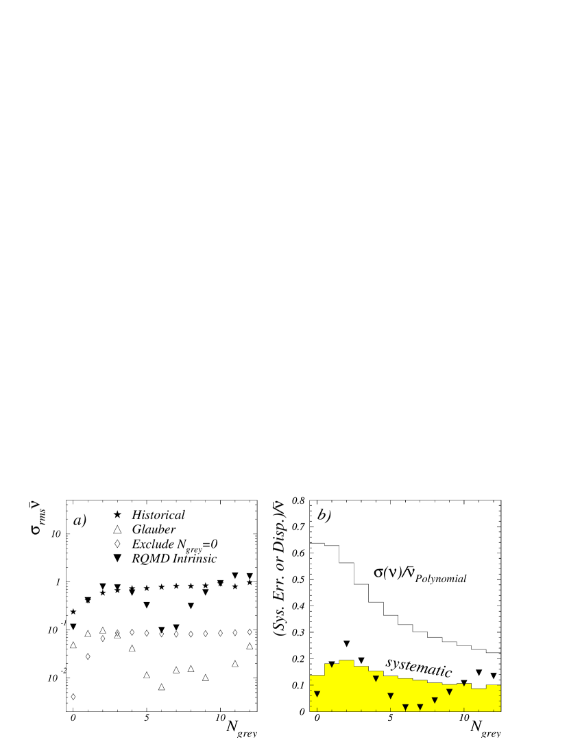
FIG. 19.: a) the rms distribution for $(\overline{\nu}^{\prime}-\overline{\nu})$ as a function of $N_{grey}$, where the prime indicates an alternate set of systematic cuts, or the intrinsic value from RQMD. b) the relative systematic error (shaded) for the combined one standard deviation errors from the three re-analyses described in the text. For comparison the RQMD relative intrinsic difference (triangles) and the polynomial model relative dispersion (unshaded) are also shown.

REFERENCES

- [1] E. Feĭnberg, Jour. Exp. Theor. Phys. 23, 132 (1966).
- [2] A. Dar and Vary, Phys. Rev. D 6, 2412 (1972).
- [3] A. Goldhaber, Phys. Rev. D 7, 765 (1973).
- [4] P. Fishbane and J. Trefil, Phys. Lett. B 51, 139 (1974).
- [5] W. Busza et al., Phys. Rev. Lett 34, 836 (1975).
- [6] J. Elias et al., Phys. Rev. D 22, 13 (1980).
- [7] W. Yeager et al., Phys. Rev. D 16, 1294 (1977).
- [8] W. Busza, in High-Energy Physics and Nuclear Structure, edited by D. Nagle et al. (AIP Conf. Proc., New York, 1975).
- [9] This terminology originates with the identification of emulsion tracks. The grey tracks were those with a grain density between 1.4 and 6.8 times that of minimum ionizing tracks. They peak forward and are composed of protons, deuterons and a few percent tritons, 4He, and mesons. Those with still higher grain density were called balck, and were identified with the proton and nuclear fragments distributed isotropically in the target frame.
- [10] B. Andersson, I. Otterlund, and E. Stenlund, Phys. Lett. B 73, 343 (1978).
- [11] E. Stenlund and I. Otterlund, Nucl. Phys. B198, 407 (1982).
- [12] M. K. Hegab and J. Hufner, Phys. Lett. B 105, 103 (1981).
- [13] M. K. Hegab and J. Hufner, Nucl. Phys. A384, 353 (1982).
- [14] N. Suzuki, Prog. Theor. Phys. 67, 571 (1982).
- [15] J. Babecki and Nowack, Acta Phys. Pol. B 9, 401 (1978).
- [16] C. Rees et al., Z. Phys. C 17, 95 (1983).
- [17] C. DeMarzo et al., Phys. Rev. D 29, 2476 (1984).
- [18] E. Brucker et al., Phys. Rev. D 32, 1605 (1985).
- [19] R. Albrecht et al., Z. Phys. C 57, 37 (1993).
- [20] J. Bailly et al., Z. Phys. C 35, 301 (1987).
- [21] K. Braune et al., Z. Phys. C 13, 191 (1982).
- [22] D. H. Brick et al., Phys. Rev. D 39, 2484 (1989).
- [23] H. Sorge, H. Stoecker, and W. Greiner, Ann. Phys. 192, 266 (1989).
- [24] G. Rai et al., IEEE Trans. Nucl. Sci 37, 56 (1990), lBL-35702.
- [25] J. Hauger et al., Phys. Rev. C 57, 764 (1998).
- [26] K. Nakai et al., Phys. Lett. B 121, 373 (1983).
- [27] N. Porile et al., Phys. Rev. C 39, 1914 (1989).
- [28] A. Hirsch et al., Phys. Rev. C 29, 508 (1984).
- [29] A. Goldhaber, Phys. Lett. B 53, 306 (1974).
- [30] R. Glauber, in High Energy Physics and Nuclear Structure, edited by A. Gideon (North-Holland, Amsterdam, 1967), p. 311.
- [31] X. Wang and M. Gyulassy, Phys. Rev. D 44, 3501 (1991).
- [32] W. Chao, Hegab, and Hufner, Nucl. Phys. A395, 482 (1983).
- [33] M. A. Faessler et al., Nucl. Phys. B157, 1 (1979).