Breakup Conditions of Projectile Spectators from Dynamical Observables

Abstract

Momenta and masses of heavy projectile fragments ($Z\geq 8$), produced in collisions of ¹⁹⁷Au with C, Al, Cu and Pb targets at E/A = 600 MeV, were determined with the ALADIN magnetic spectrometer at SIS. Using these informations, an analysis of kinematic correlations between the two and three heaviest projectile fragments in their rest frame was performed. The sensitivity of these correlations to the conditions at breakup was verified within the schematic SOS-model. For a quantitative investigation, the data were compared to calculations with statistical multifragmentation models and to classical three-body calculations.

With classical trajectory calculations, where the charges and masses of the fragments are taken from a Monte Carlo sampling of the experimental events, the dynamical observables can be reproduced. The deduced breakup parameters, however, differ considerably from those assumed in the statistical multifragmentation models which describe the charge correlations. If, on the other hand, the analysis of kinematic and charge correlations is performed for events with two and three heavy fragments produced by statistical multifragmentation codes, a good agreement with the data is found with the exception that the fluctuation widths of the intrinsic fragment energies are significantly underestimated. A new version of the multifragmentation code MCFRAG was therefore used to investigate the potential role of angular momentum at the breakup stage. If a mean angular momentum of 0.75$\hbar$/nucleon is added to the system, the energy fluctuations can be reproduced, but at the same time the charge partitions are modified and deviate from the data.

I Introduction

In several experiments with the ALADIN spectrometer, the decay of excited projectile spectator matter at beam energies between 400 and 1000 MeV per nucleon was studied [1, 2, 3]. In these collisions, energy depositions are reached which cover the range from particle evaporation to multi-fragment emission and further to the total disassembly of the nuclear matter, the so-called ’rise and fall of multifragment emission’ [4]. The most prominent feature of the multi-fragment decay is the universality that is obeyed by the fragment multiplicities and the fragment charge correlations. These observables are invariant with respect to the entrance channel – i.e. independent of the beam energy and the target – if plotted as a function of $Z_{bound}$, where $Z_{bound}$ is the sum of the atomic numbers $Z_{i}$ of all projectile fragments with $Z_{i}\geq 2$. For different projectiles, the dependence of the fragment multiplicity on $Z_{bound}$ follows a linear scaling law. These observations indicate that compressional effects are only of minor importance. In contrast to central collisions at lower energies, where large radial flow effects are observed, the quantitative interpretation of kinematic observables is therefore simplified.

More important, these characteristics are an indication that chemical equilibrium is attained prior to the fragmentation stages of the reaction. In fact, statistical models were found to be quite successful in describing the experimental fragment yields and charge correlations, if the breakup of an expanded system was assumed [5, 6, 7, 9, 10, 11, 12]. In addition, the temperature of the excited matter, extracted from double ratios of isotope yields, is reproduced. On the other hand, the kinetic energy spectra of particles and fragments are not equally well described within the statistical picture. The energy spectra of light charged particles ($A\leq 4$) can be explained by a thermal emission of the fragments, but their slopes correspond to temperatures approximately three times larger than those extracted from isotope ratios [13]. While this may be an indication for pre-breakup emission if remains to be understood whether the kinetic energies of intermediate mass fragments ($3\leq Z\leq 30$) are consistent with the statistical approach.

The dynamics of the multifragmentation process has therefore to be studied. It is well known that kinematic correlations, which are governed by the long range Coulomb repulsion, are sensitive to the disintegration process. Previous studies concentrated mostly on the two-fragment velocity correlation functions [14, 15, 16, 17, 18, 19, 20, 21, 22]. Only few attempts were made to analyze higher order correlations. However, these studies were done either for heavy fragments at much lower beam energies [23, 24, 25, 26, 27] or for light charged particles only [28]. In this paper, the results of a kinematic analysis of the fragmentation process of the projectile spectator are presented. Heavy projectile fragments produced in peripheral Au induced collisions at E/A = 600 MeV are studied without the influence of energy thresholds of the detectors. Moreover, the analysis is performed in the center of mass frame of the fragments, thus reducing the influence of directed collective motion of the emitting source. On the other hand, a limit of $Z\geq 8$ is imposed for kinematic observables by the lower detection threshold of the TP-MUSIC II tracking detector. The analysis is therefore restricted to the excitation energy range characterized by increasing fragment multiplicities.

II The experiment

A Experimental setup

The experiment was performed with the ALADIN forward spectrometer at the heavy-ion synchrotron SIS of the GSI Darmstadt, using a gold beam with an energy of 600 MeV per nucleon and a typical intensity of 2000 beam particles during a 500 ms spill. A schematic view of the experimental setup in the bending plane of the ALADIN magnet is shown in figure 1. The incoming beam entered the apparatus from the left and first hit the beam counters, where for each beam particle the position in a plane perpendicular to the beam direction and the arrival time were measured with resolutions $\delta_{x}\approx\delta_{y}\approx$ 0.5 mm FWHM and $\delta_{t}$ =100 ps FWHM, respectively. One meter downstream, the reaction target was positioned. Targets of C, Al, Cu and Pb with a thickness between 200 and 700 mg/cm² were used, corresponding to an interaction probability of up to 3%. Light charged particles from the mid-rapidity zone of the reaction were detected by a Si-CsI-array which was placed at angles between 7^o and 40^o with a solid angle coverage of approximately 30% in this angular range ( 50% between 7^o and 25^o, 15% between 25^o and 40^o ). Fragments from the decay of the projectile spectator, emitted into a cone of approximately 5^o around the direction of the incident beam, entered the magnetic field of the magnet. The magnet was operated at a bending power of 1.4 Tm which corresponded to a deflection of 7.2^o for fragments with beam rigidity. The particles were detected in the TOF-wall, which was positioned 6 m behind the target. The time-of-flight of light particles with respect to the beam counter was measured with a resolution of 300 ps FWHM and with a resolution of 140 ps FWHM for particles with a charge of 15 and above. The TOF-wall provided the charge of all detected particles with single element resolution for charges up to eight. Charged particles with charges of eight and above were simultaneously identified and tracked by a time-projecting multiple-sampling ionization chamber TP-MUSIC II ( see section II B ), which was positioned outside the magnetic field between the magnet and the TOF-wall. To minimize the influence of scattering, of energy loss and of secondary nuclear reactions of the fragments after their production in the target, the spectrometer up to an entrance window in front of the ionization chamber was operated in vacuum. The components of the apparatus with the exception of the MUSIC detector have already been described in [1].

B The MUSIC detector

The TP-MUSIC detector is a time-projection multiple-sampling ionization chamber. If a charged particle passes through its active volume, an ionization track containing positive ions – which will drift to the cathode – and free electrons – which will move in the direction of the anodes – is produced. Due to the homogeneous electric field, the drift velocity of the electrons towards the anodes is independent of the position within the gas volume. Therefore, the distance of the primary particle track from the anode is proportional to the time the center of the electron cloud needs to reach the anode. The version TP-MUSIC II [29] which was used in this experiment is shown in figure 2 . It consists of three active volumes with the drift field in adjacent sections perpendicular to each other, two for the measurement of the horizontal and one for that of the vertical position and angle of the particle track. Each field cage has an active area of 100 cm (horizontal) times 60 cm (vertical) and a length of 50 cm. The horizontal field cages are both divided into two halves with a vertical cathode plane in the middle of the detector to reduce the maximum drift length and the high voltages necessary to provide the drift field. The chambers were operated at a high voltage of 150 V/cm, i.e. 7.5 kV for the horizontal and 9 kV for the vertical field cages, P10 ( 90% argon, 10% methane ) at a pressure of 800 mbar served as counting gas. To allow multiple sampling of the particle signals, each anode is subdivided into 16 stripes with a width of 3 cm each.

The anode signals were recorded using flash ADCs with a sampling rate of 16 MHz. Together with a drift velocity of the electrons of approximately 5.3 cm/$\mu$s this corresponds to amplitude measurements at a step size of 3 mm in the direction of the drift. Since the drift time of the electron cloud is measured by each of the 16 anodes of a field cage i.e. at 16 points along the beam direction (z-direction), the complete track information both in x- ( field cage 1 and 3 ) and y-direction ( field cage 2 ) of the primary charged particle inside the MUSIC volume is available. The detector is operated outside the magnetic field volume of the ALADIN magnet, therefore the ionization track through the MUSIC gas is a straight line which is obtained by fitting the 16 track positions by three straight lines - one in each field cage.

The position resolution has been estimated using the fact that the horizontal component of a track is determined with two separate field cages. The intersections of the measured track segments from the first and the third field cage with a virtual reference plane, positioned in the center of the vertical field cage and perpendicular to the z-direction, are calculated. The distance between these two points of intersection is a measure of the overall position and angle resolution of the detector. Its distribution is a gaussian with a width of 2.4 mm FWHM for particles with a charge of 20 and above which increases to approximately 12 mm at the detection threshold of $Z=8$. These values are of the same order of magnitude as the effect of small angle scattering of the fragments in the counting gas of the MUSIC.

The amplitude of the primary signal produced by a particular fragment is proportional to $q^{2}\beta^{2}$, where $\beta$ is the velocity of the particle and $q$ is its charge state. Fragments from the decay of the projectile spectator are moving approximately with beam velocity. In this case, all fragments with nuclear charges up to 50 are fully stripped after passing through the target matter. They remain fully stripped in the detector gas, the primary signal is therefore proportional to the square of the nuclear charge of the particle. For particles with nuclear charges between 50 and 79, the mean charge exchange length in the MUSIC gas ( 8 cm and 30 cm for $Z=50$ and 79, respectively ) is small compared to the path length of the particle within the MUSIC detector. They reach their equilibrium charge state within the detector volume and the primary signal is proportional to the square of the effective charge.

The amplitude of the primary signal decreases due to diffusion broadening ( proportional to the drift distance ) and due to impurities of the counting gas ( proportional to the square of the drift distance ). The amplitude measured at the anode is therefore dependent on the drift distance of the electron cloud. To determine the position correction the incident beam – i.e. particles with known $Z$ and $\beta$ – is swept across the field cages by varying the field of the magnet. In addition, the signals are corrected for the deviations from the beam velocity. This is essential for the charge resolution of binary fission fragments which have the widest distribution of laboratory velocities of all heavy fragments ($Z\geq 8$) from the decay of the projectile spectator. A charge resolution of 0.5 charge units FWHM is reached. This is demonstrated in figure 3 where a charge spectrum of the MUSIC-detector is shown. Since both the differences in pulse height for two neighboring charges and their fluctuations are proportional to $Z$, the charge resolution is independent of the charge of the fragment. The lower threshold for particle identification reached in this experiment is $Z=8$.

C Momentum and mass reconstruction

From the tracks of the charged particles measured behind the ALADIN magnet, the rigidity vector can be determined if the magnetic field is known. It was decided to fit the particle properties as a function of the measured track parameters rather than using a backtracing method because the latter is more time consuming at the analysis stage. For particles with a rigidity vector $\vec{R}$, trajectories starting at the target position $z_{targ}$ and coordinates ($x_{targ}$, $y_{targ}$) within the beam spot are calculated using the routines provided by the program package GEANT [32]. The starting conditions are chosen from a five-dimensional grid with equidistant spacing for the variables $x_{targ}$, $y_{targ}$, $1/R$, $R_{x}/R$ and $R_{y}/R$. For a given magnetic field strength of the ALADIN magnet, the intersection ($x_{music}$, $y_{music}$) of each track with the reference plane of the MUSIC detector and its angle ($m_{x}$, $m_{y}$) relative to this plane as well as the path length to this point are determined. The bending plane of the magnet is the horizontal x-z-plane, i.e. the main component of the magnetic field points to the direction of the y-axis, although the fringe fields can not be neglected, especially if the full geometric acceptance is used.

Since a large range in $N/Z$-ratios (0.7 - 1.5) and emission angles has to be covered, only 40% of the grid points correspond to trajectories which reach the reference plane behind the magnet, all others end at the wall of the magnet chamber where they are lost. For the successful tracks, the three components of the rigidity vector together with the path length are fitted as the product of one-dimensional functions of five variables: the position ($x_{music}$, $y_{music}$), the angle $m_{x}$ and the target position ($x_{targ}$, $y_{targ}$). The fit is done by means of an expansion in series of Chebychev polynomials for each variable. For a magnet which has virtually a dipole field, the most relevant terms are linear in $x_{music}$ and $m_{x}$ for $1/R$, $R_{x}/R$ and the path length, and linear in $y_{music}$ for $R_{y}/R$, but for a accuracy of the momentum reconstruction on the percent level, higher order terms can not be ignored. Under the assumption of an expansion up to third order, approximately 1000 individual contributions have to be calculated, which is not feasible. However, a particular term can be estimated by the size of the related expansion coefficient, since Chebychev polynomials are orthogonal within the interval from -1 to 1, and at the same time all their minima and maxima within this interval have the values -1 and 1, respectively. ( Strictly mathematically speaking, this is not correct. Among other conditions, the orthogonality relations can only be used if the full parameter space is covered. This is not the case, since not all of the tracks reach the reference plane. ) In a second step, small terms are gradually suppressed until the $\chi^{2}$ of the fit has increased by 10%, thus reducing the total number from between 400 to 1000 in the first step ( depending on the highest order taken into account ) to 25 to 40 ( depending on the variable ). The fitting procedure is then repeated using only the remaining relevant terms which leads to slightly different expansion coefficients in the final result.

Once this fitting procedure has been performed for each setting of the magnetic field used during the experiment, the reconstruction of the rigidity vector and of the path length is reduced to the evaluation of a set of polynomials. If a reasonable qualitiy of the reconstruction can be archieved, this is a justification for the somewhat heuristic method to select the relevant contributions. The accuracy can easily be determined by calculating tracks with random start values – i.e. with starting coordinates at the target and for the rigidities not identical with the starting parameters used for the fitting procedure. The reconstruction is done for these tracks by evaluating the fit functions, and the input values are compared to the reconstructed ones. The mean deviations for rigidity and path length are a measure of the uncertainty caused by the reconstruction method itself. Clearly, the size of these deviations is on the one hand dependent on the mesh size of the grid of start values and on the other hand on the choice of the highest order taken into account for the expansion in Chebychev polynomials. Both quantities were optimized until the internal accuracy for all variables was better than 0.1% FWHM within the chosen range of rigidities between 1.2 and 3.6 GeV/c. The final set of coefficients was obtained by fitting $\approx$12000 tracks with a maximum order of 4 for each polynomial and a maximum of 6 for the sum of the orders within a term.

A very similar procedure as described above can be used to estimate the expected errors due to the experimental resolution of the two position detectors in front and behind the magnet. A random offset of the order of the experimental uncertainties is added to the positions and slopes prior to the evaluation of the polynomials. Afterwards, the difference between the reconstructed values with and without random offsets is calculated. The mean value of these deviations is the resolution expected due to the experimental uncertainties. It was found that both an uncertainty of 0.7 mrad and of 3 mm produce an error in the rigidity of 1%. With the time and position resolutions given in the previous section, rigidity resolutions of approximately 1.2% and 3% can be expected for beam particles and medium heavy fragments with charge $\approx$12, respectively. The quality of the rigidity reconstruction can be demonstrated by the rigidity distribution of beam particles passing through the apparatus without any nuclear interaction. Within all targets used in this experiment, gold projectiles reach their equilibrium charge state, providing particles with identical momenta and charge states 77⁺, 78⁺, 79⁺, i.e. with rigidities which differ by 1.3% per charge state. With the carbon target, the influence of angular straggling within the target is small and negligible compared to the experimental errors due to the position resolution. In figure 4, the rigidity distribution of beam particles after passing through the carbon target is plotted versus their x-position in the MUSIC reference plane. In this representation of the data, the three charge states (  equilibrium charge state distribution of 600 MeV/u gold in carbon: 59% of the projectiles are fully stripped, 35% have a charge state of 78⁺ and 6% of 77⁺  [33] ) are clearly visible, i.e. the rigidity resolution for heavy nuclei is approximately 1.3% FWHM which is in agreement with values expected from the resolutions of the individual detectors.

Using the reconstructed values for the rigidity and path length, the charge of the particle measured by the MUSIC detector and the time of flight given by the TOF-wall, the velocity and the momentum vector can be calculated for each charged particle detected both in the MUSIC and the TOF-wall, i.e. for particles with a charge of eight and above. The knowledge of velocity and momentum allows the calculation of the particle’s mass.

In figure 5, the mass spectra for the reactions Au+Al and Au+Cu are shown. Single mass resolution for charges up to 12 is obtained, corresponding to a mass resolution $\Delta$A/A of approximately 4.0% FWHM for light fragments. The dominant contribution to the uncertainty of the mass measurement

$$\frac{\Delta A}{A}=\sqrt{\left(\frac{\Delta R}{R}\right)^{2}+\left(\gamma^{2}\cdot\frac{\Delta TOF}{TOF}\right)^{2}}\quad.$$ (1)

is caused by the mass dependent error of the time measurement which is amplified by the factor $\gamma^{2}$ ( $\gamma^{2}$=2.6 for 600 MeV/nucleon ). From this, a rigidity resolution of 2.4% FWHM can be deduced for light fragments.

III Data

The breakup dynamics of multifragmenting spectator matter will be reflected in the momenta of the fragments produced. Especially observables combining the kinematic information of two or more particles – e.g. relative velocities – are governed by the long-range Coulomb repulsion and are therefore sensitive to time scales of the decay and spatial properties of the decaying source. Clearly, the breakup pattern will change with increasing excitation energy transferred to the spectator matter. From the analysis of reactions of gold projectiles with different targets and beam energies between 400 and 1000 MeV/nucleon it is well established [1, 3, 30] that the quantity $Z_{bound}$ – defined as the sum of the charges of all particles with charge two and above, which are emitted from the projectile spectator and detected in the TOF-wall – reflects directly the size of the spectator as well as the excitation energy transferred to the spectator nucleus. It was furthermore shown that the mean number of fragments produced in a reaction as well as other observables characterizing the populated partition space were independent of the target used, if they were investigated as a function of the quantity $Z_{bound}$. $Z_{bound}$ is therefore used as a sorting parameter describing the violence of the reaction.

As was discussed earlier, momenta and masses could only be reconstructed for particles with a charge $Z$ of eight and above. It will be shown in the next section that events with two and more large fragments with $Z\geq 8$ cover the $Z_{bound}$ range from 30 to 70. The maximum mean number of intermediate mass fragments – defined as fragments with charges between 3 and 30 – is observed for a $Z_{bound}$ value of approximately 40. The dataset available covers therefore the range from peripheral collisions up to the region of maximum fragment production.

A Characterization of two- and three-particle events

To show the characteristics of the event classes with two and three heavy particles with charge $Z\geq 8$, their reaction cross sections $d\sigma/dZ_{bound}$ are plotted in the upper panel of figure 6 for the four different targets as a function of $Z_{bound}$. In the following, events with two (three) fragments with charge $Z\geq 8$ are called binary (ternary). Binary events attributed to binary fission were excluded by the condition that either the lighter fragment is of charge below 20 or the sum of the two charges is smaller than 60. In the $Z_{1}Z_{2}$-plane, this region is well separated from the region of binary fission [34]. For comparison, the inclusive reaction cross sections – i.e. without conditions on fragment multiplicity and charge – are also shown: The binary and ternary events represent approximately 10% and 1% of the nuclear reaction cross section, respectively. In order to demonstrate that binary fission events as defined above populate an impact parameter region different from that of binary events without fission, the cross section for binary fission in the reaction Au+C is included. These events are obviously produced in very peripheral reactions. It had been shown earlier [2] that multifragment events evolve – with decreasing $Z_{bound}$ – from events with one heavy residue in the exit channel of the reaction and not from binary fission events.

The sum of the charges of the two and three fragments is plotted in the lower panels. In ternary events, typically 80% of $Z_{bound}$ is contained in the charges of the three heavy fragments with average charges and masses of $\langle Z_{i}\rangle$ = 22, 13, 10 and $\langle A_{i}\rangle$ = 48, 29, 20, i=1,2,3. In binary events, the sum of the charges of the heavy fragments accounts on average for 75% of Z_bound with a clear minimum at Z_bound=40, where the maximum mean number of intermediate mass fragments is observed. The average charges and masses for this event class are $\langle Z_{i}\rangle$ = 26, 13 and $\langle A_{i}\rangle$ = 57, 27, i=1,2.

It will now be demonstrated that these two event classes are representative subsets of the experimental data, i.e. that for a given $Z_{bound}$ value no evidence for a strong dependence on the number of heavy fragments is found. This means that other quantities defining an event do not show a close correlation between their mean values and the multiplicity of the heavy fragments if analyzed according to $Z_{bound}$. Evidently, only observables can be used for this investigation which are not dominated by autocorrelations. The multiplicity of intermediate mass fragments for instance contains the number of all heavy fragments with a charge smaller than 30. The mean multiplicity of IMFs is therefore influenced by the selection criterion and will be significantly different for events with different numbers of heavy fragments in the exit channel.

The mean number $\langle M_{lp}\rangle$ of light particles from the mid-rapididy zone of the reaction which were detected in the hodoscope is a quantity which is certainly dependent on the violence of the reaction but independent of the specific decay channels of the excited projectile spectator. In figure 7, the inclusive distributions of $\langle M_{lp}\rangle$ versus $Z_{bound}$ for the four targets are shown together with the distributions for events with two and three heavy particles. In agreement with the participant-spectator-model, the size of the interaction zone – represented by the mean number of light particles – increases with decreasing size of the projectile spectator. The distributions are independent of the multiplicity of heavy projectile fragments with the exception of the most peripheral reactions ( $Z_{bound}\geq$ 65 ). In this range of largest impact parameters the inclusive data are dominated by spallation and not by multifragmentation events. There, the restriction to events with two or three heavy particles in the exit channel is synonymous with the selection of events with higher mean energy.

The transversal deflection of the decaying projectile spectator is another quantity which is not influenced by autocorrelations with regard to the decay pattern. Since in events with two or three heavy particles in the exit channel the heavy particles contain typically 75-80% of $Z_{bound}$, the center of mass of these particles is in good approximation the center of mass of the decaying system. Thus, the transversal velocity

$$\beta_{trans}=\sqrt{\beta_{x}^{2}+\beta_{y}^{2}}$$ (2)

of the center of mass of the two or three particles with respect to the beam frame was calculated. In figure 8, the mean values of this velocity as a function of $Z_{bound}$ are compared for events with two and three heavy fragments in the exit channel. In agreement with inclusive measurements at 400 MeV/nucleon [35], $\beta_{trans}$ increases monotonously with decreasing $Z_{bound}$ and establishes the transversal deflection of the projectile spectator and therefore the transversal momentum transfer (bounce) as a measure of the deposition of excitation energy into the spectator matter. Pure Coulomb interaction during a grazing collision would lead to very small values for the bounce between $5\cdot 10^{-4}$c and $4\cdot 10^{-3}$c for C and Pb, respectively. But due to the trigger condition demanding at least one light particle detected in the hodoscope and therefore a nuclear reaction, the bounce does not vanish for $Z_{bound}=80$. The increasing Coulomb repulsion with increasing charge of the target nucleus is nevertheless reflected in the small target dependence. Within the experimental errors, the transversal velocity at a given $Z_{bound}$ is independent of the two decay patterns studied.

The two quantities $\langle M_{lp}\rangle$ and $\beta_{trans}$ describe properties related to the initial reaction phase – the size of the fireball and the excitation energy transferred to the spectator matter. The fact that these quantities are independent of a specific choice of the multiplicity of heavy fragments demonstrates that a restriction to the subset of events, defined by the detection threshold of the MUSIC detector, does not select a non-typical sample of the produced projectile spectators.

B Two- and three-particle observables

From the measured momenta of the heavy fragments the intrinsic momenta $\vec{p}_{cm}(i)$ and velocities $\vec{v}_{cm}(i)$ in the center of mass frame (CM-frame) of the binary or ternary heavy fragment system werde determined. This has primarily the advantage of eliminating the projectile velocity from the analysis. Furthermore, it reduces the influence of directed collective motion on the momenta of the particles. This is especially important if the data are to be compared to calculations with models which do not include linear collective motions. By construction, these momenta are collinear in the case of two and coplanar in the case of three particle events. For the further analysis, a new coordinate system has been chosen such that for each event the momentum vectors lie in the same plane – the xy-plane – and that the direction of the heaviest particle coincides with the x-axis. This eliminates the three Euler angles which describe the spacial orientation of the momenta relative to the beam axis. The kinematics of the two and three heavy fragments is thus reduced to one ( $p_{x}(1)$ ) and three ( $p_{x}(1)$, $p_{y}(2)$, $p_{x}(2)-p_{x}(3)$ ) parameters, respectively. The relative kinematics of the fragments can thus uniquely be expressed in terms of one and three independent quantities which, for the analysis presented in this paper, are chosen as follows: (i) the total kinetic energy $E_{3}$ of the fragments in the CM-frame, (ii) the reduced relative velocity $v_{red}(2,3)$, and (iii) a quantity $\Omega_{\Delta}$ which describes the event shape in velocity space. In the case of only two heavy particles, the kinetic energy $E_{2}$ alone is sufficient to describe the decay dynamics.

The sum $E_{3}$ of the kinetic energies of the three particles is calculated in their CM-frame

$$E_{3}=\sum_{i=1}^{3}\frac{p^{2}_{cm}(i)}{2\cdot m_{0}\cdot A_{i}}\quad,$$ (3)

where $m_{0}$=931.5 MeV/c² is the atomic mass unit and $A_{i}$ the mass number of the fragment $i$. The kinetic energy of the particles is dominated by the Coulomb interaction which itself is strongly dependent on the charges involved. The mean value $\langle E_{3}\rangle$ is therefore studied together with the standard deviation $\sigma_{3}$ of the $E_{3}$-distribution as a function of the nominal Coulomb-repulsion $E_{c}$ of the fragments at the time of the breakup, i.e. as a function of the Coulomb potential of three touching spheres with radii $R_{i}$ = 1.4 $\cdot$ $A_{i}^{1/3}$:

$$E_{c}=e^{2}\cdot\sum_{i<j}\frac{Z_{i}\cdot Z_{j}}{1.4\cdot(A_{i}^{1/3}+A_{j}^{1/3})}\quad.$$ (4)

This is a generalization of the well known Viola formula [31]. For events with only two heavy fragments the kinetic energy and the Coulomb repulsion are calculated accordingly. The experimental results are plotted in figure 9 for the four targets used. Within the statistical uncertainties, no target dependence is apparent. In all further plots, mean values of the kinetic energy and of the width of the energy distribution for the combined data of all four targets will therefore be shown. $\langle E_{2}\rangle$, $\langle E_{3}\rangle$, and $\sigma_{2}$, $\sigma_{3}$ depend linearly on $E_{c}$ and are parameterized in terms of straight line fits ($y=m\cdot x+b$) common to the data of all four targets. The slopes and intercepts of these fits are listed in the following table:

	binary		ternary
mE	0.43	$\pm$ 0.05	0.37	$\pm$ 0.04
bE (MeV)	39.0	$\pm$ 4.0	76.0	$\pm$ 5.0
mσ	0.0	$\pm$ 0.05	-0.07	$\pm$ 0.01
bσ (MeV)	28.0	$\pm$ 3.0	44.0	$\pm$ 4.0

The parameters $b_{E}$ and $b_{\sigma}$ describe the mean energies and their variations in the limit of $E_{c}$=0, i.e. without Coulomb interaction, both for binary and ternary events. Under the assumption of a purely thermal source with a temperature $T$ and without Coulomb interaction the mean values $\langle E_{2}\rangle$ and $\langle E_{3}\rangle$ of the kinetic energy distributions are $2T$ with a width $\sigma_{2}$ of $\sqrt{2}T$ and $4T$ with a width $\sigma_{3}$ of $2T$ in case of surface emission and $3/2\cdot T$ with a width $\sigma_{2}$ of $\sqrt{3/2}T$ and $3T$ with a $\sigma_{3}$ of $\sqrt{3}T$ in case of volume emission of the fragments. For both breakup scenarios, the temperatures deduced from these relations are within the experimental errors identical for binary and ternary events. The assumption of volume emission leads to a temperature of 25 MeV whereas the value for surface emission is 20 MeV. Results obtained in the reaction Au + Au at 1000 MeV/nucleon where kinetic temperatures were extracted from the energy spectra of light charged particles up to ⁴He emitted from the target spectator [13] and temperatures extracted from transverse momentum distributions at 600 MeV/u [3] are of similar size ( 15-20 MeV ).

In line with previous studies [17], the reduced relative velocity is defined as

$$v_{red}(i,j)=\frac{v_{rel}(i,j)}{\sqrt{Z_{i}+Z_{j}}}\quad,$$ (5)

where $v_{rel}(i,j)$ is the relative velocity of particles $i$ and $j$ and $Z_{i}$ and $Z_{j}$ are the corresponding charges of the fragments. With this definition, the mutual Coulomb repulsion within a fragment pair is charge independent. For ternary events, the reduced relative velocity of the second and third largest fragment is calculated. Its mean experimental value, averaged over all targets, is 0.0206$\cdot$c $\pm$ 0.0005$\cdot$c. This value will be used later on to adjust the input parameters of model calculations.

The third quantity $\Omega_{\Delta}$ characterizes the configuration of the three velocity vectors

$$\Omega_{\Delta}=\frac{\Delta_{123}}{\Delta_{0}}\quad,$$ (6)

where $\Delta_{123}$ denotes the area of the triangle with its three sides given by the three relative velocities $\vec{v}_{rel}(1,2)$, $\vec{v}_{rel}(2,3)$, and $\vec{v}_{rel}(1,3)$. The normalization $\Delta_{0}$ represents the area of an equilateral triangle with an circumference of

$$u=|\vec{v}_{rel}(1,2)|+|\vec{v}_{rel}(2,3)|+|\vec{v}_{rel}(1,3)|\quad,$$ (7)

which is the largest area possible for a given circumference. Thus, $\Omega_{\Delta}$ varies between 0 and 1, where $\Omega_{\Delta}$=0 corresponds to a streched configuration with the three relative velocities being collinear and $\Omega_{\Delta}$=1 corresponding to a situation where the three CM-velocities point to the corners of an equilateral triangle. The normalized experimental distributions of the reduced area $\Omega_{\Delta}$ are shown in figure 10 for the four targets: The probability to find an equilateral velocity configuration is two orders of magnitude larger than that for a stretched one. Within the statistical errors, the distributions are independent of the target, therefore the mean value averaged over all four targets was determined to increase the statistics especially for small values of $\Omega_{\Delta}$. In order to address the question of possible correlations between the event shape and the charges of the fragments, the average charges $\langle Z_{i}\rangle$ ($i$=1,2,3) of the three fragments ordered according to their sizes are studied as a function of $\Omega_{\Delta}$ for the combined data of all targets. The results are shown in figure 11. Within the statistics, the average charges are independent of $\Omega_{\Delta}$, indicating that the probability distribution of $\Omega_{\Delta}$ is not a trivial consequence of the charge distribution or the spectator size.

C Sensitivity of the three-particle variables

In order to illustrate the potential sensitivity of the chosen observables, calculations with the schematic SOS-code [36] were performed. This code was especially developped to study the influence of two extreme breakup mechanisms on experimentally observable kinetic quantities, using in both cases a nuclear system of a given size and excitation energy and identical multifragment channels. It produces multifragment events with two sets of momentum distributions, simulating for each event on the one hand a sequence of binary decays and on the other hand a simultaneous breakup using the final partition of the sequential decay chain and placing the fragments randomly but without overlap in a sphere.

For this investigation, masses and excitation energies of the decaying spectator nuclei were chosen according to [5] where the authors adjusted the input parameters of a statistical fragmentation model (Berlin model) until the relation between $\langle M_{imf}\rangle$ and $Z_{bound}$ was well reproduced for the system Au + Cu at 600 MeV/nucleon. Since the main motivation of the calculations using the SOS code was to illustrate the potential usefulness of the presented observables and not to describe the dynamical aspects of the data, no further attempt was done to optimize the input parameters of the code. The standard built-in parameters [36] were used, especially a density for the simultaneous breakup szenario of one half of normal nuclear density which is much larger than the values extracted from statistical multifragmentation models ( $\rho/\rho_{0}$ = 0.3 in the Copenhagen and the Moscow code and 0.135 in the MCFRAG code ).

If the sensitivity of the chosen observables is to be tested, it is – however – important that the simulations provide a sample of Monte Carlo data which matches – with respect to the fragment composition – the experimental data. This is demonstrated in figure 11, where for both breakup scenarios the mean charges $\langle Z_{i}\rangle$ in ternary events, ordered according to their sizes, are compared to the experimental data. The large fluctuations for the simultaneous breakup scenario are due ro the fact that only very few events with small $\Omega_{\Delta}$ values are produced ( see next figure ).

In figure 12, the probability distribution of the quantity $\Omega_{\Delta}$ is shown for both breakup scenarios and the experimental data. As a reference, the $\Omega_{\Delta}$-distribution for a thermal system containing three non-interacting fragments is included. For the simultaneous breakup, the probability of stretched velocity configurations – i.e.  small $\Omega_{\Delta}$ – is significantly smaller than for a purely sequential decay process and for the limit of a thermal system. This difference was to be expected, since the repulsive mutual Coulomb interaction shifts initially stretched velocity configurations to larger values of $\Omega_{\Delta}$. The influence of the Coulomb interaction is especially strong for the relatively small radius used in this simulation, which is already an indication that smaller densities will lead to a better description of the experimental data. Only due to this repulsion, the velocity configuration is an image of the breakup configuration in the coordinate space. Any thermal motion – i.e. any motion which is independent of the relative positions of the fragments – reduces this correlation. For realistic input parameters of the decaying system (see section IV), the correlation coefficient $r(\Omega_{\Delta},X_{\Delta})$ between $\Omega_{\Delta}$ and the equivalent quantity in the coordinate space $X_{\Delta}$

$$r(\Omega_{\Delta},X_{\Delta})=\frac{\langle\Omega_{\Delta}\cdot X_{\Delta}\rangle-\langle\Omega_{\Delta}\rangle\cdot\langle X_{\Delta}\rangle}{\sigma(\Omega_{\Delta})\cdot\sigma(X_{\Delta})}$$ (8)

has values of approximately 0.1. ( Note that even in the case of $T=0$ and three identical charges this coefficient does not reach the value 1.0 since the relation between the distance of two charged particles and their relative momentum due to the Coulomb-repulsion is not linear. ) If – on the other hand – a selfsimilar radial flow dominates the momentum distribution, $r(\Omega_{\Delta},X_{\Delta})$ can reach values around 0.3.

In figure 13, the probability distribution of the reduced relative velocity $v_{red}(2,3)$ between the second and third largest fragments is shown, again both for the data and the SOS calculations. The two scenarios predict significantly different relative velocity distributions which in both cases differ clearly from the data. In particular, the sequential calculations (solid histogram) show a pronounced peak at $v_{red}(2,3)=0.012~{}c$. This structure originates from the direct splitting of an intermediate state into the observed fragments 2 and 3 at a rather late stage of the decay sequence. The absence of this structure in the data may therefore signal either a smearing of the relative velocity between the final fragments 2 and 3 by decays following the splitting into the primordial second and third largest fragments, or proximity effects caused by the presence of other particles, or a different decay mechanism which does not produce fragment 2 and 3 via a binary splitting.

The results presented in figures 12 and 13 suggest that the quantities chosen to describe the dynamics of the multifragment events are sensitive to important characteristics of the decay process. In the following chapter, the experimental results will be compared to calculations with statistical multifagmentation models and classical three-body calculations in order to limit the parameter space of the break-up scenario.

IV Comparison to model calculations

A Statistical multifragmentation models

Since statistical multifragmentation models have been shown to describe the observables in the partition space of the multifragmentation process [2, 5, 6, 7, 8, 13], it is the obvious next step to compare their predictions to the kinetic energy distribution obtained in the present experiment. ( It should be emphasized that the description of the partition space comprises the cross sections for binary and ternary events as defined in III A. ) Results are shown for the Berlin code (MCFRAG) as well as the Copenhagen and the Moscow code. A detailed description of the differences between the three models can be found in reference [37]. An extensive and detailed investigation of all dynamical observables as defined in sections III A and III B was only performed using the statistical multifragmentation code MCFRAG [5].

All three models assume an equilibrated source with a given number of nucleons $A$ at a density $\rho$ with an excitation energy $E^{*}$ per nucleon. This source is non-homogeneous, it consists of regions of liquid with normal nuclear density and regions of gas. To compare the calculations to the experimentally observed decay of the projectile spectator, the global parameters $A$ and $E^{*}$ have to be provided as a function of the impact parameter $b$. To do so, the number of nucleons of the projectile spectator was calculated within a geometrical abrasion picture for the collision Au+Au using a radius parameter of 1.3 fm. The excitation energy for a given spectator size within the three codes was then chosen according to [5, 6, 7]. For the nuclear density at freeze out the standard values of the models were taken, i.e. $\rho/\rho_{0}$ = 0.3 for the Copenhagen and the Moscow code and 0.135 for the MCFRAG code. In figure 14, the size of the projectile spectator and its excitation energy are shown versus the impact parameter. It should be noted that for all three models the excitation energy necessary to describe the partition space of the multifragmentation is significantly smaller than the experimental results obtained for the reaction Au + Au at 600 MeV/nucleon using a total energy balance [30]. The number of events to be produced for each interval in $b$ was chosen according to the geometrical cross section for the interval, $dP(b)\sim bdb$. The impact parameter was varied between 0.5 and 12.0 fm in steps of 0.5 fm. For the MCFRAG code, the calculation of the observables was done twice: First, the output of the simulations was used directly, then random errors on the order of the experimental uncertainties for light particles were added to the masses and momenta of the fragments before the same analysis was performed. In this way, an upper estimation for the uncertainties produced by the experimental resolution was achieved.

In figure 15 the mean kinetic energies $\langle E_{2}\rangle$ and $\langle E_{3}\rangle$ for binary and ternary events ( as defined in III A ) in the center of mass frame of the two or three particles and the widths of these distributions $\sigma_{2}$ and $\sigma_{3}$ are plotted versus the nominal Coulomb energy. In the case of the MCFRAG code, the results including the experimental resolution are shown, for the two other sets of simulations, the uncertainties due to the experimental errors were added quadratically to the intrinsic widths of the energy distributions. The mean kinetic energy $\langle E_{3}\rangle$ is reasonably well described by all models, although small differences arise: For the whole range of $E_{c}$, the calculations using the Copenhagen model is steeper than the experimental distribution, therefore the agreement is, compared to the two other models, worse. The overall agreement of data and the three sets of calculations – independent of internal details in the theoretical treatment of the fragmentation process – and the simultaneous description of $\langle E_{2}\rangle$ and $\langle E_{3}\rangle$ by the MCFRAG code are nevertheless a confirmation for the expansion of the nuclear matter prior to its decay. The width of the energy distributions, on the other hand, is underestimated by almost a factor of two both for events with two and three heavy fragments in the exit channel. In spite of deviations between the three sets of calculations, the inadequate description of $\sigma_{3}$ is a generic problem of all three statistical multifragmentation models. Using the MCFRAG code, it was verified that this underprediction of $\sigma_{3}$ can not be compensated by reasonable fluctuations of the initial excitation energy of a given spectator: Combining the events from three sets of calculations with 0.9, 1.0 and 1.1 times $E^{*}(A_{0})$ does not change the width of the energy distribution. This variation of the excitation energy corresponds within the relevant range of spectator sizes approximately to the width of the energy distribution used in [8] to describe the experimental charge distributions.

In figure 16 the probability distribution for the quantity $\Omega_{\Delta}$ is plotted both for the data and the calculations with the MCFRAG code. The calculated distribution is significantly steeper than the experimental one. On the other hand, it is less steep than the result of the SOS-calculation for a simultaneous breakup presented in figure 12. Since in both cases the excitation energy transferred to the spectator matter of a given size is identical and the breakup pattern is on average very similar, any differences in the velocity distributions are caused by the different radii of the breakup volume. This will result in different contributions from the Coulomb interaction and – more important – in different spacial breakup configurations. On average, an elongated structure will result in a smaller value of $\Omega_{\Delta}$ than a more compact one. If, however, the volume is very small like in the case of the SOS-calculations, elongated configurations are less likely. The probability distribution of $\Omega_{\Delta}$ is therefore expected to be steeper than for the more dilute system used for the MCFRAG-calculations.

B The influence of angular momentum

The simulations presented in the previous section showed that the experimental energy distributions can not be explained in a purely thermal description of the nuclear matter, if the temperature is adjusted to reproduce the charge distributions. It was shown earlier that the coupling of random and collective motion increases the fluctuations of the kinetic energy [38]. As an additional degree of freedom angular momentum was therefore taken into account. It is well known from the study of fission and compound nuclei at lower energies that in heavy ion reactions very large angular momenta can be transferred, causing a collective rotation of the excited matter. INC-calculations at 100 and 200 MeV/nucleon show that the mean angular momentum per nucleon transferred can be as large as 0.75$\hbar$, but even more important than the mean values are the huge angular momentum fluctuations which may reach 0.5$\hbar$ per nucleon FWHM [39]. The influence of angular momentum on the decay pattern of nuclear matter within the framework of statistical fragmentation models has only barely been studied so far.

Calculations with the MCFRAG model were done using a version of the code where the treatment of angular momentum was implemented in a fully microcanonical way [9]. The impact parameter was again varied between 3.0 and 12.0 fm in steps of 0.5 fm ( below 5 fm, no events with three heavy fragments are produced ) and a total number of 570000 events for each set of simulations was produced. In this implementation, the rotational degrees of freedom are assumed to be completely thermalized and the contribution of the intrinsic rotation of the produced fragments to the total angular momentum is neglected. This is supposed to be a good approximation for expanded systems at the time of freeze out, since the main part of the angular momentum is contained in the orbital motion of the fragments around the common center of mass.

Calculations were performed for three nuclear densities 0.055$\rho_{0}$, 0.080$\rho_{0}$, 0.135$\rho_{0}$, using the relations between impact parameter, system size and excitation energy which were already shown in figure 14, and a mean angular momentum $\langle L\rangle$ of 0.75$\hbar$A. The angular momentum transfer was distributed according to

$$P(L)=\frac{L}{0.5\cdot\langle L\rangle}\cdot\exp\left(\frac{-L}{0.5\cdot\langle L\rangle}\right)\quad.$$ (9)

In reference [9], it was already shown that simulations with this angular momentum distribution together with a nuclear density of 0.08$\rho_{0}$ describe simultaneously the quantities $\langle E_{3}\rangle$ and $\sigma_{3}$. The results, again including the influence of the experimental uncertainties, are shown in figure 17 for the three densities listed above. As expected, the mean kinetic energy as well as the width of the energy distribution increases with increasing nuclear density. Due to the fact that the mean rotational energy is not very large, the incorporation of angular momentum does not change $\langle E_{3}\rangle$ very much, as a comparison to figure 15 demonstrates, but the large variation of angular momenta produces nonthermal fluctuations which increase the value of $\sigma_{3}$ significantly, resulting in a good description of both $\langle E_{3}\rangle$ and $\sigma_{3}$ for densities between 0.055$\rho_{0}$ and 0.080$\rho_{0}$. At the same time, the quantity $\Omega_{\Delta}$ is much better described, as is shown in figure 18 where the probability distribution of $\Omega_{\Delta}$ is plotted for the three densities. Independent of the nuclear density chosen the probability for the occurence of stretched configurations of the three velocity vectors is enhanced.

To check whether the decay pattern is changed by the angular momentum, observables which were used in earlier papers [2, 3] to describe the charge partition space of the reaction were investigated: The mean values of the asymmetries

$$a_{12}=\frac{Z_{1}-Z_{2}}{Z_{1}+Z_{2}}\qquad\mbox{and}\qquad a_{23}=\frac{Z_{2}-Z_{3}}{Z_{2}+Z_{3}}\quad,$$ (10)

the mean number of intermediate mass fragments $M_{imf}$ and the average charge of the largest fragment $Z_{max}$ are calculated as a function of $Z_{bound}$. In figure 19, the results are shown for simulations with and without angular momentum together with the experimental data. Whereas the mean number of intermediate mass fragments $\langle M_{imf}\rangle$ does not change very much under the influence of angular momentum, this is not true for the details of the decay pattern of the spectator: The mean asymmetry $\langle a_{12}\rangle$ between the charges of the largest and the second largest fragment decreases dramatically for values of $Z_{bound}$ above 50, which means that the two fragments become more comparable in size. As a consequence, the mean charge of the largest fragment $\langle Z_{max}\rangle$ within an event also decreases. At the same time, the mean asymmetry between the charges of the second and the third largest fragment $\langle a_{23}\rangle$ increases, which means that in the presence of angular momentum the charge of the spectator is more evenly divided between the two largest fragments. The changes in the breakup pattern are more pronounced for a small freeze out density. These results are in qualitative agreement with the investigations presented by Botvina and Gross [9], where the size of the largest fragment and the relative size of the two largest fragments was studied under the influence of different amounts of angular momentum.

From the calculations presented above it is obvious that large angular momenta per nucleon destroy the agreement between the results of the statistical multifragmentation code and the data as far as the partition pattern of the spectator matter is concerned. This is especially true for large values of $Z_{bound}$, i.e. for peripheral collisions. On the other hand, it was shown that the additional degree of freedom increased the fluctuations of the kinetic energy by a substantial amount. The question therefore arises whether a better overall agreement can be achieved if the transfer of angular momentum per nucleon to the system is reduced for large impact parameters.

If the peripheral reactions are treated in the abrasion-ablation picture applying the formalism described in [40], values for the angular momentum transfer are obtained which are smaller than the value of 0.75$\hbar$/nucleon by a factor of 5 to 10. These numbers together with a density of 0.135$\rho_{0}$ result in a reasonable description of the partition but the energy fluctuations are again underestimated. The mean values of the asymmetries $a_{12}$ and $a_{23}$ might suggest that this can be compensated by an increase of the nuclear density at breakup. Unfortunately, this is in contradiction to the description of the quantity $\langle M_{imf}\rangle$. The probability to find large values of $\langle M_{imf}\rangle$ for the $Z_{bound}$ range between 40 and 70 decreases with increasing density. As the mean multiplicity of IMF’s is already too small, a further increase of the density would make the deviations even worse.

This leaves no room for a parametrization of angular momentum transfer and density which fits both aspects of the experimental data. The charge partition space and the dynamics of multifragmentation events can not be described simultaneously by the statistical multifragmentation model even if angular momentum as an additional degree of freedom and therefore as a potential source for fluctuations is taken into account.

The conclusions drawn in this section are valid only for a nuclear system where all degrees of freedom are completely thermalized. If this is not true, i.e. if the time scale for the equilibration of the rotational degrees of freedom is large compared to that of the thermalization of the excitation energy, the process of fragmentation is decoupled from the angular momentum transfer. In this case, the amount of angular momentum transferred to the spectator does not influence the partition space of the reaction, it only contributes to the final momentum distribution of the fragments. Therefore, density and excitation energy on the one hand and angular momentum on the other hand can be adjusted independently and a reasonable agreement with the experimental data can be achieved. This approach has been adopted by the Multics/Miniball group [41]. It has to be stated, though, that with this modification the fragmentation process is not treated in a purely microcanonical picture any longer.

C Classical three-body calculations

A collective radial motion of all constituents of the spectator is another conveivable source of fluctuations of the kinetic energy. If the nuclear matter is compressed in the initial stage of the reaction, an additional nonequilibrated collective contribution to the motion of the nuclear matter will be present [42, 43]. Even though this effect is expected to be small in the peripheral collisions discussed in this paper, values for the radial flow energy up to 1.5 MeV can not be ruled out [3]. First attempts have been made to include collective radial flow in statistical models [44], but a consistent implemention is not yet available. Therefore, classical three-body calculations were performed to get a quantitative estimate for the influence of collective flow.

The simultaneous emission out of a given volume is modeled in the following way: The centers of three non-overlapping fragments with a radius of $1.2\cdot A^{1/3}$ are distributed randomly within a sphere of radius $R$. To each fragment, an isotropically distributed initial velocity is assigned. Constrained by momentum conservation, these velocities were selected according to a probability distribution for the relative kinetic energy

$$P(E)\sim E^{\alpha}\cdot\exp\left(-\frac{E}{T}\right)$$ (11)

with $\alpha$ equals 0.5 or 1.0, corresponding to a volume or a surface emission of the fragments. In addition to this random motion, an initial radial flow velocity

$$\vec{v}_{f,i}=\sqrt{\frac{2\cdot\epsilon_{f}}{m_{0}}}\cdot\frac{\vec{d}_{i}}{R}$$ (12)

was added to the random velocities of the thermal motion. Here, $\vec{d}_{i}$ is the position of the center of fragment $i$ with respect to the center of mass, $\epsilon_{f}$ is the flow energy per nucleon for fragments located at $d_{i}$ = $R$. The charges and masses of the fragments were obtained by a Monte Carlo sampling of the experimental events, thus reducing significantly the uncertainties associated with the fragment distribution. In order to account for the recoil from light particles emitted sequentially from the initial fragments ($Z_{i}^{\prime},A_{i}^{\prime}$), the measured charges $Z_{i}$ and masses $A_{i}$ were multiplied by a factor $(1-T^{2}/(a\cdot\Delta))^{-1}$. For this correction, a level density parameter of $a$=10 MeV was used. The quantity $\Delta$ represents the average energy removed by the emission of a nucleon. For simplicity, $\Delta=2T+E_{s}+E_{b}$ was assumed, where $E_{s}$=8 MeV and $E_{b}$=4 MeV are the typical separation energy and barrier height, respectively. After the interaction of the primordial fragments ($Z_{i}^{\prime},A_{i}^{\prime}$) has ceased, the sequential emission of light particles leading to the observed masses and charges ($Z_{i},A_{i}$) was assumed to take place. For each event, the temperature parameter $T$ was chosen according to the experimental value of $Z_{bound}$ from the relation

$$T=f_{T}\cdot\sqrt{2\cdot(79-Z_{bound})}\quad,$$ (13)

where $f_{T}$ is a free parameter. For $f_{T}$ = 1, the relation describes within the relevant range of $Z_{bound}$ reasonably well the temperatures of the initial projectile spectators as predicted by microscopic transport calculations [46, 45, 2]. A value of 0.75 is in agreement with experimental results obtained by the He-Li isotope thermometer [30, 13]. The paths of the fragments were calculated under the influence of their mutual Coulomb field and two-fragment proximity forces according to Ref. [47]. Since for the further analysis those trajectories were rejected for which the fragments overlapped during the propagation, the influence of the proximity force turned out to be rather small.

In a first step, these schematic trajectory calculations were performed with input parameters corresponding on average to those of the statistical model MCFRAG, i.e. $\alpha=0.5$, $f_{T}\approx$ 0.6 - 0.8, $R\approx$ 7 - 9 fm and $\epsilon_{f}=0$. The results for $\langle E_{3}\rangle$ and $\sigma_{3}$ are comparable to those of the statistical model calculations, especially the width $\sigma_{3}$ is again significantly underpredicted in this case. In order to demonstrate this, the schematic calculations for $f_{T}$ = 0.7, $R$ = 8 fm and $\epsilon_{f}$ = 0 are included in figure 15. The agreement of the classical calculations and the statistical model calculations for a similar set of external parameters is a consistency check and shows in addition that the neglection of the influence of the lighter particles produced in the reaction i.e. the restriction of the experimental investigation to the two or three heaviest fragments does not change the results significantly. The probability distribution of the quantity $\Omega_{\Delta}$ is also compared to the results of the statistical model calculation ( see figure 16 ).

In a next step, the quantities $R$, $\epsilon_{f}$ and $f_{T}$ were varied to fit the experimental data. In order to quantify the agreement between the simulations and the experimental observations, a reduced $\chi^{2}$ was calculated for each parameter set:

$$\chi^{2}=\frac{1}{5}\sum_{i=1}^{5}\frac{(\omega_{i}-\mu_{i})^{2}}{\delta_{i}^{2}}\quad.$$ (14)

Here, $\omega_{i}$ are the four coefficients characterizing the fits to the three-particle data in figure 9 and, in addition, the mean reduced velocity between the two lighter fragments as shown in figure 13. $\delta_{i}$ and $\mu_{i}$ denote the experimental uncertainties of these quantities and the corresponding model predictions, respectively. The result is shown in figure 20. A clear minimum of $\chi^{2}$ can be determined for each given flow parameter $\epsilon_{f}$ by varying independently the other two model parameters $R$ and $f_{T}$. The left part of figure 20 shows in a $R$ - $f_{T}$ plane the contour lines with $\chi^{2}$ = 2 for $\epsilon_{f}$ = 0 ($R\approx$ 15 fm), 0.5 ($R\approx$ 22 fm) and 1 MeV ($R\approx$ 26 fm) and for the two values of the exponent $\alpha$. The corresponding minima of the $\chi^{2}$-distribution are displayed in the right panel of figure 20 as a function of $\epsilon_{f}$. Both for volume emission and surface emission, values for the flow parameter $\epsilon_{f}$ larger than 1 MeV are ruled out whereas the results obtained by values between 0 and 1 MeV show no significant difference in $\chi^{2}_{min}$. To demonstrate the quality of the parameter adjustment, the quantities $\langle E_{3}\rangle$, $\sigma_{3}$ and v${}_{red}(2,3)$ are shown in figure 21 for the parameter set $R$ = 22 fm, $\epsilon_{f}$ = 0.5 MeV and $f_{T}$ = 1.2. In the lower right part of figure 21, $\Omega_{\Delta}$ – which was not used in the fitting procedure – is compared to the experimental values. As expected from the results shown in figures 12 and 16, the probability for the existence of stretched velocity configurations increases with increasing radius of the decaying system. The $\Omega_{\Delta}$-distribution is nevertheless not directly comparable to those shown in figures 12 and 16: They were achieved assuming a fixed breakup density for all decaying systems, whereas the three-body calculations assume a fixed breakup volume.

This set of simulations suggests the disintegration of a highly excited and rather extended nuclear system and very low values of the flow parameter. For $Z_{bound}$=55 – the mean value for events with three heavy particles in the exit channel of the reaction – the fit values correspond to a temperature parameter of approximately 10 MeV and a density below 0.05$\rho_{0}$ which is much smaller than the values used for the MCFRAG calculations in order to reproduce the partition space of the reaction.

In the framework of these schematic calculations the large freeze out radius is due to the balance between Coulomb energy and temperature: If a higher nuclear density is assumed, the Coulomb repulsion is much stronger and requires therefore a compensation by a lower temperature parameter and a vanishing flow to describe the energy spectra. The fluctuations $\sigma_{3}$ of the kinetic energy, on the other hand, reflect in addition to thermal fluctuations also fluctuations due to the position sampling within the breakup volume. Thus, lower temperatures and especially smaller radii lead to a significant reduction of $\sigma_{3}$ which can not be compensated by the small values of radial flow consistent with the energy spectra.

V Conclusions

Kinematic correlations between two and three heavy projectile fragments produced in Au induced reactions at E/A = 600 MeV have been studied. A comparison of the observables to the results of the schematic SOS-model confirms their sensitivity to the disassembly configuration. Classical trajectory calculations sampling the experimental charge distribution limit significantly the possible parameter space of the breakup scenario. Taken at their face values these simulations require highly excited and rather extended nuclear systems at the time of the breakup. These source parameters differ significantly from breakup parameters needed by statistical multifragmentation models in order to describe the observed fragment distributions and mean values of the kinetic energy distributions. On the other hand, these models are not able to reproduce the fluctuations of the energy distribution. Binary events not attributed to binary fission also show fluctuations of the relative kinetic energy which can only be described by the same rather high - and probably unrealistic - thermal contribution. The introduction of angular momentum into the statistical model improves the description of the energy fluctuations, but does not allow anymore to reproduce simultaneously the charge partition.

For any further attempt to reconcile the kinetic observables and the partition pattern of the spectator matter two possible approaches seem conceivable: Either the assumption of a global equilibrium established prior to the fragmentation process is oversimplified and has to be given up, or the statistical models have to be refined.

The nuclear interaction during the breakup process, for example, is so far ignored, the interaction between the fragments is limited to the Coulomb repulsion. ( In the classical three-body trajectory calculations present in this work, a nuclear proximity potential is included, but its influence is strongly suppressed by the requirement that the fragments do not overlap. ) One might speculate that in the case of a stronger overlap of the fragments in an earlier stage of the breakup, the nuclear attractive force between the fragments may partially compensate the Coulomb repulsion. Thus, smaller radii would not necessarily lead to an overestimation of the kinetic energies. First steps to add the nuclear interaction between the fragments to statistical decay models in a consistent manner have already been undertaken [48, 49]. A recent publication suggests that the nuclear interaction is indeed relevant for excitation energies up to approximately 10 MeV/u [50]. At the same time, large fluctuations – similar to dissipative phenomena and shape fluctuations known to be important in binary fission [51] – may arise.

On the long term, a quantitative understanding of fluctuations and their development during the disassembly phase clearly requires dynamical transport models which include a realistic treatment of fluctuations on a microscopic level. Significant progress in the development of microscopic transport models has been achieved during the last decade [52], but only recently first microscopic calculations were published which reproduce for the ALADIN data both the multiplicity of the fragments and the slopes of their kinetic energy spectra [53]. In the framework of this model – and in line with previous studies [54, 55, 56] – it is found that the decaying system is not in thermal equilibrium and that the breakup is dominated by dynamical processes. However, the fragment composition agrees with the experimental one only for a short time interval after the collision (60 fm/c) and is drastically altered during the further time evolution. Thus, a consistent description of the time evolution from the first stages of the collision via the formation of primordial excited fragments to their eventual deexcitation and formation of individual quantum states within one microscopic model is still not available. First attempts to take into account the quantal nature of the nuclear system are being pursued [57, 58, 59] for which the present data may serve as a valuable testing ground.

The authors thank D.H.E. Gross and A.S. Botvina for providing us with their statistical multifragmentation codes and for helpful discussions. This work was partly supported by the Bundesministerium für Forschung und Technologie. J.P. and M.B. acknowledge the financial support of the Deutsche Forschungsgemeinschaft under the Contract no. Po 256/2-1 and Be 1634/1-1.

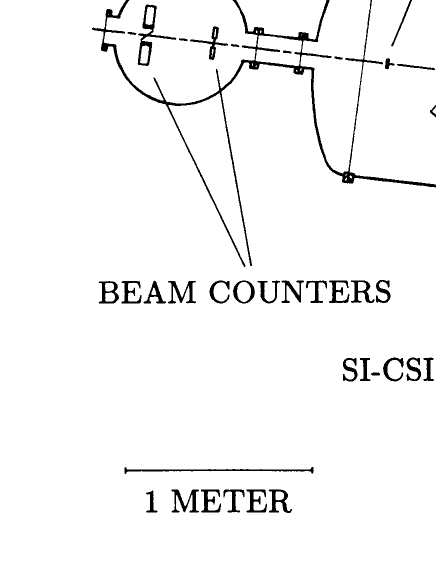
FIG. 1.: Schematic view of the experimental setup in the bending plane of the magnet. The beam enters from the left and hits the beam counters before reaching the target. Mid-rapidity particles are detected in the Si-CsI array. Projectile fragments are tracked and identified in the TP-MUSIC II detector and in the time-of-flight wall.

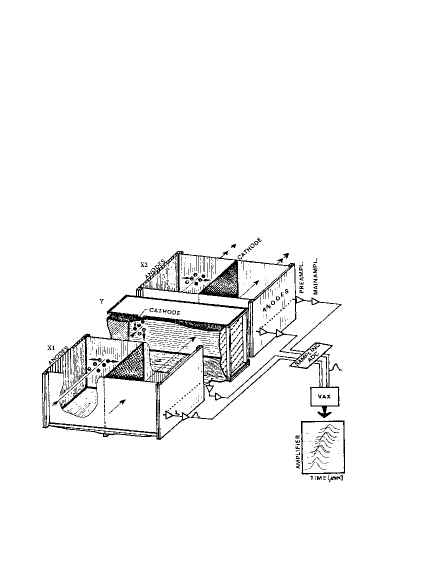
FIG. 2.: Schematic illustration of the design and the operation of the MUSIC II detector. In the first and in the last cage, the electric field is orientated horizontally, in the second field cage vertically, providing the horizontal, the vertical and again the horizontal track information. After amplification and pulse shaping the signals are recorded by a sampling ADC. The insert shows a raw time spectrum as delivered by the 16 anodes of each field cage for a track with a finite angle with respect to the anode plane.

FIG. 3.: Charge spectrum for particles detected by the MUSIC detector in the reaction Au+Cu. Single charge resolution is obtained for the whole range of fragments from the lower detection threshold Z=8 up to beam particles. Fragments with charge 70 and above are suppressed by the trigger conditions.

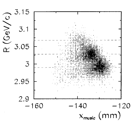
FIG. 4.: Rigidity $R$ of gold projectiles at 600 MeV/nucleon versus the horizontal position in the reference plane of the MUSIC detector. Only events were selected where the gold nuclei passed through the carbon target without any nuclear interaction. The three charge states $79^{+}$, $78^{+}$ and $77^{+}$ correspond to the rigidities 2.990, 3.028 and 3.068 GeV/c, respectively, which are different by 1.3% (dashed lines).

FIG. 5.: Mass spectrum of particles detected in the MUSIC detector for the systems Au+Al and Au+Cu. Single mass resolution is obtained for charges up to 12.

FIG. 6.: (top): Differential cross sections d$\sigma$/d$Z_{bound}$ both for the inclusive data (histograms) and for events with two and three fragments of charge $\geq$8 in the exit channel. For the system Au+C the cross section for binary fission is also shown (solid crosses).
(bottom): Fraction of $Z_{bound}$ contained in the sum of the charges of the two or three heavy fragments versus $Z_{bound}$. The symbols represent a cross section weighted mean value for all four targets.

FIG. 7.: Mean multiplicity $\langle M_{lp}\rangle$ of light particles from the interaction zone of the reaction detected in the hodoscope versus $Z_{bound}$. The histograms show the inclusive distributions for the four targets.
(top): Binary events where binary fission – as defined in the text – was excluded.
(bottom): Ternary events
$\langle M_{lp}\rangle$ decreases with increasing size of the projectile spectator. Within the experimental errors, the multiplicity for a given value of $Z_{bound}$ is independent of the number of the projectile fragments. This holds for the whole range of $Z_{bound}$ with the exception of very peripheral reactions with $Z_{bound}\leq$65 where the inclusive distributions are dominated by spallation reactions.

FIG. 8.: Mean transversal velocity $\beta_{trans}=\sqrt{\beta_{x}^{2}+\beta_{y}^{2}}$ of the center of mass relative to the velocity of the beam for events with two (upper panel) and three (lower panel) heavy particles with $Z_{i}\geq$8 in the exit channel. The bounce decreases with decreasing centrality of the reaction. The non-zero value for the largest $Z_{bound}$ bins is due to the trigger condition which requests the detection of at least one light particle in the hodosope. The dashed lines in both panels show the same linear fit to the binary data, to demonstrate that for a given value of $Z_{bound}$ the distributions do not depend on the multiplicity of heavy particles.

FIG. 9.: (left panels): Mean value $\langle E_{3}\rangle$ (top) and the standard deviation $\sigma_{3}$ (bottom) of the total kinetic energy as a function of the nominal Coulomb energy $E_{c}$ for events with three large fragments in the exit channel of the reaction.
(right panels): $\langle E_{2}\rangle$ (top) and the standard deviation $\sigma_{2}$ (bottom), the equivalent quantities for events with two large fragments where binary fission is excluded.
The results are shown for the systems Au+C, Al, Cu and Pb at E/A = 600 MeV. Both the mean kinetic energy and the width of the energy distribution are within the experimental errors independent of the target. The straight lines are least square fits to the combined data of all targets.

FIG. 10.: Experimental probability distributions for $\Omega_{\Delta}$. The symbols for the combined data of all targets are shifted by 0.02 in x-direction. The event shape in velocity space for large and small values of $\Omega_{\Delta}$ are indicated schematically in the upper left and right corners.

FIG. 11.: Mean values of $Z_{i}$ (i=1,2,3) as a function of $\Omega_{\Delta}$ for the combined data of all targets (symbols). Also included are the results of calculations with the SOS-model assuming a sequential (solid histograms) and a simultaneous (dashed histograms) decay of the projectile spectator ( see section III C ). For all three fragments, the mean charges are independent of $\Omega_{\Delta}$, showing that the probability distribution for $\Omega_{\Delta}$ is not a trivial consequence of the charge distributions.

FIG. 12.: Probability distribution of the observable $\Omega_{\Delta}$. The stars refer to the combined data of all targets. Predictions of the SOS-code assuming a sequential or prompt break-up are shown by the solid and dashed histograms, respectively. Also included are the values for a thermal system without Coulomb interaction. (filled circles).

FIG. 13.: Probability distribution of the reduced relative velocity $v_{red}(2,3)$ between the second and third largest fragment. The symbols refer to the combined data of all targets. Predictions of the SOS-code assuming a sequential or prompt break-up are shown by the solid and dashed histograms, respectively.

FIG. 14.: Input parameters for the simulations with statistical multifragmentation codes.
(top): Size of the decaying spectator $A_{0}$ versus the impact parameter $b$.
(bottom): Excitation energy $E^{*}$ per nucleon versus the impact parameter. The short dashed, long dashed and solid lines show the values used for the three codes COPENHAGEN, MOSCOW and BERLIN, respectively.

FIG. 15.: Mean kinetic energies $\langle E_{3}\rangle$ and $\langle E_{2}\rangle$ (top) and the standard deviations $\sigma_{3}$ and $\sigma_{2}$ (bottom) as a function of the nominal Coulomb-energy $E_{c}$. The symbols denote the experimental data averaged over the reactions Au+C, Al, Cu and Pb. The short dashed, long dashed and solid histograms present predictions of the COPENHAGEN, MOSCOW and MCFRAG fragmentation models, respectively. The dashed-dotted line shows the result of a classical trajectory calculation as described in section IV C. All calculations underpredict significantly the width of the energy distribution while the mean value of the kinetic energy is well described.

FIG. 16.: Probability distribution for $\Omega_{\Delta}$. The symbols denote the experimental data, the histograms model calculations: The solid line represents the calculation with the MCFRAG code using the standard input parameters of the model. The dashed-dotted line shows the result of a classical trajectory calculation as described in section IV C, where the same input parameters were used.

FIG. 17.: Mean kinetic energy $\langle E_{3}\rangle$ and the standard deviation $\sigma_{3}$ as a function of the nominal Coulomb energy $E_{c}$ under the assumption of a mean angular momentum transfer to the spectator of 0.75$\hbar$/nucleon. The dotted, dashed and solid histograms present MCFRAG-calculations with freeze out densities of 0.055$\rho_{0}$, 0.080$\rho_{0}$ and 0.135$\rho_{0}$, respectively. The symbols represent the experimental data.

FIG. 18.: Probability distribution for $\Omega_{\Delta}$ under the assumption of a mean angular momentum transfer to the spectator of 0.75$\hbar$/nucleon. The dotted, dashed and solid histograms present MCFRAG-calculations with freeze out densities of 0.055$\rho_{0}$, 0.080$\rho_{0}$ and 0.135$\rho_{0}$, respectively. The symbols denote the experimental data.

FIG. 19.: Mean charge asymmetry between the two largest fragments $\langle a_{12}\rangle$ (top left) and between the second and third largest fragment $\langle a_{23}\rangle$ (top right), mean number of intermediate mass fragments $\langle M_{imf}\rangle$ (bottom left) and mean charge of the largest fragment $\langle Z_{max}\rangle$ (bottom right) versus $Z_{bound}$ under the assumption of a mean angular momentum transfer to the spectator of 0.75$\hbar$/nucleon. The stars denote the experimental data. The dotted, dashed and solid histograms present calculations with freeze out densities of 0.055$\rho_{0}$, 0.080$\rho_{0}$ and 0.135$\rho_{0}$, respectively. For comparison, the results of calculations without angluar momentum transfer and a freeze out density of 0.135$\rho_{0}$ are included as open circles.

FIG. 20.: Parameter adjustment for the classical three-body calculations. The solid lines correspond to surface emission ($\alpha=1.0$), whereas the dashed lines show the results for volume emission ($\alpha=0.5$).
(left): Contour lines for $\chi^{2}$=2 in a plane defined by the volume radius R and the scaling factor $f_{T}$ of the temperature for flow parameters $\epsilon_{f}$= 0.0, 0.5 and 1.0 MeV.
(right): Minima of the $\chi^{2}$-distribution as a function of $\epsilon_{f}$. Values of $\epsilon_{f}$ larger than 1 MeV are ruled out whereas values between 0 and 1 MeV show no significant differences in $\chi^{2}_{min}$.

FIG. 21.: Mean kinetic energy $\langle E_{3}\rangle$ and its standard deviation $\sigma_{3}$, $v_{red}(2,3)$ and $\Omega_{\Delta}$ for classical three-body calculations (histograms). The parameter set $R$=22 fm, $\epsilon_{f}$= 0.5 and $f_{T}$=1.2, corresponding to the minimum in $\chi^{2}$ in the case of surface emission of the three fragments ( $\alpha=1.0$ ) was chosen. The symbols represent the experimental data.

REFERENCES

- [1] J. Hubele, P. Kreutz, J.C. Adloff, M. Begemann-Blaich, P. Bouissou, G. Imme, I. Iori, G.J. Kunde, S. Leray, V. Lindenstruth, Z. Liu, U. Lynen, R.J. Meijer, U. Milkau, A. Moroni, W.F.J. Müller, C. Ngô, C.A. Ogilvie, J. Pochodzalla, G. Raciti, G. Rudolf, H. Sann, A. Schüttauf, W. Seidel, L. Stuttge, W. Trautmann, A. Tucholski, Z. Phys. A 340, 263 (1991).
- [2] P. Kreutz, J.C. Adloff, M. Begemann-Blaich, P. Bouissou, J. Hubele, G. Imme, I. Iori, G.J. Kunde, S. Leray, V. Lindenstruth, Z. Liu, U. Lynen, R.J. Meijer, U. Milkau, A. Moroni, W.F.J. Müller, C. Ngô, C.A. Ogilvie, J. Pochodzalla, G. Raciti, G. Rudolf, H. Sann, A. Schüttauf, W. Seidel, L. Stuttge, W. Trautmann, A. Tucholski, Nucl. Phys. A556, 672 (1993).
- [3] A. Schüttauf, W.D. Kunze, A. Wörner, M. Begemann-Blaich, Th. Blaich, D.R. Bowman, R.J. Charity, A. Cosmo, A. Ferrero, C.K. Gelbke, C. Groß, W.C. Hsi, J. Hubele, G. Immé, I. Iori, J. Kempter, P. Kreutz, G.J. Kunde, V. Lindenstruth, M.A. Lisa, W.G. Lynch, U. Lynen, M. Mang, T. Möhlenkamp, A. Moroni, W.F.J. Müller, M. Neumann, B. Ocker, C.A. Ogilvie, G.F. Peaslee, J. Pochodzalla, G. Raciti, F. Rosenberger, Th. Rubehn, H. Sann, C. Schwarz, W. Seidel, V. Serfling, L.G. Sobotka, J. Stroth, L. Stuttgé, S. Tomasevic, W. Trautmann, A. Trzcinski, M.B. Tsang, A. Tucholski, G. Verde, C.W. Williams, E. Zude, B. Zwieglinski, Nucl. Phys. A607, 457 (1996).
- [4] C.A. Ogilvie, J.C. Adloff, M. Begemann-Blaich, P. Bouissou, J. Hubele, G. Imme, I. Iori, P. Kreutz, G.J. Kunde, S. Leray, V. Lindenstruth, Z. Liu, U. Lynen, R.J. Meijer, U. Milkau, W.F.J. Müller, C. Ngô, J. Pochodzalla, G. Raciti, G. Rudolf, H. Sann, A. Schüttauf, W. Seidel, L. Stuttge, W. Trautmann, A. Tucholski, Phys. Rev. Lett. 67, 1214 (1991).
- [5] Bao-An Li, A.R. DeAngelis, D.H.E. Gross, Phys. Lett. B 303, 225 (1993).
- [6] H.W. Barz, W. Bauer, J.P. Bondorf, A.S. Botvina, R. Donangelo, H. Schulz, K. Sneppen, Nucl. Phys. A561, 466 (1993).
- [7] A.S. Botvina and I.N. Mishustin, Phys. Lett. B 294, 23 (1992).
- [8] A.S. Botvina, I.N. Mishustin, M. Begemann-Blaich, J. Hubele, G. Imme, I. Iori, P. Kreutz, G.J. Kunde, W.D. Kunze, V. Linddenstruth, U. Lynen, A. Moroni, W.F.J. Müller, C.A. Ogilvie, J. Pochodzalla, G. Raciti, Th. Rubehn, h. Sann, A. Schüttauf, W. Seidel, W. Trautmann, A. Wörner, Nucl. Phys. A584, 737 (1995).
- [9] A.S. Botvina and D.H.E. Gross, Nucl. Phys. A592, 257 (1995).
- [10] A.S. Botvina, A.S. Il’inov, I.N. Mishustin, Yad. Fiz. 42, 1127 (1985) (Sov. J. Nucl. Phys. 42, 712 (1985)).
- [11] J. Bondorf, R. Donangelo, I.N. Mishustin, C.J. Pethick, H. Schulz, K. Sneppen, Nucl. Phys. A443, 321 (1985).
- [12] D.H.E. Gross, Zhang Xiao-ze, Xu Shu-yan, Phys. Rev. Lett. 56, 1544 (1986).
- [13] Hongfei Xi, T. Odeh, R. Bassini, M. Begemann-Blaich, A.S. Botvina, S. Fritz, S.J. Gaff, C. Groß, G. Immé, I. Iori, U. Kleinevoß, G.J. Kunde, W.D. Kunze, U. Lynen, V. Maddalena, M. Mahi, T. Möhlenkamp, A. Moroni, W.F.J. Müller, C. Nociforo, B. Ocker, F. Petruzzelli, J. Pochodzalla, G. Raciti, G. Riccobene, F.P. Romano, Th. Rubehn, A. Saija, M. Schnittker, A. Schüttauf, C. Schwarz, W. Seidel, V. Serfling, C. Sfienti, W. Trautmann, A. Trzcinski, G. Verde, A. Wörner, B. Zwieglinski, accepted for publication in Z. Phys. A.
- [14] R. Trockel, U. Lynen, J. Pochodzalla, W. Trautmann, N. Brummund, E. Eckert, R. Glasow, K.D. Hildenbrand, K.H. Kampert, W.F.J. Müller, D. Pelte, H.J. Rabe, H. Sann, R. Santo, H. Stelzer, R. Wada, Phys. Rev. Lett. 59, 2844 (1987).
- [15] D.H.E. Gross, G. Klotz-Engmann, H. Oeschler, Phys. Lett. B 224, 29 (1989).
- [16] Y.D. Kim, R.T. de Souza, D.R. Bowmann, N. Carlin, C.K. Gelbke, W.G. Gong, W.G. Lynch, L. Phair, M.B. Tsang, F. Zhu, S. Pratt, Phys. Rev. Lett. 67, 14 (1991).
- [17] Y.D. Kim, R.T. de Souza, D.R. Bowmann, N. Carlin, C.K. Gelbke, W.G. Gong, W.G. Lynch, L. Phair, M.B. Tsang, F. Zhu, Phys. Rev. C 45, 338 (1992).
- [18] D.R. Bowman, G.F. Peaslee, N. Carlin, R.T. de Souza, C.K. Gelbke, W.G. Gong, Y.D. Kim, M.A. Lisa, W.G. Lynch, L. Phair, M.B. Tsang, C. Williams, N. Colonna, K. Hanold, M.A. McMahan, G.J. Wozniak, L.G. Moretto, Phys. Rev. Lett. 70, 3534 (1993).
- [19] E. Bauge, A. Elmaani, R.A. Lacey, J. Lauret, N.N. Ajitanand, D. Craig, M. Cronqvist, E. Gualtieri, S. Hannuschke, T. Li, B. Llope, T. Reposeur, A. Vander Molen, G.D. Westfall, J.S. Winfield, J. Yee, S. Yennello, A. Nadasen, R.S. Tickle, E. Norbeck, Phys. Rev. Lett. 70, 3705 (1993).
- [20] B. Kämpfer, R. Kotte, J. Mösner, W. Neubert, D. Wohlfarth, J.P. Alard, Z. Basrak, N. Bastid, I.M. Belayev, Th. Blaich, A. Buta, R. Caplar, C. Cerruti, N. Cindro, J.P. Coffin, P. Dupieux, J. Erö, Z.G. Fan, P. Fintz, Z. Fodor, R. Freifelder, L. Fraysse, S. Frolov, A. Gobbi, Y. Grigorian, G. Guillaume, N. Herrmann, K.D. Hildenbrand, S. Hölbling, A. Houari, S.C. Jeong, M. Jorio, F. Jundt, J. Kecskemeti, P. Koncz, Y. Korchagin, M. Krämer, C. Kuhn, I. Legrand, A. Lebedev, C. Maguire, V. Manko, T. Matulewicz, G. Mgebrishvili, D. Moisa, G. Montaru, I. Montbel, P. Morel, D. Pelte, M. Petrovici, F. Rami, W. Reisdorf, A. Sadchikov, D. Schüll, Z. Seres, B. Sikora, V. Simion, S. Smolyankin, U. Sodan, K. Teh, R. Tezkratt, M. Trzaska, M.A. Vasileiv, P. Wagner, J.P. Wessels, T. Wienold, Z. Wilhelmi, A.L. Zhilin, Phys. Rev. C 48, R955 (1993).
- [21] Bao-An Li, D.H.E. Gross, V. Lips, H. Oeschler, Phys. Lett. B 335, 1 (1994).
- [22] O. Schapiro, D.H.E. Gross, Nucl. Phys. A573, 143 (1994).
- [23] P. Glässel, D. v. Harrach, H.J. Specht, L. Grodzins, Z. Phys. A 310, 189 (1983).
- [24] D. Pelte, U. Winkler, M. Bühler, B. Weissmann, A. Gobbi, K.D. Hildenbrand, H. Stelzer, R. Novotny, Phys. Rev. C 34, 1673 (1986).
- [25] R. Bougault, J. Colin, F. Delaunay, A. Genoux-Lubain, A. Hajfani, C. Le Brun, J.F. Lecolley, M. Louvel J.C. Steckmeyer, Phys. Lett. B 232, 291 (1989).
- [26] G. Bizard, D. Durand, A. Genoux-Lubain, M. Louvel, R. Bougault, R. Brou, H. Doubre, Y. El-Masri, H. Fugiwara, K. Hagel, A. Hajfani, F. Hanappe, S. Jeong, G.M. Jin, S. Kato, J.L. Laville, C. Le Brun, J.F. Lecolley, S. Lee, T. Matsuse, T. Motobayashi, J.P. Patry, A. Péghaire, J. Péter, N. Prot, R. Regimbart, F. Saint-Laurent, J.C. Steckmeyer, B. Tamain, Phys. Lett. B 276, 413 (1992).
- [27] M. Bruno, M.D’Agostino, M.L. Fiandri, E. Fuschini, L. Manduci, P.F. Mastinu, P.M. Milazzo, F.Gramegna, A.M.J. Ferrero, F. Gulminelli, I. Iori, A. Moroni, R. Scardaoni, P. Buttazzo, G.V. Margagliotti, G. Vannini, G. Auger, E. Plagnol, Nucl. Phys. A576, 138 (1994).
- [28] J. Lauret and R.A. Lacey, Phys. Lett. B 327, 195 (1994).
- [29] G. Bauer, F. Bieser, F.P. Brady, J.C. Chance, W.F. Christie, M. Gilkes, V. Lindenstruth, U. Lynen, W.F.J. Müller, J.L. Romero, H. Sann, C.E. Tull, P. Warren, Nucl. Instr. and Meth. A 386, 249 (1997).
- [30] J. Pochodzalla, T. Möhlenkamp, T. Rubehn, A. Schüttauf, A. Wörner, E. Zude, M. Begemann-Blaich, Th. Blaich, H. Emling, A. Ferrero, C. Groß, G. Imme, I. Iori, G.J. Kunde, W.D. Kunze, V. Lindenstruth, U. Lynen, A. Moroni, W.F.J. Müller, B. Ocker, G. Raciti, H. Sann, C. Schwarz, W. Seidel, V. Serfling, J. Stroth, W. Trautmann, A. Trzcinski, A. Tucholski, G. Verde, B. Zwieglinski, Phys. Rev. Lett. 75, 1040 (1995).
- [31] V.E. Viola, T. Sikkeland, Phys. Rev. 130, 2044 (1963).
- [32] R. Brun, F. Bruyant, M. Maire, A.C. McPherson, P. Zanarini, GEANT3 Report, CERN/DD/ec/84-1, (1986).
- [33] Th. Stöhlker, H. Geissel, H. Folger, C. Kozhuharov, P.H. Mokler, G. Münzenberg, D. Schardt, Th. Schwab, M. Steiner, H. Stelzer, K. Sümmerer, Nucl. Instr. and Meth. B 61, 408 (1991).
- [34] T. Rubehn, R. Bassini, M. Begemann-Blaich, Th. Blaich, A. Ferrero, C. Groß, G. Imme, I. Iori, G.J. Kunde, W.D. Kunze, V. Lindenstruth, U. Lynen, T. Möhlenkamp, L.G. Moretto, W.F.J. Müller, B. Ocker, J. Pochodzalla, G. Raciti, S. Reito, H. Sann, A. Schüttauf, W. Seidel, V. Serfling, W. Trautmann, A. Trzcinski, G. Verde, A. Wörner, E. Zude, B. Zwieglinski, Phys. Rev. C 53, 3143 (1996).
- [35] G.J. Kunde, PhD thesis (University Frankfurt) 1994.
- [36] J.A. López and J. Randrup, Comp. Phys. Communications 70, 92 (1992).
- [37] D.H.E. Gross and K. Sneppen, Nucl. Phys. A567, 317 (1994).
- [38] U. Milkau, M. Begemann-Blaich, E.-M. Eckert, G. Imme, P. Kreutz, A. Kühmichel, M. Lattuada, U. Lynen, C. Mazur, W.F.J. Müller, J.B. Natowitz, C. Ngô, J. Pochodzalla, G. Raciti, M. Ribrag, H. Sann, W. Trautmann, R. Trockel, Z. Phys. A 346, 227 (1993).
- [39] Th. Blaich, M. Begemann-Blaich, M.M. Fowler, J.B. Wilhelmy, H.C. Britt, D.J. Fields, L.F. Hansen, M.N. Namboodiri, T.C. Sangster, Z. Fraenkel, Phys. Rev. C 45, 689 (1992).
- [40] J.-J. Gaimard, K.-H. Schmidt, Nucl. Phys. A531, 709 (1991).
- [41] M. D’Agostino, M. Bruno, N. Colonna, A. Ferrero, M.L. Fiandri, E. Fuschini, F. Gramegna, I. Iori, L. Manduci, G.V. Margagliotti, P.F. Mastinu, P.M. Milazzo, A. Moroni, F. Petruzelli, R. Rui, G. Vannini, J.D. Dinius, C.K. Gelbke, T. Glasmacher, D.O. Handzy, W. Hsi, M. Huang, G.J. Kunde, M.A. Lisa, W.G. Lynch, C.P. Montoya, G.F. Peaslee, L. Phair, C. Schwarz, M.B. Tsang, C. Williams, A.S. Botvina, P. Desesquelles, I. Mishustin, Proceedings of the XXXV. International Winter Meeting on Nuclear Physics, Bormio, ed. I. Iori (Ricerca Scientifica ed Educatione Permanente, Milano), 276 (1997).
- [42] J. Hofmann, W. Scheid, W. Greiner, Il Nuovo Cimento 33, 343 (1976).
- [43] G. Poggi for the FOPI-Collaboration, Nucl. Phys. A586, 755 (1995).
- [44] Subrata Pal, S.K. Samaddar, J.N. De, Nucl. Phys. A 49, 608 (1996).
- [45] J. Hubele, P. Kreutz, V. Lindenstruth, J.C. Adloff, M. Begemann-Blaich, P. Bouissou, G. Imme, I. Iori, G.J. Kunde, S. Leray, Z. Liu, U. Lynen, R.J. Meijer, U. Milkau, A. Moroni, W.F.J. Müller, C. Ngô, C.A. Ogilvie, J. Pochodzalla, G. Raciti, G. Rudolf, H. Sann, A. Schüttauf, W. Seidel, L. Stuttge, W. Trautmann, A. Tucholski, R. Heck, A.R. DeAngelis, D.H.E. Gross, H.R. Jaqaman, H.W. Barz, H. Schulz, W.A. Friedman, R.J. Charity, Phys. Rev. C 46, R1577 (1992).
- [46] W. Bauer, Phys. Rev. C 38, 1297 (1988).
- [47] J.A. López and J. Randrup, Nucl. Phys. A503, 183 (1989).
- [48] L. Satpathy, M. Mishra, A. Das, M. Satpathy, Phys. Lett. B 237, 181 (1990).
- [49] A. Das, M. Mishra, M. Satpathy, L. Satpathy, J. Phys. G 19, 319 (1993).
- [50] C.B. Das, A. Das, M. Satpathy, L. Satpathy, Phys. Rev. C 56, 1444 (1997).
- [51] For a recent review see F. Gönnenwein, The Nuclear Fission Process, Edt. C. Wagemans, CRC Press, Boca Raton, 287 (1991).
- [52] See e.g. The Nuclear Equation of State, Part A and B, Edt. W. Greiner and H. Stöcker, Plenum Press, New York (1989).
- [53] P.B. Gossiaux, R. Puri, Ch. Hartnack, J. Aichelin, Nucl. Phys. A619, 379 (1997).
- [54] D.H. Boal, J.N. Gosli, C. Wicentowich, Phys. Rev. Lett. 62, 737 (1989).
- [55] D.H. Boal, J.N. Gosli, C. Wicentowich, Phys. Rev. C 40, 601 (1989).
- [56] G.J. Kunde, J. Pochodzalla, J. Aichelin, E. Berdermann, B. Bethier, C. Cerruti, C.K. Gelbke, J. Hubele, P. Kreutz, S. Leray, R. Lucas, U. Lynen, U. Milkau, W.F.J. Müller, C. Ngô, C.H. Pinkenburg, G. Raciti, H. Sann, W. Trautmann, Phys. Lett. B 272, 202 (1991).
- [57] A. Ohnishi and J. Randrup, Phys. Lett. B 394, 260 (1997).
- [58] J. Schnack and H. Feldmeier, Prog. Part. Nucl. Phys. 39, 393 (1997).
- [59] J. Schnack and H. Feldmeier, Phys. Lett. B 409, 6 (1997).