The Liquid Scintillator Neutrino Detector and LAMPF Neutrino Source

Abstract

A search for neutrino oscillations of the type $\bar{\nu}_{\mu}\to\bar{\nu}_{e}$ has been conducted at the Los Alamos Meson Physics Facility using $\bar{\nu}_{\mu}$ from muon decay at rest. Evidence for this transition has been reported previously. This paper discusses in detail the experimental setup, detector operation and neutrino source, including aspects relevant to oscillation searches in the muon decay-at-rest and pion decay in flight channels.

29.40.Me,14.60.Pq,13.15.tg

1.  Introduction

1.1  Motivation

Standard electroweak theory has three lepton families, each with a charged and neutral partner. It is widely accepted that lepton family number is conserved and so these families are not expected to transform into one another. The minimal theory also assumes that neutrino masses are zero, providing a natural explanation for the left-handed character of the weak interaction. In the last few years it has gradually become accepted that the standard model may well need to be extended to accept finite neutrino mass. The deficit of solar neutrinos and indications from anomalies in atmospheric neutrino events have raised expectations that neutrino oscillations may occur, implying lepton family number mixing and finite neutrino masses. A search for neutrino oscillations has been conducted with the apparatus described in this paper, both from neutrinos generated by muon decay at rest as well as those from pion decay in flight. The source is unique in that the backgrounds expected from conventional processes are very small.

1.2  Experimental Method

The Liquid Scintillator Neutrino Detector (LSND) was designed to detect neutrinos originating in a proton target and beam stop at the Los Alamos Meson Physics Facility (LAMPF). The primary goal was to search for transitions from muon-type to electron-type neutrinos in two complementary ways. The LSND experiment was proposed [1] for this purpose in 1989 and first operated in 1993. First results have been published [2] on the search for the appearance of $\bar{\nu}_{e}$ from the large flux of $\bar{\nu}_{\mu}$ from muon decay at rest (DAR). A search is also being conducted for electron neutrinos in a dominantly ${\nu_{\mu}}$ beam from pions that decay in flight (DIF) [3]. This paper focuses on the apparatus that was used in both searches. Details of the experiment are included that could not appear in a more compressed format.

For the“at rest” experimental strategy to be successful, the target had to be a copious source of $\bar{\nu}_{\mu}$ in a particular energy range of interest with relatively few $\bar{\nu}_{e}$ produced by conventional means. The detector had to be able to recognize interactions of $\bar{\nu}_{e}$ with precision and separate them from other neutrino types, including the large rate of ${\nu_{e}}$ expected from the target. The observation of $\bar{\nu}_{e}$ in excess of the number expected from conventional sources may be interpreted as evidence for neutrino oscillations. However, although we will concentrate on the oscillation hypothesis, it must be noted that any unconventional process that creates $\bar{\nu}_{e}$ either at production, in flight, or in detection could produce a positive signal in this search. Lepton number violation in muon decay $\mu^{+}\to e^{+}+\bar{\nu}_{e}+{\nu_{\mu}}\ \ \ \$ is a good example.

The accelerator and water target produced pions copiously. Most of the positive pions came to rest, and decayed through the sequence

$$\pi^{+}\to\mu^{+}+\nu_{\mu}\ \ ,$$

$$\mu^{+}\to e^{+}+{\nu_{e}}+\bar{\nu}_{\mu}\ \,$$

supplying $\bar{\nu}_{\mu}$ with a maximum energy of 52.8 ${\,{\rm~{}MeV}}$. The energy dependence of the $\bar{\nu}_{\mu}$ flux from decay at rest is very well known, and the absolute value is known to 7% [4]. The open space around the target was short compared to the pion decay length, so only a small fraction of the pions (3.4%) decayed in flight through the first reaction. A much smaller fraction (approximately 1%) of the muons decayed in flight, due to the difference in lifetimes.

The chain starting with $\pi^{-}$ produced only a small number of $\bar{\nu}_{e}$, because most negative pions and muons are absorbed. In the LAMPF proton beam, and with a water target, positive pion production exceeded that of negative pions by a factor of about eight. Negative pions which came to rest in the beam stop and shielding were captured before decay occurred, so only the pions which decayed in flight contributed to a $\bar{\nu}_{e}$ background. Virtually all of the negative muons that arose from pion decay in flight came to rest in the beam stop before decaying. Most were captured from atomic orbit, a process which yields ${\nu_{\mu}}$; the remaining 12% decayed and produced $\bar{\nu}_{e}$. The relative yield, compared to the positive channel, was estimated to be $\sim(1/8)*0.034*0.12\approx 5\times 10^{-4}$. As is discussed below, a detailed simulation was used to predict neutrino fluxes.

Charged current reactions in the detector were dominated by ${\nu_{e}}$ on ${}^{12}C$. Electrons from this reaction have energies below 36${\,{\rm~{}MeV}}$ because of the mass difference of ${}^{12}C$ and ${}^{12}N$. LSND detected $\bar{\nu}_{e}$ through the reaction

$${\bar{\nu}_{e}+p\to e^{+}+n\ \ \ ,}$$

a process with a well-known cross section [5], followed by the neutron-capture reaction

$$n+p\to d+{\gamma}~{}(2.2{\,{\rm~{}MeV}})\ \ \$$

The detection signature consisted of an electron-like signal, followed by a $2.2{\,{\rm~{}MeV}}$ photon correlated with the first signal in both position and time. Although it was not possible to distinguish an $e^{-}$ from an $e^{+}$, reactions due to background ${\nu_{e}}$ could not produce such a correlated photon for events with electron energy above 20${\,{\rm~{}MeV}}$. This value was because of the energy required to eject a neutron in a charged current reaction. The requirement of an $e^{\pm}$ energy above 36${\,{\rm~{}MeV}}$ eliminated most of the ${\nu_{e}}$ background due to an accidental coincidence with a uncorrelated ${\gamma}$ signal. For the decay in flight search electrons above $60{\,{\rm~{}MeV}}$ are identified from ${\nu_{e}}~{}^{12}C\rightarrow e^{-}X$ and $\bar{\nu}_{e}~{}^{12}C\rightarrow e^{+}X.$ The electron energy spectrum from DIF is expected to be broader than from DAR but the background from conventional neutrino events is expected to be much less.

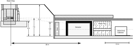
FIG. 1.: Detector enclosure and target area configuration, elevation view

The detector was located about $30{\,{\rm~{}m}}$ from the neutrino source and was shielded by the equivalent of $9{\,{\rm~{}m}}$ of steel. A schematic of the layout is shown in Fig. 1. The detector was under $\sim 2\,$kg/ cm² of overburden reducing the cosmic ray flux significantly from that at the surface. A liquid scintillator veto shield surrounded the detector on all sides except on the bottom. The detector was a tank filled with 167 metric tons of mineral oil (CH₂), with a small admixture (0.031 g/l) of butyl PBD scintillant. This dilute mixture allowed the detection of both $\check{\rm C}$erenkov light and isotropic scintillation light. This resulted in robust particle identification for $e^{\pm}$, location of the event vertex in space, and a measurement of the $e^{\pm}$ direction. The light was detected by 1220 8^′′ PMTs, covering $\sim 25\%$ of the surface inside the tank wall. Each channel was digitized for pulse height and time. The electronics and data acquisition systems were designed explicitly to detect and correlate events separated in time. This was necessary both for many neutrino induced reactions and for cosmic ray backgrounds. The behavior of the detector was calibrated using a large sample of “Michel” $e^{\pm}$ from the decays of stopped cosmic ray muons. These $e^{\pm}$ were in just the right energy range for the $\bar{\nu}_{\mu}\to\bar{\nu}_{e}$ search.

Even with this shielding, there remained a large background to the oscillation search due to cosmic rays, which needed to be suppressed by about nine orders of magnitude to reach a sensitivity limited by the neutrino source. The cosmic ray muon rate through the tank was $\sim 4$  kHz, of which $\sim 10\%$ stopped and decayed in the scintillator. Details of the suppression of this background in the DAR search will be discussed in reference [6]. Finally, any remaining cosmic ray background was very well measured because about 13 to 14 times as much data were collected when the beam was off as on. The result of these procedures was to reduce the cosmic ray background below the level of sensitivity required for the decay at rest oscillation search; similar techniques were found useful for the DIF oscillation search.

1.3  Outline of this paper

After the introduction, we present a description of the neutrino source used in the LSND experiment in chapter two. The detector hardware are described in chapter three and the data acquisition is in chapter four. Chapter five covers basic detector simulation. Chapter six covers event reconstruction and calibration of the detector.

2.  Neutrino Source

2.1  LAMPF

2.1.1  Accelerator description

The linear accelerator at Los Alamos used conventional ion sources for protons and for H^- ions. Ion sources provided particles for acceleration that were selected on a pulse-by-pulse basis. Protons passed through a transition section to a drift tube linear accelerator of Alvarez type operating at 201.25 MHz. Protons were accelerated in this section to 50 MeV and then injected directly into a side-coupled linac structure operating at 805 MHz for acceleration to a nominal energy of 800 MeV. The acceleration process was repeated at 120 Hz. During the course of this experiment, all cavities were operational in the linac structure. This ensured that the output proton beam kinetic energy of 800 MeV was constant to much better than 1%. The linac output beam was transported to a high intensity area shown in Fig. 2. The output beam energy has been measured in this configuration, and the results are discussed in section 2.3.

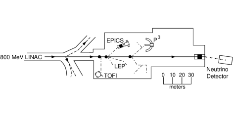
FIG. 2.: Schematic of the high intensity experimental area

2.1.2  Time structure of beam

The linear accelerator at times accelerated both proton and H^- beams in interleaved pulses. During much of the data taking in the period of the experiment, the proton beam was delivered at 120 Hz to the experimental area described below. For part of the run in 1993 and 1995, H^- beam at 20 Hz was delivered elsewhere and those pulses were not available to this experiment. Each of the 120-Hz proton pulses was approximately $600{~{}\mu s}$ long and had a substructure that consisted of pulses approximately 0.25 ns wide at 201.25 MHz.

The beam current at the output of the accelerator was typically 1 mA. The accelerating RF frequency was set for optimum beam acceleration in the linac and remained constant to parts in $10^{7}$ for the entire data taking period. The phase of the accelerated beam relative to the RF waveform was varied for optimum accelerator performance. The repetition rate was approximately synchronized to the line frequency so that long-term variation of this rate occurred at the level of 0.1% in a day. A beam permit signal (later referred to as H⁺) was generated preceeding acceleration and lasting through beam delivery. The gate that was generated by this signal was used after the fact to verify the relative timing of neutrino events and the accelerator cycle.

The existence of this beam permit signal was necessary for beam on-off subtraction. The amplitude of the beam typically varied by less than 1% over short periods, with overall beam availability in excess of 90%.

2.1.3  Upstream beam use

This experiment was performed at LAMPF where a broad-based program of nuclear science was carried out at the same time that the measurements of this experiment were being made. The program depended on secondary beams produced at two targets substantially upstream of the neutrino target A6. The two targets A1 and A2 were used to generate pion and muon beams for experimentation. Since pions were produced at these targets and subsequent decay occurred, they were also potential sources of neutrinos in LSND. Pions mostly decayed in the evacuated enclosures near these targets. The targets A1 and A2 were made of carbon, 3 and 4 ${\,{\rm cm}}$ thick, respectively. An estimate of the relative flux with respect to A6 for DAR was made by simply observing that the production rate was 25% of that at the neutrino target A6 and the distance was typically four times further from the neutrino detector. This gave a neutrino flux from this source of about 1.5% that from A6. The detailed calculation is discussed in sections 2.4 for DAR and 2.5 for DIF below.

2.2  Target geometry and shielding

Fig. 3 shows a plan view of the A6 target area and Fig. 4 shows an elevation view.

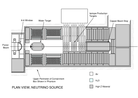
FIG. 3.: Plan view of the target box at area A6

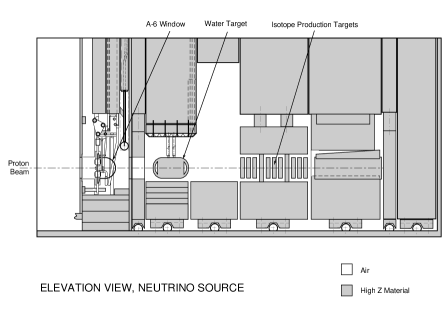
FIG. 4.: Elevation view of the target box at area A6

The proton beam entered from the left, passed through the water target and ended in the beam stop. The target consisted of an outer inconel vessel filled with water and fitted with baffles to direct flow. A larger scale diagram of the target used in ’94/’95 is shown in Fig. 5.

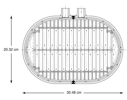
FIG. 5.: Construction schematic of the water target assembly used in ’94/’95

Rapid water flow, necessary to prevent boiling during beam passage, was monitored to verify target conditions. The ratio of mass of inconel to water was about 25% for the proton beam, which passed normally through the baffles; this ratio was slightly larger for secondary pions that were produced at finite angles. Water-cooled iron shielded the entire region. Within this shielding around and downstream of the target was a volume in which pion decay occurred. The shielding was hermetically sealed, partly because neutron background would be a serious problem if the shielding were not complete and partly because activation of the air near the target region would be a health hazard if the air were not contained. The DAR part of the experiment depended on suppression of the decay of negative muons, which was accomplished first by the fact that negative pions that stop were all absorbed. Those negative pions that decayed in flight before coming to rest produced negative muons that almost entirely stopped either in iron, copper or in water-cooling channels. Typically, 9% of $\mu^{-}$ stop in water, almost entirely in the production target. A typical pion had a momentum of 200 MeV/$c$ and $\beta{\gamma}c\tau$ = 12 m. This was long compared to a typical trajectory and resulted in a fraction of pions that decay in flight of about 3.4%. The inserts in Fig. 3 and 4 that are labelled “isotope production targets” were targets for producing radioisotopes and were responsible for a small amount of pion production, which was taken into account in the simulation of neutrino flux.

In Fig. 2 is shown two upstream targets A1 and A2, which were also included in the simulation of neutrino flux. Each of these targets was mounted in an enclosure which was surrounded closely by hermetic shielding except for vacuum pipes which permitted egress for four secondary beams, one on each side for both targets.

2.3  Characteristics of 1993, 1994 and 1995 Runs

The beam conditions in 1993, 1994 and 1995 were slightly different. In 1993 the target thickness at A1 was $3{\,{\rm cm}}$ and at A2 $2{\,{\rm cm}}$, both carbon targets of uniform thickness along the beam. In 1994 and 1995, A2 was increased to $4{\,{\rm cm}}$. The kinetic energy of protons from the linac was 797 MeV and was known to about 1 MeV. After the A1 target the beam emerged at 786.5 MeV and after A2 it was 767.6 MeV. The proton current loss was 85 $\mu$A at A1 and 103 $\mu$A at A2. These conditions were quite stable through the running period in 1994 and 1995. In 1993 the A2 target suffered some erosion of thickness, which was tracked and compensated. The neutrino water target was $20{\,{\rm cm}}$ in thickness in 1993, $30{\,{\rm cm}}$ in 1994 and 1995. This increase in thickness, together with the slightly lower energy due to the increase in A2 thickness in 1994, resulted in an increase in the DIF ${\nu_{\mu}}$ flux of 8%. The target was not in place for part of the time in 1995, which was accounted for in the total flux calculations. The charge delivered to the beam stop in 1993 was 1787 C, in 1994 it was 5904 C, in 1995 4794 C with target in and 2286 C with target out. Each of these charge accumulations was with the detector in operation and taking data.

2.4  Decay at Rest Neutrino Flux Calculation and Measurement

A detailed simulation was used to predict neutrino fluxes at the detector and is described in [4]. Measurements of pion production fluxes that were taken at a number of proton energies at LAMPF [7] were used as input to this simulation. The detailed geometry of the sources (A1, A2, and A6) described above were included in the simulation. In addition, the yield of muon decays was determined in a separate experiment [8] in which a proton beam of variable energy was introduced into a composite structure of water and copper to approximately duplicate the materials in which pion production occurred in this experiment. The overall number of muon decays per incident proton was determined in this subsidiary experiment, and the neutrino flux calculation was renormalized slightly to fit the measured yield in the separate experiment. It should be noted that this procedure normalized the neutrino yield from positive pions quite well, but since the negative pions were almost entirely absorbed, the measurement was insensitive to the consequences of the negative pion decay rate. The shape of the neutrino flux from $\pi^{+}$ and $\mu^{+}$ DAR is well known and is shown in Fig. 6, so that only the absolute amplitude was determined from experiment and simulation.

FIG. 6.: Flux shape of neutrinos from pion and muon decay at rest

The $\bar{\nu}_{\mu}$ flux integrated over energy for the configuration described here was $7.6\times 10^{-10}\ \bar{\nu}_{\mu}$ / cm²/proton averaged over the fiducial volume of the detector. The ${\nu_{e}}$ flux is identical to the $\bar{\nu}_{\mu}$ flux. The DAR simulation depended on the geometry at the three target stations in which substantial beam interacted. Beam loss in the accelerator and in locations other than target areas was very small because operational and health considerations made it imperative to lose very little of the proton beam in other than specially hardened areas. The targets at A1 and A2 were surrounded by enclosures that were typically $50{\,{\rm cm}}$ in dimension with closely packed steel shielding, apart from relatively small apertures for beams to emerge. The distance from A1 to A6 was 107 m and A2 to A6 was 82 m. The calculation of the DAR flux was then relatively simple, and the DAR spectra at the detector was governed by solid-angle considerations and the interaction fraction in the target. Pion DAR was isotropic and muon decay was effectively isotropic because spin precession and the varying production angle washed out angular effects. There was one exception to this, which is discussed in the next section: that part of pion production that occurred at small angles and thus was able to pass down the beam pipe for a significant distance. The “in-flight” decay probability was then much larger than in the target enclosures, and subsequent muon decay probability in flight was also enhanced. Detailed simulation gave a DAR flux at the detector from positive pion and muon decay that was 0.5% from A1, 1% from A2, and 98.5% from A6.

An additional corroboration exists from the experiment [9] performed at 90^∘ to the same target that measured neutrino-electron elastic scattering as a test of Standard Electroweak theory. This cross section of ${\nu_{e}}$ scattering from electrons is now well known and can be used to estimate the flux in contrast to the procedure of that previous experiment. This provided an independent confirmation of the flux estimate used here with an uncertainty of 18%.

2.5   Pion Decay in Flight Flux

2.5.1  ${\nu_{\mu}}$, $\bar{\nu}_{\mu}$ Flux calculation

The calculation of the neutrino flux (${\nu_{\mu}}$) from pion DIF at the A6 beam stop, A1 and A2, proceeded in a similar way to the calculation of the DAR flux. The same input data were used to calculate pion production normalized in the same way as the data in the previous section. The overall positive pion DAR flux was known to 7% as constrained by the simulation experiment described previously. The negative pion flux lacks this constraint. However, the same normalization factor was assumed to apply because it came mainly from the effects of thick target particle production of $\pi^{\pm}$ by protons. It was believed that the geometry of the decay volumes, including the neighborhood of A1 and A2, is well known from the constraints attendant in mechanical assembly. A lack of knowledge of the shape of the pion production spectrum folded into this geometry introduced some additional uncertainty. These uncertainties have been estimated to increase the systematic error on the DIF fluxes to 12% in absolute magnitude [10]. A significantly smaller point-to-point uncertainty may be expected in the spectrum. The ${\nu_{\mu}}$ spectrum shown in Fig. 7 was at the center of the detector for the three years described in this paper. The integrated flux over the detector for this period was $6.2\times 10^{12}$ ${\nu_{\mu}}$/ cm². Although the flux at the center of the detector is shown in the figures, the integrated flux used a calculation of flux throughout the tank. As was mentioned in section 2.3 the water target was retracted from the proton beam for part of the data taking in 1995. With the water target out the DIF flux was $3.6\times 10^{-11}$ $\nu_{\mu}/{\,{\rm cm}}^{2}$/proton.

FIG. 7.: Calculated DIF energy spectra for ${\nu_{\mu}}$ and $\bar{\nu}_{\mu}$ at the center of the detector

A similar calculation was performed for negative pions that decay in flight, leading to the $\bar{\nu}_{\mu}$ spectrum also shown in Fig. 7 and an integrated flux of $8.0\times 10^{11}\bar{\nu}_{\mu}$/ cm² averaged over the detector volume.

2.5.2  ${\nu_{e}}$ and $\bar{\nu}_{e}$ flux calculation

Electron neutrinos were produced (occasionally) from pion decay in flight followed by muon decay in flight. The rare branching mode $\pi^{+}\to e^{+}+\nu_{e}$ also contributed to the $\nu_{e}$ flux. These contributions have been calculated and are shown in Fig. 8.

FIG. 8.: The left two figures are ${\nu_{e}}$ and $\bar{\nu}_{e}$ flux at detector center from pion decay. The right two figures are similarly calculated ${\nu_{e}}$ and $\bar{\nu}_{e}$ fluxes from muon decay.

2.6  Decay at Rest $\bar{\nu}_{e}$ Flux

Negative muons were produced through the chain of negative pion production and decay in flight. This was followed almost always by either decay or absorbtion of the negative muon in the field of a nucleus. This decay process in this experiment occurred dominantly in Fe and Cu although a fraction (35%) of decays were in oxygen in the water of the pion production target and in the water cooling of the shield. A $\mu^{-}$ in the lowest atomic state in Fe was contained in a potential of $\sim 1.9$   MeV, which influenced the momentum distribution of the $\mu^{-}$. In turn, this momentum distribution affected the decay spectrum of the outgoing leptons. These effects have been calculated by a number of authors for the electron [11] but not for the neutrino spectrum. The actual capture rates are well described by theory, and the data in [12] have been used to estimate the $\bar{\nu}_{e}$ rate expected in the experiment. The fraction of produced $\mu^{-}$ that decay has been estimated at about 12%. The energy spectrum of $\bar{\nu}_{e}$ from this source is approximately $x^{2}(1-x)$, where $x$ is the ratio of neutrino energy to the end point energy of the spectrum (52.8${\,{\rm~{}MeV}}$). This spectrum is significantly softer than that expected from $\bar{\nu}_{\mu}$ to $\bar{\nu}_{e}$ oscillations, $x^{2}(3-2x)$. The overall yield from bound muon decay was subject to the same systematic error as the pion DIF flux.

3.  Detector Hardware

3.1  Detector, Veto, and Shielding

3.1.1  Detector description

The experimental detector was situated in the enclosure shown in Fig. 1. The detector proper was contained in a steel tank roughly cylindrical in shape, 8.3 m long internally, with a diameter of 5.7 m, as shown schematically in Fig. 9.

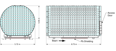
FIG. 9.: Schematic of the detector tank

The tank had a flat section on the top 1 m wide along the entire length where cable penetration into the tank occurred. The base of the tank was flat and rested on steel shielding extending along the full length and width of the tank. Type R1408 8 ^′′ Hamamatsu phototubes (PMTs) [13] were mounted uniformly on the walls with a mean photocathode coverage of 25%. This number was calculated as the total area of flat discs of the same diameter as the photocathode surface in the PMTs divided by the area of the tank walls scaled to the photocathode surface. The photocathode surface was approximately 25 ${\,{\rm cm}}$ inside the tank wall. Liquid entered the tank at the bottom closest to the target and an overflow outlet was situated at the top furthest end. Cables from the detector penetrated the tank at the top, passed outside the top of the tank toward the upstream end, and passed under the veto shield near the bottom front. In discussing the experimental geometry, the coordinate system that will be used is positive $z$ along the tank axis in the beam direction, $y$ vertical and positive up. The center of the coordinate system was at the geometrical center of the cylinder.

3.1.2  The veto shield

The detector was enclosed by a veto shield. This shield covered the entire detector apart from a support structure on the floor. It consisted of two parts, an upstream wall which was installed first and an approximately cylindrical part with a downstream wall which was rolled into place on rails after the detector was fully installed. This made the coverage of the shield as hermetic as possible. The shield had been built for a previous experiment [14] and had liquid scintillator as an outer layer with 12.5 ${\,{\rm cm}}$ of lead shielding inside the scintillator tank. A section of the veto shield is shown in Fig. 10.

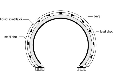
FIG. 10.: A cross section of the veto system through the x - y plane, roughly normal to the beam direction

The lead shielding absorbed neutral particles (photons and neutrons) which traversed the active veto before reaching the detector. Muons which stopped and decayed in the lead, producing Bremsstrahlung photons from electrons, were tagged by the active veto. The scintillator was viewed from the outside through portholes by a total of 292 5^′′ E.M.I. PMTs type 9870B. Twelve plastic scintillator counters (“crack counters”) were used to cover the optically weak region around the joint between the upstream veto wall and the veto cylinder. After the 1993 run, eighteen plastic scintillator counters (“bottom edge counters”) were added along the bottom edge of the veto counter to reject some of the cosmic rays that entered the detector from the sides near the floor.

3.1.3  Passive Shielding

The detector was situated 29.7 m from the production target under 2 kg/ cm² of steel overburden to shield from cosmic rays. This shielding was sufficiently thick to filter the hadronic component of cosmic rays but was penetrated by muons from cosmic-ray showers. These penetrating muons passed through the veto shield and detector and gave a rate in the detector of $\sim 4{\,{\rm~{}kHz}}$. Ten percent of these muons stopped in the detector and decayed, giving a source of electrons that was invaluable for calibration purposes. The detector was located in the veto shield inside a tunnel just large enough in diameter to contain the veto itself. A short portion of tunnel upstream of the detector was used for services and partial access to the detector and preamplifier electronics. Downstream, the detector was shielded by an 8 m long tank filled with water that also fitted in the tunnel closely as shown in Fig. 1. The detector rested on a concrete pad covered by six inch thick steel blocks. The cracks between these blocks were filled with steel shot. Upstream access was made through a 1m diameter labyrinth from the surface. Ventilation was accomplished through a second small-diameter tunnel that also had a labyrinthical character. Downstream of the beam stop, shielding equivalent to 9 m of steel attenuated the neutron flux produced in the beam interaction process. This resulted in a negligible neutron rate in the detector associated with the beam. This hermetically sealed structure provided excellent shielding both from cosmic rays and from beam-associated particles.

3.2  Liquid

The detector medium was designed to be sensitive to $\check{\rm C}$erenkov light from electrons and relativistic muons and scintillation light from all charged particles. A dilute mineral-oil-based scintillator was used to accomplish this. Mineral oil was well suited for this detector. It had radioactive contamination below a part in 10¹², it retained a stable attenuation length as it was not exposed to oxygen, it was non-toxic, had a high flash point (105^∘ C), and it had a high index of refraction of 1.47, implying a $\check{\rm C}$erenkov cone angle of 47.1^∘ for $\beta\sim 1$ particles. This high index of refraction increased the amount of $\check{\rm C}$erenkov light that was radiated by an electron by a factor of 1.57 compared to water. Chemically, mineral oil is composed of linear chain hydrocarbon molecules ($C_{n}~{}H_{2n+2}$) where $n$ varies from 22 to 26. Isotopically the carbon was 1.1% ¹³C and 98.9% ¹²C.

Extensive testing of various mineral-oil-based scintillators was performed in a beam containing positrons and protons in a test channel at LAMPF [15]. Angular distributions of the light emitted by relativistic and non-relativistic particles in this beam allowed optimization of the ratio of isotropic light to $\check{\rm C}$erenkov light. Typical angular distributions for water, pure mineral oil and the mixture that was used in this detector are shown in reference [15]. A concentration of about 0.031 g/l of b-PBD (butyl-phenyl-bipheny-oxydiazole, CHNO) in mineral oil was determined to be optimum for this detector. For a fast moving particle ($\beta=1$), the ratio of the number of photoelectrons generated from isotropic light to that from direct $\check{\rm C}$erenkov light was determined to be about 5 to 1. Isotropic light was emitted directly by the scintillator from particle ionization together with a contribution from ultraviolet $\check{\rm C}$erenkov light that was absorbed near the production point and then reemitted by the scintillator. A global fit to the sum of isotropic light and that in the $\check{\rm C}$erenkov cone was used for particle identification and to reconstruct vertex and angle information for relativistic particles.

Tests were also conducted to ensure that those components that were in direct contact with the b-PBD liquid scintillator, such as signal cables, PMT bases, and the interior black epoxy paint, did not contaminate the scintillator. Light attenuation measurements were periodically made at eight different wavelengths from 340 to 550 nm to monitor the ageing of scintillator maintained at elevated temperatures exposed to these components.

The oil that was used was Britol 6 NF HP White Mineral Oil [16]. The oil was delivered to the detector site in December 1992 and stored in a 52,000-gallon storage tank next to the neutrino tunnel. This tank was protected internally in the same way as the detector tank. After the PMTs were installed and the detector sealed, the oil was pumped from the storage tank into the detector through stainless steel plumbing in April 1993. The b-PBD scintillator was added to the mineral oil inside the detector over a two-week period in August 1993. A total of 6 kg of b-PBD powder was dissolved in approximately 50,000 gallons of oil. The final concentration of b-PBD was measured to be 0.031 g/l. During the time of storage and while inside the detector, air was excluded and the liquid was exposed to a pure nitrogen atmosphere. Samples of liquid scintillator taken from near the top and near the bottom of the detector after the 1994 period showed no difference in the concentration of b-PBD at these two extreme positions within the measured uncertainty of 5%.

Liquid inside the detector was kept at a constant temperature of $\sim 15^{\circ}$ C by a heat transfer unit. The density of the scintillator was measured to be 0.85 g/ cm³, giving a number density for carbon atoms of $n=3.63\times 10^{22}$  cm^-3. The ratios of other target atoms to carbon in the scintillator were $H/C=2.05$, $N/C=3\times 10^{-6}$, and $O/C=1.5\times 10^{-6}$. The attenuation length of the scintillator was monitored periodically during all running periods to determine changes that would indicate ageing or contamination. No deviation, within errors, from the starting attenuation lengths was observed at the eight wavelengths monitored. An attenuation length of about 20 m was characteristic of the scintillator at wavelengths of $\sim$400 nm near the peak quantum efficiency for the Hamamatsu PMTs. The variation of attenuation with wavelength is shown in section 5.2.

3.3  PMT system and preamplifiers

The PMTs that were used in the detector tank were all tested and calibrated after delivery from Hamamatsu. The tubes were built to a special contract using low radioactivity glass. Testing consisted of physical inspection, base attachment, testing under high voltage, calibration and potting. Each PMT with base was put in a light-tight enclosure equipped with a light pulser. The light pulser, located 10 inches from the PMT photocathode, consisted of two light sources, a green LED for charge tests, and an avalanche transistor for timing tests. First, the PMTs sat under voltage for 8 hours with the dark rate measured every minute. Then charge spectra were taken at two voltages close to the suggested operating voltage by the manufacturer. The final operating voltage was determined by interpolation for a gain of $\sim 4\times 10^{6}$. Then noise and signal rate were determined as a function of voltage to see if a satisfactory plateau existed. A typical pulse height distribution for single photoelectron illumination is shown in Fig. 11. All of the tubes used in the detector were required to have a definite peak-to-valley in the single photoelectron distribution as shown in the figure.

FIG. 11.: PMT pulse height distribution for a typical phototube at normal incidence. The light level is such that tubes produce less than one photoelectron on average

FIG. 12.: Distribution of peak to valley parameter for detector PMTs

A distribution of the peak to valley parameter for the tubes used in the detector is shown in Fig. 12.

After testing, the base portion of the PMTs was dipped in Hysol, a one-component urethane material, which was primarily designed for printed circuit board coating. Hysol PC18 had high dielectric strength, cured at room temperature, and was extremely abrasion and solvent resistant. A description of the veto PMTs can be found elsewhere [14]. The PMTs were powered through high-voltage cards that distributed to each PMT the correct high voltage that was determined in the testing process. These cards also provided control and monitoring of high voltage through a monoboard computer interface. Each PMT channel was nearly identical, consisting of a resistive base operated at a positive supply voltage of approximately 2000 V and stepped down to maintain appropriate voltages at the dynodes of the PMTs used in the detector. A single 100-ft-long RG-58 coaxial cable connected each PMT to the preamplifier and high voltage card, where the cable was terminated. At the preamplifier input, the signal of the PMT was separated from the supplied high voltage on this common cable. The preamplifier amplified the anode signal by a factor of twenty and drove 100 ft of RG-58 50$\Omega$ cable to remote electronics for charge and time digitization. At the input to the remote electronics after transmission through the preamplifier and 200’ of cable, a typical single photoelectron pulse had an amplitude of 25 mV and a $\sim 6ns$ rise time. After-pulsing and undershoot on this signal were minimal. Some additional characteristics of all the PMTs are shown in Table I.

TABLE I.: Main characteristics of PMTs

	detector	veto	crack-counters
type	HAMAMATSU R1408	EMI 9870B	HAMAMATSU R875
diameter (in)	8	5	2
voltage range (V)	1600-2300	710-1400	1100-1350
base$~{}R~{}$(M$\Omega$)	17	15	6.27
average I ($\mu$A)	110	70	190

3.4  Laser Calibration System

A $N_{2}$-dye laser calibration system was installed to calibrate both timing and amplitude response for each individual PMT channel. It consisted of a pulsed laser [17] located remotely from the detector. This laser was connected to three fiber-optic cables which channeled light to three glass bulbs $10{\,{\rm cm}}$ in diameter. The 337 nm output wavelength was shifted by a Coumarin dye cell to 420 - 40 nm. The time spread of the light was less than $\sim 1ns$ rms, short compared to the system response. The coordinates of the flasks are given in Table II. These glass bulbs were filled with Ludox [18] as a dispersant. The feedthrough bringing the light pulse into a flask entered from the top and terminated 2 ${\,{\rm cm}}$ short of the center. The light amplitude was varied through remotely controlled attenuators prior to the fibers. The average light level was varied so that all channels of the detector were calibrated over the full response range. Each bulb was activated independently and remotely. The state of the pulsing system was recorded by the data acquisition system. The positions of the bulbs were known from a survey and remained fixed through the course of the experiment.

TABLE II.: Coordinates of Ludox bulbs

Flask	x (${\,{\rm cm}}$)	y (${\,{\rm cm}}$)	z (${\,{\rm cm}}$)
1	-36.5	27.3	-143.5
2	35.2	28.6	1.3
3	-35.2	27.9	221.6

3.5  Beam Timing Signals

Data acquisition operated independently of the state of the beam. This knowledge was available to off-line analysis, however, in two ways. A prepulse was delivered from accelerator control that was used to start a timer in data acquisition that allowed the time for each event to be recorded with respect to this starting time. Additionally, a level was also available that was recorded whenever beam was present. The mechanics of the recording process are discussed in the data acquisition section below.

The fine time structure of the beam was determined by the RF structure present in the 201 MHz part of the linac described in section 2. The proton beam consisted of bunches approximately 5 ns apart (4.969) with a width of about 200 ps rms. Upstream of the experimental area shown in Fig. 2 were pickup plates designed to provide a signal induced by the passage of the proton beam. This signal consisted of pulses one nanosecond wide at the bunch frequency 201.25 MHz. The amplitude of these signals was proportional to individual beam bunch size, but because the beam was quite stable it proved sufficent to measure beam arrival time with a single level discriminator. This discriminator output was transmitted through a fiber optic link to the remote electronics station. At the data acquisition electronics the signal was counted down by a factor of eight and then sixteen parallel signals were generated, each of which repeated after 640 ns. Each of these signals was sent to a specially modifed digitizing channel capable of dealing with this repetition rate at the input. For any event, therefore, a number of measurements of beam arrival time was available with each channel offset by $\sim$ 40 ns from its neighbour. These measurements of beam arrival time were used to calculate the beam arrival time relative to an event. Knowledge of the arrival time of proton bunches was desirable for those parts of the experiment that used pion DIF generated neutrinos. In the study of DIF events and ${\nu_{\mu}}$C events in particular, this information was used to identify events which maintained a time correlation with the proton beam. The details of the data analysis method will be described in the subsequent publications where these data were important.

4.  Data Acquisition and Calibration

4.1  Overview and Architecture

Data were acquired by this detector on the basis of energy deposition in a short time period. This data acquisition system was designed to detect a primary trigger with energy deposition in excess of approximately 4${\,{\rm~{}MeV}}$ electron equivalent and then to acquire data nearby in time with a different energy threshold. In Fig. 13 is shown a schematic of a single PMT channel.

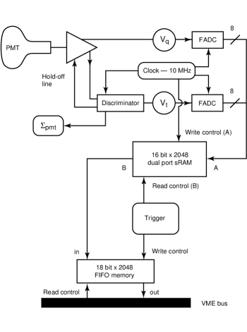
FIG. 13.: Single channel block diagram

The electronic digitizing system was designed to collect charge from each PMT, digitize time and amplitude, store these data for a substantial period and generate a trigger for data retrieval. This task was accomplished in the presence of a significant counting rate from cosmic rays and ambient radioactivity. A ‘hit’ in a channel corresponded to a minimum pulse height of $\sim 1/4$ of the peak response to a single photoelectron in an average-gain PMT. Neutrino induced events consisted of primary events containing more than 100 hit tubes pulsing within 200 ns of each other, followed in time by secondary events containing 21 to 200 hit tubes. Secondary events occurred on timescales varying from a few hundred ${~{}\mu s}$ for neutron capture to tens of milliseconds for nuclear $\beta$ decay. The individual dark pulse rates of the PMTs ranged from 1 to 5 kHz, producing a noise background that the acquisition system dealt with without affecting the trigger.

The experiment ran off a local binary 10 MHz clock which was synchronized to a global positioning system [19]. Each channel had pulse height and fine time digitized by flash ADC [20] every 100 ns in synchronism with this clock. These data were then stored in random access memory (RAM) in each channel at a common address, given by the least significant 11 bits of the clock. Each channel RAM contained a $204.8{~{}\mu s}$ history of activity in that channel. A count of hit channels was updated at each 100ns clock tick for both the detector and veto systems and these sums were used to initiate a primary trigger and secondary activities. After the trigger readout order was broadcast to each channel, data were transferred to a FIFO buffer at each channel, and data common to the event were stored in a trigger FIFO memory. This memory was interrogated by a master monoboard for the next level trigger generation. After data were transferred to channel FIFO, events were assembled at the crate level by a local monoboard [21] in each crate and on completion sent to the SGI multiprocessor system [22] for event building and reconstruction. The trigger operated independently of the state of the LAMPF beam, and tagged individual events as in-time or out-of-time with the LAMPF proton macropulse. The beam-unassociated background to any neutrino signature was determined by counting its occurrence in the beam-off sample and scaling by the beam-on/beam-off ratio of $\sim 0.07$. The determination of this factor is discussed in chapter six.

In the following sections some terms will be used which we define here. A “primary event” was one which satisfied a threshold of $\sim 100$ hit tubes in the detector and had no veto signal either nearby in time or in the previous $15.2{~{}\mu s}$. An “activity” exceeded one of the detector thresholds without meeting the requirements for being a “primary”. A “timestamp” was the time of a digitization as measured by the “binary clock” and also the address in channel memory where the “fine time” and “charge” were recorded for each channel. “QT cards” housed digitizing channels for “fine time” and “charge”. Data were recorded either for a “primary” or an “activity” after a “timestamp” was “broadcast” from the trigger system to “receivers” in each QT crate.

Memory pointers in each channel RAM were set to the same location, with the address described by the least significant 11 bits of the 10MHz binary clock. First level triggers were generated from an instantaneous global count for either the detector or the veto shield. This trigger produced a transfer from channel RAM to a FIFO attached to a particular channel and a latched summary data word into trigger memory. In parallel with this process, an event header was generated for transmission to the multiprocessor event handling system described in section 4.4.

4.2  Electronics

4.2.1  Digitizing System

In each QT card, charge and time-of-arrival information were digitized and stored. The least significant eleven bits of the GPS based clock were distributed to all modules generating times at which flash analog-to-digital converters [20] sampled data. This binary number was also the address in RAM at which digitized data were stored identically in each QT channel. The clock was distributed from a central driver so as to arrive synchronously at each QT card within a few nanoseconds. This clock determined a coarse time of arrival for PMT signals which was, as stated above, numerically the same as the address in the 2048 deep local channel dual-ported RAM. A fine arrival time for a PMT anode pulse was determined by a leading edge comparator set to the hit threshold defined in section 4.1. The comparator signal started a linear ramp that rose for two subsequent “clock ticks,” after which the ramp was reset to zero before the next 100 ns clock tick arrived. Once inititated, this timing ramp was unaffected by subsequent photoelectrons for 200 to 300 ns depending on the phase of the initial hit with respect to the 10 MHz clock.

The ramp voltage was flash digitized at each clock tick by an 8-bit FADC [20] and stored in a dual-ported RAM attached to this channel. The “fine time” determined this way had a least count of 0.8 ns. The anode pulse was also connected to an integrator-stretcher that convoluted it with an exponential with a decay time constant of 700 ns (6000ns in 1993). The stretched pulse was digitized by another 8-bit FADC at each clock tick, and digital output was sent to a parallel dual-ported RAM, as part of a 32 bit word at the identical address to the fine time. Again, all the address counters controlling FADCs and dual-ported RAMs were synchronized by the 100-ns clock. At the start of each cycle through memory locations in the RAM, the addresses of all RAMs were reset to zero to assure long term synchronization of the data in memory. The FADC-dual-port-RAM circuit operated continuously, filling channel memory with the time history of that PMT. “Latency” will be used to describe the case in which events were retrieved after memory was overwritten and hence contained irrelevant data. The small loss of data from this effect is described below in section 4.3. After a trigger decision was made (described in section 4.3), data were transferred from appropriate addresses to a FIFO. Interrogation took place through the second RAM port. Data resided in this FIFO buffer until it was read out by a dedicated monoboard computer [21] servicing 16 QT cards, i.e. 128 channels.

A schematic illustration of the system layout is shown in Fig. 14.

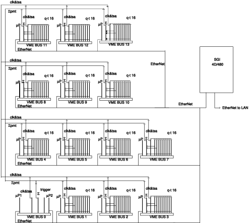
FIG. 14.: Schematic of data acquisition system electronics

The pulse digitization system described above was built in VME format using 9-U by 380-mm cards. This system was housed in 13 VME crates, each crate packed with 16 QT cards of eight channels per card. In addition, each crate housed a receiver-trigger interface card, a crate channel summation card, and a MVME167/D1 monoboard computer. The receiver-trigger interface card was driven by the trigger system described below and initiated data transfer to FIFO after receipt of a trigger broadcast.

4.2.2  Channel Sum System

Trigger input information was derived from a majority summation system. Each channel discriminator in a QT card generated a logic signal which was asserted at the next clock tick after an anode pulse arrived, and remained asserted for two clock ticks. These logic signals were summed digitally at the crate level. Appropriate crates were then summed digitally for both 1220 detector and 292 shield PMT signals to make an 11-bit detector sum and a 9-bit shield sum in the central trigger crate. These sums were available as binary signals representing a channel count of those that fired in the last two clock intervals. The count was updated every clock cycle. Each binary number, detector and veto, was fed to digital comparators that produced output if the sum was greater than or equal to values preset in hardware. Supplemental veto counters (“crack counters”) each generated a trigger condition equivalent to the firing of six or more veto tubes. These comparator signals were used as the basis of trigger decisions described in section 4.3. Trigger algorithms and internal operation of the trigger system are also described in section 4.3.

4.2.3  Performance Differences in 1993, and 1994/1995

There were several significant differences in data acquisition between data in 1993 and 1994/95. The transfer function in the amplitude channel of each QT card was non-linear at low pulse heights in ’93. The gain of each channel was also somewhat different. Full-scale for 1993 corresponded to $\approx 24$ times the peak of the single photoelectron response (Fig. 12 for an average-gain PMT, vs. $\approx 30$ times for 1994/95. In 1993, the lowest 4 ADC counts spanned $\sim 3$ times the charge that would be expected for a linear convertor. In ’94 changes were introduced that made the transfer function linear up to the top of the ADC range. In ’93 the integration time constant for time digitization recovery was $6{~{}\mu s}$; in ’94/’95 this was changed to $0.7{~{}\mu s}$. In both cases the effective transfer function was equalized in higher level software leading to very similar detector properties in each channel. After correction, a small degradation of resolution remained due to the large charge spread for low ADC counts.

TABLE III.: Table of tank hit D and veto hit V requirements for various trigger types for 1993 through 1995 running periods. Betas generate a single trigger broadcast. Primaries add the broadcast of all Activities within the previous 52.8 $\mu$sec. In addition, some Primaries cause the broadcast of all Gammas within the following 1 ms, and some generate the six $\mu$sec lookback.

1993	1994 early	1994 late	1995	Function
$D\geq 18orV\geq 6$	$D\geq 18orV\geq 6$	$D\geq 18orV\geq 6$	$D\geq 18orV\geq 6$	Activity
$D\geq 21andV<6$	$D\geq 21andV<4$	$D\geq 21andV<4$	$D\geq 21andV<4$	$\gamma$
none	none	none	$D\geq 75orV<4$	$\beta$
$D\geq 100andV<6$	$D\geq 100andV<4$	$D\geq 125andV<4$	$D\geq 150andV<4$	Primary
$D\geq 300andV<6$	$D\geq 100andV<4$	$D\geq 125andV<4$	$D\geq 150andV<4$	Primary, $\gamma$ window
none	none	none	$D\geq 300andV<4$	Primary, $\gamma$, lookback

4.3  Trigger

4.3.1  System Hardware

The information on which trigger decisions were based was an updating sum of hit tubes described in section 4.2.2. Trigger electronics and monoboards were housed in a single 6U crate. A block diagram of this system is shown in Fig. 15.

FIG. 15.: Trigger system hardware schematic

The modules consisted of a global digital sum card, comparator and logic memory FIFO card, two monoboards which were referred to as master and satellite, and a broadcast card. The detector and veto shield global digital sum cards referred to in section 4.2 completed the global sums that were used in the trigger.

These sums were interrogated by a comparator system which set levels when global sums exceeded preset values. These values are referred to as $D_{n}$ for the detector and $V_{n}$ for the veto. In Table III is shown the comparator level settings for each period of data taking. The primary threshold was raised in the middle of the 1994 run, and this is indicated in Table III. After a primary or activity comparator level was set, data describing the event were written to a trigger memory FIFO. These data included the full 16 bit binary clock time, the state of the comparator bits and four external data lines describing laser status, beam gate, bottom edge veto counters and prebeam timing signal. The trigger master monoboard polled this FIFO and, whenever data were present, subjected FIFO data to conditions for primary event selection and for activities nearby in time, both of which are described in the software section below. On receipt of a completed event, header information was assembled by the satellite monoboards, and event addresses were broadcast to receiver cards located in those 13 crates that housed QT cards. This occurred when the master monoboard loaded a register in the broadcast card with the timestamp. After receipt of this timestamp in the receiver cards, transfer from channel RAM to FIFO occurred. Presence of a data present signal in channel FIFO prompted each QT crate monoboard to transfer six contiguous locations in each FIFO to memory. This process continued until all channel FIFOs were empty. On completion, these assembled event components were transferred to the SGI multiprocessor system through an ethernet link of all system monoboards described in section 4.4.

FIG. 16.: Flow diagram, master monoboard software

4.3.2  Software Selection

A flow diagram for event selection in the master monoboard is shown in Fig. 16. Input data for this process were contained in the trigger memory FIFO and in a circular buffer, maintained in master monoboard memory, of all activities that asserted an appropriate D or V level. This activity data included the binary time of occurrence and comparator levels in veto or detector. After each of the checks described below, the activity found in trigger memory was added to the activity stack in the master monoboard buffer. The first loop in Fig. 16 checked for veto activity and updated the record of the time of the previous veto event. If there was no veto activity, a check was made for veto activity in the previous $15.2{~{}\mu s}$. If neither of these were true and the detector primary level was asserted, the event was accepted as a primary trigger. A broadcast was then initiated and QT data moved to channel FIFO. If a primary trigger remained asserted after six clock ticks then a broadcast was initiated for the next six. This often happened after a trigger from a high energy cosmic ray event made enough late scintillation light. Each six ticks, with five intervals was referred to as a “molecule”. If in addition the detector threshold was met, a ${\gamma}$ flag was set. If the ${\gamma}$ flag was asserted an activity in the subsequent millisecond was classified as a ${\gamma}$ candidate.

In summary, primary triggers were determined mainly by a threshold in the detector but with restrictions from the veto shield. After a primary, a lower threshold was used to initiate broadcasts as ${\gamma}$ candidates. When the event was passed on to the next level, up to four activities closest in time to the primary in the $51.2{~{}\mu s}$  previous to the event were broadcast as well as all ${\gamma}$ candidates in the succeeding 1 ms. The 100-tube trigger corresponded to $\sim 4{\,{\rm~{}MeV}}$ in electron energy and the 21-tube trigger to $\sim 0.7{\,{\rm~{}MeV}}$ in ${\gamma}$ energy. A $\beta$ trigger generated a single trigger broadcast. In 1995, a primary level with $\gamma$ was used to “look back” at the ${6\,\mu{\rm s}}$ prior to the primary, by generating two broadcasts to cover that period.

4.3.3  Trigger Rates

As was described above, the basic data rate of the system was the 10MHz clock driving digitization rates. The synchronous discriminator in each data channel fired at an average rate of 5${\,{\rm~{}kHz}}$, reflecting the sum of anode pulse rates in each channel from dark current and physical processes in the detector. The mode of the dark current rate in the ensemble of PMTs was 2${\,{\rm~{}kHz}}$. The remaining rate was dominated by cosmic ray muons and was 4${\,{\rm~{}kHz}}$ under the overburden of the detector. Either D or V was asserted at a total rate of $\sim 17{\,{\rm~{}kHz}}$, prompting address data transfer into the trigger memory FIFO.“Primary event” identification by the master trigger monoboard produced a rate of 20${\,{\rm~{}Hz}}$. Each of these primaries on average had associated activities that raised the data rate to $\sim 40{\,{\rm~{}Hz}}$, which was the rate of broadcasts to QT crates for data accumulation at crate level. This trigger rate of $\sim 40{\,{\rm~{}Hz}}$ was dominated by a few beam-unrelated processes. Beam-related neutrino interactions occurred at a rate of only about one per hour, which is down by a factor of $\sim 10^{-5}$ compared to the beam-off background. Fig. 17 shows the raw PMT multiplicity distribution for all broadcast events.

FIG. 17.: Raw PMT multiplicity distributions for all broadcast events

The high end of the spectrum, where almost every PMT was hit, corresponded to through-going cosmic muons. The region below the peak, from 650-1050 hit PMTs, was dominated by a combination of cosmic-ray muons and neutrons. Michel electrons from cosmic muons that stopped and decayed in the detector occurred in the 250–650 hit PMT region and were greatly reduced by disabling the trigger for $15.2{~{}\mu s}$ following activity in the veto shield. Finally, electrons from ¹²B $\beta$ decay, produced dominantly by cosmic-ray $\mu^{-}$ that captured on ¹²C, typically had 100-250 hit PMTs while radioactive ${\gamma}$ (e.g., from Th, K, and Co decay) have $<100$ hit PMTs. There is a sharp edge at 100 hit PMTs in Fig. 17 because the $D_{3}$ level is set to 100 for these data. Of the total rate, approximately 10${\,{\rm~{}Hz}}$ were beta decays of ¹²B from muon capture, 10${\,{\rm~{}Hz}}$ from natural radioactivity in the PMT glass and surrounding material, 0.11${\,{\rm~{}Hz}}$ from decay electrons from stopped cosmic ray muons, 1${\,{\rm~{}Hz}}$ from muons that evaded the veto shield and crack counters and 1${\,{\rm~{}Hz}}$ from neutrons produced from muons that did not enter the detector. These were the rates of primary triggers; associated activities contributed a similar rate.

4.3.4  Latency, FIFO Half Full Inhibit and Trigger Efficiency

Data taking rates in the detector were quite constant because they were completely dominated by cosmic rays and natural radioactivity. The trigger rate was adjusted to an acceptable level at the start of data taking by varying the settings of the D_n comparators for primary threshold and for activities. Occasionally, fluctuations in these rates caused the channel FIFOs to fill up, and when the half full flag was asserted in any FIFO the trigger was inhibited until the situation was cleared by data acquisition. This occurred $<1\%$ of the time. Similarly, the master trigger monoboard occasionally took long enough to process an event that channel RAM was overwritten, a condition referred to as latency. The loss of data from latency was $\approx 1\%$. These losses remained approximately constant throughout data taking as might be expected from the primary sources of data in the detector. One source of these conditions occurred when the SGI multiprocessor did not remove data from crate monoboards, whereupon channel FIFOs were not emptied and the acquisition part of the system was halted. This effect was included in the FIFO half full estimate and is the major source of this condition.

4.4  Data Readout and Event Building

4.4.1  Raw Data

The primary trigger caused data to be transferred from channel dual-port RAM to channel FIFO in sets of six timestamps. This corresponded to a time window of $0.5{~{}\mu s}$. Each crate monoboard running asynchronously was set up to poll all FIFOs in the crate to determine if data were present and if so, raw data were transferred to monoboard memory. Two bytes per timestamp (one each for time and charge digitizers) were read out for each channel in a crate. For a full crate of 128 channels, 1536 bytes of raw data were read out over VME for a six timestamp event. In each crate monoboard, a 32-bit header was constructed by interrogating the crate receiver card. This header included 11 bits of timestamp address (TSA) and an 8 bit counter to assure FIFO synchronization.

4.4.2  Compact Data

Compact data were formed in the QT monoboards from raw data. Information was reported from six sequential TSAs covering five time intervals for hit tubes in the crate. Longer events were handled in a slightly more complex way, but the essential point was that six timestamp molecules formed the basis for data transmission. Each compact data block was made up of a header followed by channel data for tubes that were hit. The compact data header included information which allowed the event builder to verify proper assembly of event fragments. Channel data consisted of a 16-bit header, followed by 8 bits for each interval with fine time and 8 bits for each charge deposition. After an interval with fine time information, the QT hardware did not provide fine time information for the next two intervals, but charge increments were still registered. Baseline amplitude was the amplitude before pulse height digitization and was used for baseline subtraction. An interval stored with fine time was termed a “hit with fine time”. If no fine time was available it was called a “hit without fine time”.

In each crate monoboard, data were searched for hit PMTs by looking for rise and fall of the timing ramp as a function of time as signature. The difference between the baseline and maximum value of timing ramp was stored for later determination of fine time. For a hit occurring between TSA n and n + 1, fine time information was stored as ADCt(n + 2) - ADCt(n). In the last interval, however, fine time was calculated using a default value for the timing slope. To first order, the PMT charge $V_{q}$ in a given interval was simply the difference between ADC measurements before and after that interval. This was complicated by 3 effects: (1) $V_{q}$ required at least 30 ns to attain maximum value; (2) $V_{q}$ was slew-limited at 2.2 ADC channels per ns (this was only relevant for hits over 66 ADC counts); (3) $V_{q}$ decayed to its original baseline voltage approximately as an exponential with $\tau$ = 755 ns (6000ns in 1993). These effects were taken into account in computing the charge for each hit, using a linear approximation to the exponential effect (3). Except for 1993 data, additional charge increments occuring close enough in time to a hit with fine time were ascribed to effects (1) and (2), and included with that hit. If the charge ADC was set to full scale immediately before a hit, the overshoot bit was set in the “baseline” variable for that PMT channel. The remaining 5 bits of the baseline were set to the 5 most significant bits of the ADC. These bits allowed a determination of ADC saturation.

4.4.3  Event Building and Calibrated Data

PMT data were transferred to a multiprocessor system [22] over two independent ethernet segments. Both raw and compact data were transferred to check integrity of compact data, but during the operation of the experiment raw data were prescaled to avoid acquisition induced dead time. In the multiprocessor, individual timestamp molecules from each crate were ordered by the CODA [23] package. Complete events were then built using data from the first four time stamps in each molecule. Apart from 1993 data, when these events were being built, the time information was converted to times relative to the first timestamp of the event; and each PMT time and charge was calibrated using constants determined from laser events, as described in section 4.6. The SGI multiprocessor contained 8 independent processors. Events were built in one processor, a second distributed events to the remaining six processors that were used exclusively for event reconstruction on line. The output of event building was the Calibrated Data bank in ZEBRA format, which served as primary input to the analysis package used both online and offline [24] . A header included a calibration data file identifier, number of timestamps in the event, and a hit count with and without fine time. This header was followed by tube number, charge and time and saturation for each hit.

4.5  Corrections for Digitizer Charge Response, 1993

For ’93 data, the Q circuitry had a $6{~{}\mu s}$ decay constant, and effects (1) and (2) above were not taken into account by the online software. The result was that in the ’93 data most hits were accompanied by hits without fine time in the subsequent interval. This effect was dealt with offline by adding the charge from these subsequent hits into the charge for the first hit. Another effect unique to the ’93 data was a nonlinear relationship between PMT charge and ADC value (especially noticable at low charge levels). This problem was also dealt with offline using a nonlinear mapping to recover PMT charge. After the ’93 run the nonlinearity was removed by a hardware upgrade. The quality of the 1993 data was high after correction. For example, the energy resolution deduced from Michel electrons was as good in 1993 as in 1994 and 1995.

4.6  Laser Calibration

Individual channel calibration was performed using the pulsed laser system described in section 3.4. A laser induced event was subjected to the same requirements ($>100$ hit tubes) as for any primary trigger. However, each event was identified by a set bit in fixed data in trigger memory. The laser system was pulsed at $\sim 0.1{\,{\rm~{}Hz}}$ continuously and asynchronously with the accelerator during normal data taking and at 20–30 ${\,{\rm~{}Hz}}$ during beam off periods for special purpose runs. This operation induced a negligible dead time, while providing a stroboscopic probing of the detector at times that were random with respect to beam arrival. The laser pulse time was tagged as a special event by the data acquisition system. Gain calibration was obtained from low light intensity runs by fitting the resolved single photoelectron peak for each PMT individually. Calibrations were performed periodically during the runs and have shown that calibration constants remained stable throughout the data-taking period. This low level of illumination was not adequate to provide timing calibration, so special data runs were interspersed at high light levels to provide timing offsets for all channels. Time-offsets of each channel were calculated individually from these high-intensity runs alone. Time-slewing effects were assumed to be identical for all PMTs, and a mean effect was calculated using laser data from all tubes, resulting in times calibrated to $\sim 1$ ns for each PMT channel.

5.  Detector Simulation

A detailed Monte Carlo simulation, LSNDMC[25], was written to simulate events in the detector using GEANT. The goal of the simulation was a complete description of events in the detector. For the decay-at-rest analysis, data from Michel decays of stopped muons and from captured cosmic ray neutrons were used to calibrate directly the response of the tank to the positrons and photons of interest. The simulation was used in this analysis to test understanding of the detector, particularly physical processes in the tank, reconstruction algorithms, and the computation of backgrounds. For the DIF ${\nu_{\mu}}$ to ${\nu_{e}}$ oscillation analysis, with higher energy electrons, the simulation was additionally used to find the efficiencies of analysis cuts. This implies greater sensiivity of the results to simulation details. This chapter focuses on issues of importance for the DAR analysis, and on using the simulation to understand physics processes occurring inside the tank. Some comparisons to Michel data will be presented in section 6.3.

5.1  Monte Carlo Ingredients

The GEANT geometry was defined to include the main detector tank, veto shield, and overburden for detector shielding. The latter two portions were implemented in order to track cosmic ray muons. Tank PMTs were positioned with a regular spacing, and within a few ${\,{\rm cm}}$ of the actual detector locations. They were represented as having hemispherical photocathodes, although when a computation of optical reflection probabilities was needed, an ellipsoidal shape could be substituted.

The Monte Carlo package included a variety of generator options [25]. Cosmic ray muons were generated with energy and angle distributions appropriate for the altitude of LSND. Among the variety of generator options included in the Monte carlo package [25] was a cosmic ray facility. Each muon was tracked through the overburden and veto shield, and so a set of starting locations for the generation of decay (Michel) $e^{\pm}$ was obtained. This allowed data vs. Monte Carlo comparisons. Also, estimates of the total muon rate in the tank ($\sim 4{\,{\rm~{}kHz}}$) and the stopped muon rate ($\sim 0.35{\,{\rm~{}kHz}}$) were in rough agreement with observations.

This simulation is addressed in detail in the following section. $\check{\rm C}$erenkov and scintillation light were simulated in detail, and each optical photon was tracked until it was either absorbed or generated a photoelectron. The PMT response to this photoelectron was also simulated. This set of steps resulted in one “hit”, in the GEANT sense, per photoelectron.

The digitization electronics and the online data acquisition algorithms were simulated using the full set of hits, yielding a time and an amplitude for each hit PMT. The hit time was simulated by using PMT pulse shapes determined from bench tests and laser data; pulses for multiple photoelectrons in the same tube were summed. The amplitude simulation used so far was based upon the 1993 version of both the QT digitizer cards and data acquisition algorithms, including the non-linear digitizer charge response. This non linearity was taken out in calibration. Both the simulation and the calibration of this response were based on bench measurements. Because the quantization imposed by digitization occurred for the non-linear amplitude, the 1993 data vs. Monte Carlo comparison was a more stringent test than the same comparison for 1994/95 data using QT cards that were linear. The digitizer time response depended upon details of pulse shapes, thresholds and fluctuations, and had a noticeable impact upon the way reconstruction algorithms worked. The discriminator in each channel produced a dead time after firing that inhibited measurements of subsequent photoelectrons. This effect was simulated in detail since it had a significant effect on actual event timing distributions.

5.2  Simulation of Photoelectron Production in the Tank

The basic physical mechanisms which occurred in the LSND medium and which contributed to a detected signal were scintillation from ionization energy deposits by charged particles and $\check{\rm C}$erenkov radiation by charged particles with $\beta>1/1.47$, including a contribution from $\delta$ rays. Optical photons from these processes were transmitted through the medium, taking into account absorption with or without fluorescent reemission. Photons could be reflected from the upper surface of the liquid or at the PMT surface. Photoelectron emission occurred at a photocathode and the spread from the multiplication process internal to a PMT was also simulated. Charged particles in the medium were tracked using GEANT, including particle interactions and full electromagnetic showers down to cutoff kinetic energies of $10{\,{\rm~{}keV}}$ for $e^{\pm}$’s and ${\gamma}$s. In order to simulate the contribution of $\check{\rm C}$erenkov radiation from $\delta$ rays, a minimum $\delta$ ray kinetic energy of $180{\,{\rm~{}keV}}$ was used. Delta rays contributed several percent of the total light from an electron event.

As GEANT stepped particles through the detector, it provided an energy loss $\Delta E$ to ionization for each step $\Delta x$. In the LSND simulation the mean number of scintillation photons was computed from Birk’s law [26]:

$${\bar{N}}_{s}={A\,\Delta E\over 1+k_{B}\,\Delta E/\Delta x}\ \ \ ,$$

where $k_{B}$ is a saturation parameter, discussed below. For particles with $\beta$ above the $\check{\rm C}$erenkov threshold (1/1.47), the mean number of $\check{\rm C}$erenkov photons in a given range of wavelength was computed by the formula in reference [27].

There are unfortunately no published measurements of $k_{B}$ for mineral oil scintillators. In the simulation we have used a value of 0.017 ${\,{\rm cm}}/MeV$, based upon typical measurements (scaled by density) for anthracene and several plastic scintillators [28]. However, other data give varied results, and there is some evidence based on limited measurements done for mineral oil by the LSND collaboration that the value could be as much as a factor of two smaller. We regard $k_{B}$ as uncertain at this level. This uncertainty has no effect on the response of the scintillator to electrons of interest, but is quite relevant for protons, especially for recoil protons in charged current neutrino interactions, for which the $\Delta E/\Delta x$ term in the denominator can dominate. For the lowest energy muons detectable as activities from $\nu_{\mu}+C$ interactions, the resulting change in light yield (and hence in energy scale) can be as much as 20%.

The absorption and emission properties of the dilute solution of b-PBD in mineral oil were key ingredients in modelling the behavior of the detector. b-PBD emitted light almost entirely at visible wavelengths ($\lambda>350{\,{\rm~{}nm}}$), with a sharp cutoff at shorter wavelengths[15]. The attenuation length for a sample of the mineral oil used in the tank was measured to be in excess of 15 m for visible wavelengths, falling to $<1\,$m for $\lambda<335{\,{\rm~{}nm}}$ as shown in [15] and discussed in section 3.2. Most of the scintillation light reached a photocathode or edge of the tank without absorption. The same was true for $\check{\rm C}$erenkov light emitted at visible wavelengths, which thus retained directionality. $\check{\rm C}$erenkov light emitted in the UV, however, was absorbed in a short distance. Light absorbed in the mineral oil was lost, but that absorbed by the b-PBD was reemitted isotropically via fluorescence with a probability of 0.83 and with an emission spectrum that was the same as for scintillation light. Hence for particles above $\check{\rm C}$erenkov threshold, a substantial part of the isotropic light was actually “converted” $\check{\rm C}$erenkov light. This Monte Carlo simulation included mineral oil and b-PBD absorption separately, so that the interplay of their absorption probabilities was properly taken into account at all wavelengths. The combined absorbtion length for light that is not reemitted as a function of wavelength for the LSND scintillator mix is shown in Fig. 18. $\check{\rm C}$erenkov photons were not tracked below $\lambda<350{\,{\rm~{}nm}}$ but were either absorbed or converted immediately.

FIG. 18.: Attenuation length for light that is absorbed without reemission as a function of wavelength for the LSND scintillator mix

There were three components to the produced light in the tank: direct scintillation light, directional $\check{\rm C}$erenkov light, and converted $\check{\rm C}$erenkov light. The latter two components were computed with no free parameters. To obtain the normalization constant $A$ for direct scintillation light, measurements were performed in a test beam using the same type of scintillator as was used in the LSND detector but with different phototubes [15]. In the test beam a measurement was made of the ratio of light in the $\check{\rm C}$erenkov cone to isotropic light for $\beta\approx 1$ positrons. This ratio was corrected back to the production point by correcting for relative PMT response and attenuation for the two types of light. Additional adjustments were made to conform to the precise definitions of the three components and for a slightly different b-PBD concentration in the detector from the test beam. The result was an estimate of 360 direct scintillation photons produced per ${\,{\rm cm}}$ by a fast $e^{\pm}$, along with calculated values of 325 photons per ${\,{\rm cm}}$ in the $\check{\rm C}$erenkov cone ($\lambda>350{\,{\rm~{}nm}}$) and 237 photons per ${\,{\rm cm}}$ converted from lower-wavelength $\check{\rm C}$erenkov photons (with $\lambda<350{\,{\rm~{}nm}}$). The value of $A$ was set to match 360 photons per ${\,{\rm cm}}$, but with a small correction factor determined from comparisons to real tank data.

The actual numbers of isotropic and directional photons were selected from a Poisson distribution with distribution means described above; each individual photon was tracked until absorbtion or production of a photoelectron occurred. Absorption with reemission was also possible en route, particularly for the shorter wavelengths; this occurred for $\sim 5\%$ of the initially directional light. When reflections occurred, the simulation averaged over polarization. The $\check{\rm C}$erenkov cone light was spread by each of these effects. Reflections at the PMT were modelled together with quantum efficiency by applying the model to a wavelength-dependent complex index of refraction [29] for a bialkali photocathode layer deposited inside the glass window and including the external mineral oil and internal vacuum. The photocathode thickness was found to be $28{\,{\rm~{}nm}}$ using bench tests at $\lambda=632{\,{\rm~{}nm}}$. Phototube and top-surface reflections added $\sim 5\%$ and $\sim 4$ - 7%, respectively, to the total detected light. Finally, quantum efficiency was tied to PMT measurements in air [13].

Prior to digitization, the amplitude response of a PMT to an emitted photoelectron was simulated, using a model similar to Fig. 11 but with a constant level replacing the low end peak. This was checked for the tank itself from ultra-low intensity laser data, such that PMT hits nearly always involved just a single photoelectron. The match was quite close for ’94/’95 data; and after inclusion of the nonlinear QT response, the match was also quite good for ’93 data. These comparisons also allowed calibration of the mean gains for use in simulations.

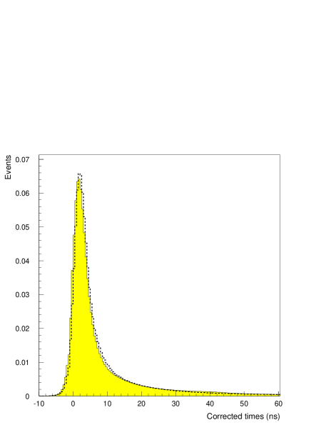
FIG. 19.: Corrected time distribution for Michel electrons from data (solid) and simulation (dashed) For $dist>35{\,{\rm cm}}$.

In Fig. 19 is a comparison of the hit time distribution for Michel events and the results of the simulation corrected for the event time and time-of-flight. These comparisons allowed fine-tuning of the parameter $A$, which in turn allowed estimation of the number of photoelectrons detected per unit $e^{\pm}$ energy.

A main ingredient of the photoelectron simulation was a model for the time distribution of emitted light. Cerenkov light was emitted promptly, but scintillation light was represented as having both fast and slow components [15]. Fluorescent reemmission was assigned the fast component only. A variety of resolution effects were taken into account either explicitly or implicitly via digitization and time calibration. The scintillation time parameters were then adjusted to match Michel electron data (see section 6.3.1) for PMT’s with single photoelectrons away from the $\check{\rm C}$erenkov cone. Apart from a small (arbitary) offset, agreement is good even though this does not necessarily mean that the underlying model is fully correct. Further comparisons to Michel data are addressed in sections 6.3 and 6.4.

6.   Event Reconstruction

6.1  Overview

The event reconstruction algorithm is discussed in section 6.2. In section 6.3 the extraction of the sample of electrons from muon decay in the tank is discussed together with the performance of the reconstruction algorithm on this sample. Section 6.4 is devoted to detector energy calibration using Michel electrons. Particle ID for neutrons and electrons is discussed in section 6.5. In section 6.6 the determination of the duty factor and its application to beam off subtraction is discussed.

6.2  Event Reconstruction Algorithms

The event reconstruction proceeded in four stages. The times of struck PMTs were adjusted by an algorithm which found the most appropriate time of a nearby cluster of tubes. Then an event vertex was reconstructed, followed by a search for a $\check{\rm C}$erenkov cone and finally verification that the distribution of times corrected to the vertex of the hit PMTs was appropriate.

The first step in the reconstruction process was to adjust the times of all PMTs with a pulse height that corresponded to fewer than 4 photoelectrons. The time of each of these PMTs was compared to the four nearest neighbors and the time of each channel was set to the earliest of these. This took account of the fact that signals with a small number of photoelectrons were distributed in time through the time spread of scintillation light and PMT dispersion so that the normal time slewing correction was ineffective. The use of this procedure improved the fit to the event appreciably. An initial estimate for the event time was made as the mean PMT time less 11 ns. The geometrical position of each struck PMT was then corrected to a position normal to its surface by a distance $v(t_{i}-t_{o})$, where $t_{i}$ was the PMT adjusted time, $t_{0}$ was the event time initial estimate, and $v=20{\,{\rm cm}}/ns$, the velocity of light in the liquid. The mean corrected position of the struck PMTs weighted by the square of the pulse height was used as an initial estimate of the event position.

A $\chi_{r}$ function was then formed as

$$\chi_{r}=\sum_{i}(t_{i}-t_{o}-r_{i}/v)^{2}\times W_{i}/(Q-6),$$

where i ran over all struck PMTs, $r_{i}$ was the distance from the PMT to the event vertex, $W_{i}$ was set to unity if $(t_{i}-t_{o}-r_{i}/v)$ was negative and to 0.04 if it were positive. $Q$ was the number of photoelectrons in the event. The quantity

$$(t_{i}-t_{o}-r_{i}/v)^{2}\times W_{i}$$

was limited to 1.5 ns². This weighting emphasized prompt $\check{\rm C}$erenkov light over scintillation light which tended to be delayed. An iteration was performed over $\pm x$, $\pm y$, $\pm z$ and $\pm t$ for the vertex first in steps of 25 ${\,{\rm cm}}$ (with an equivalent time using the velocity v above), and then 10 ${\,{\rm cm}}$ and finally 5 ${\,{\rm cm}}$ steps. If $\chi_{r}$ decreased at any iteration, then the vertex position was changed to the new value for the next iteration. The value of this $\chi$ was expected to offer discrimination between single short tracks and the more complicated pattern expected from neutrons.

An angle fit was performed for each event by constructing a

$$\chi_{a}=\frac{1+d/4}{2(Q-2)}\sum_{i}{(\theta_{i}-47.14^{o})^{2}\over 2\times(12^{o})^{2}}\times W_{i}\times\exp(r_{i}/14.9),$$

where $d$ was the distance of the event vertex from the center of the tank in meters, $Q$ was the number of photoelectrons in the event, and $\theta_{i}$ was the angle between the iterated direction and the vector from the fitted vertex and the tube i. $W_{i}$ was the PMT pulse height and $r_{i}$ was the distance from the vertex to the $i^{th}$ tube. An initial event time for this angle fit was set at 5 ns less than the starting time for position. A net of 26 angles was set up uniformly in $4\pi$. The minimum $\chi_{a}$ in this net determined an initial angle, a scan was then made in steps of 0.75 radians along the $\pm\theta$ and $\pm\phi$ directions to find a local minimum. The value of $\chi_{a}$ at this minimum was retained as a particle ID parameter. The ratio ${(\theta_{i}-47.14^{o})^{2}\over 2\times(12^{o})^{2}}$ was limited to 0.894 except in the “near” $\check{\rm C}$erenkov region $\cos\theta_{i}>0.927$ and $0.309>\cos\theta_{i}>0.052$, where it was set to 1.044.

The final discriminant in particle identification was the fraction of light emitted late in the event. Particles emitting $\check{\rm C}$erenkov radiation produced significant prompt light. A $\chi$ was constructed as the fraction of light after 12ns and was referred to as $\chi_{t}$.

Each of these $\chi$ parameters was sensitive to particle type through a measure of the complexity of the vertex, the existence of an identifiable $\check{\rm C}$erenkov ring and the time distribution of the light depending on $\check{\rm C}$erenkov light and the specific ionization of the particle in the event. A product was formed of the three $\chi$ as

$$\chi_{tot}=30\times\chi_{r}\times\chi_{a}\times\chi_{t}.$$

This parameter was effective in separating particle types. Quantitative tests of performance are discussed in section 6.3 on Michel electrons from muon decay and in section 6.5 on neutrons from cosmic rays.

6.3  Michel Electron Sample

6.3.1  Selection and Characteristics

Events that had veto activity in the $51.2{~{}\mu s}$ period previous to a primary event were dominated by decay electrons (Michel) from both positive and negative cosmic-ray muons that stopped in the detector. The time distribution of these events with respect to the veto signal is shown in Fig. 20.

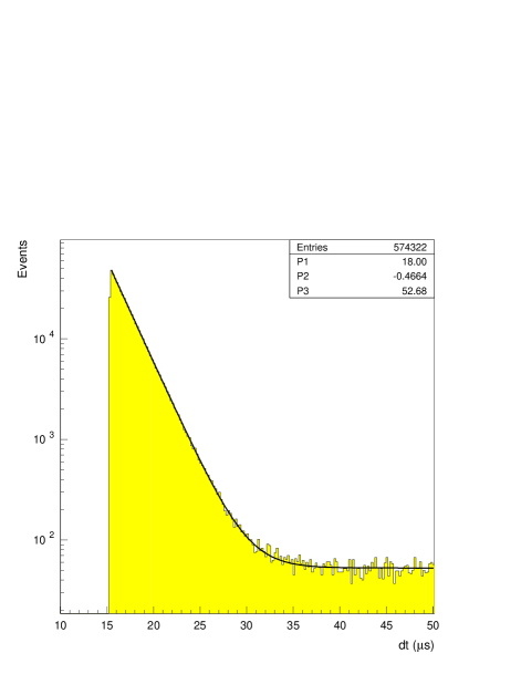
FIG. 20.: Distribution of times of tank events after veto activity. The constant P2 in the figure is the inverse of the lifetime of muons that remain after $15.2{~{}\mu s}$

Few events appear in the first $15.2{~{}\mu s}$ after the veto event because of an initial trigger condition which ignored events with veto activity in this time period, but there are still many events for analysis after this. Events were selected to be after $15.2{~{}\mu s}$ from the primary trigger in Fig. 20. The time distribution after $15.2{~{}\mu s}$ was fit with a functional form of a constant plus exponential with both amplitudes and the exponent variable. A satisfactory fit was obtained with a value of $2.15{~{}\mu s}$ for the exponent. This agreed with the expectation for a mixture of $\mu^{+}$ and $\mu^{-}$ (which has a $2.03{~{}\mu s}$ lifetime in mineral oil) for cosmic rays under the overburden existing in this experiment. The event sample from $15.2{~{}\mu s}$ to $30{~{}\mu s}$ after the primary has less than 1% accidentals as determined by the fit to the entire $50{~{}\mu s}$ range. This sample of $0.5\times 10^{6}$ events was used to map the gain of the detector as a function of position and angle throughout the volume, as is discussed in section 6.4 below. The response of the detector to particle ID was also mapped. The particle ID process is described in section 6.5. It should be noted that some accidental events in this sample were electrons from muons that decay but that had the decay muon misidentified.

6.3.2  Position Accuracy

The reconstruction process provided an event position via the $\chi_{r}$ minimization described in section 6.2. While there was no available direct measure of the accuracy of the position reconstruction, the distribution in the tank of reconstructed Michel electrons provided indirect evidence of reconstruction accuracy. Although it was not possible to determine the distribution of stopping muons in the detector to sufficient accuracy for this check, it was possible to verify that the distribution through the tank was smoothly varying and almost uniform. Additional evidence was available from $\nu_{e}C\to e^{-}X$ events, with a true distribution given by the $\approx 1/r^{2}$ falloff of DAR neutrino flux from A6. For both samples, Monte Carlo simulation of the electron provided the offset of the mean light-emission location from the point of origin of the electron.

A single variable, $dist$ was defined as the closest distance of an event to a surface passing through the photocathode surface of PMTs. Events behind this surface were assigned negative $dist$ values. In the LSND physics analyses, $dist$ was used to impose fiducial cuts. The cut values were chosen both to help suppress cosmic ray backgrounds, and to avoid the outermost region in which the tank response varied most rapidly (see section 6.4). Distributions of $dist$ on the known samples described above have shown that reconstructed electron positions tended to be systematically shifted away from the center of the tank (to lower $dist$) with respect to true positions. Quantifying this effect in the form of an acceptance correction for a given $dist$ cut required understanding the low-$dist$ regions well enough to estimate the consequences of selection cuts on these known samples. For a minimum $dist$ cut of 35 ${\,{\rm cm}}$, the resulting acceptance correction (ratio of the number of events reconstructed within the cut to the true number within the cut) ranged from 0.76 to 0.86. If this is due to a systematic shift, then for $dist$ near 35 ${\,{\rm cm}}$ the apparent shift of an event was about 15 ${\,{\rm cm}}$.

An estimate of reconstruction precision was obtained with neutrino events from $\nu_{\mu}C\to\mu^{+}X$. Both electrons and stopping muons were reconstructed for position, and the distance between the muon and the beginning of the electron track were compared. A distribution of this distance is shown in Fig. 21. This distribution agrees with the Monte Carlo simulation and gives an approximate vertex resolution of 20 ${\,{\rm cm}}$ for each particle.

FIG. 21.: Reconstructed distance between muon and decay electron for ${\nu_{\mu}}$ C scattering events. The smooth curve is a gaussian fit with parameters P1-P3 plus a constant (P4).

6.3.3  Angle Accuracy

The Michel electron sample was fit by the reconstruction algorithm described in section 6.2. In Fig. 22 is shown an angular distribution of charge weighted hit PMTs with respect to the fitted direction of the electron, together with results from the Monte Carlo simulation. These electrons have passed the same particle ID criteria as those that appear in Fig. 20.

FIG. 22.: Angular distribution of PMTs weighted by pulse height with respect to the fitted electron direction for muon decay electrons, data (solid) and Monte Carlo (dashed). The smooth curve is a fit to a constant (P4) plus gaussian with the parameters P1 - P3.

This distribution shows a clear peak due to $\check{\rm C}$erenkov light at cos $\theta\sim$ 0.68 and an approximately isotropic distribution due to reemitted $\check{\rm C}$erenkov light and scintillation light. The width of the peak is dominated by multiple scattering of electrons in the detector medium and agreed with the Monte Carlo simulation. The fine structure away from the $\check{\rm C}$erenkov peak is due to the weighting in position and angle fits. At 50 MeV, multiple scattering limited angular resolution to about $12^{\circ}$. In Fig. 23 is shown the angular distribution for neutrino induced electron events in the detector, where $\theta$ is the angle between the electron direction and the incident neutrino. The peak in the distribution at cos ${\theta}$ = 1 is from neutrino-electron scattering and had a width which confirms an angular spread of $\sim 12^{\circ}$ for electrons above 20 ${\,{\rm~{}MeV}}$.

FIG. 23.: Angular distribution for neutrino events with electrons in the final state with respect to the neutrino beam direction. The straight line is consistent in slope to that expected from $\nu_{e}$ C scattering.

6.4  Energy Calibration

Muons that stopped in the material of the detector were an excellent source for energy calibration. After a small background subtraction of non-correlated events, the charge distribution was fitted to a Michel decay spectrum convoluted with a Gaussian energy resolution function that gave the charge-to-energy conversion factor and the energy resolution at the endpoint. This Gaussian energy resolution was assumed to vary as $1/\sqrt{E}$, although results were not sensitive to the choice of energy dependence. A resolution of 7.7% at 52.8 ${\,{\rm~{}MeV}}$ was derived averaged over the entire volume with $dist>25{\,{\rm cm}}$. This sample was sufficiently large that it was possible to measure the endpoint energy for bins in a set of parameters discussed below. A fit was made to the Michel spectra to determine the energy response in each bin. Relative corrections were applied to set the end point of each of these spectra to 52.8 ${\,{\rm~{}MeV}}$. A correction was made for this variation by separating data into bins according to the value of parameters discussed below. These corrections were determined and applied sequentially. Overall run-number dependent correction factors were also applied. A fully corrected distribution is shown in Fig. 24. The fit to this distribution gave an energy resolution at the end point of 6.6%, a 15% improvement. In Fig. 25 is shown a comparison of the energy for a sample of Michel electrons together with a Monte Carlo calculation.

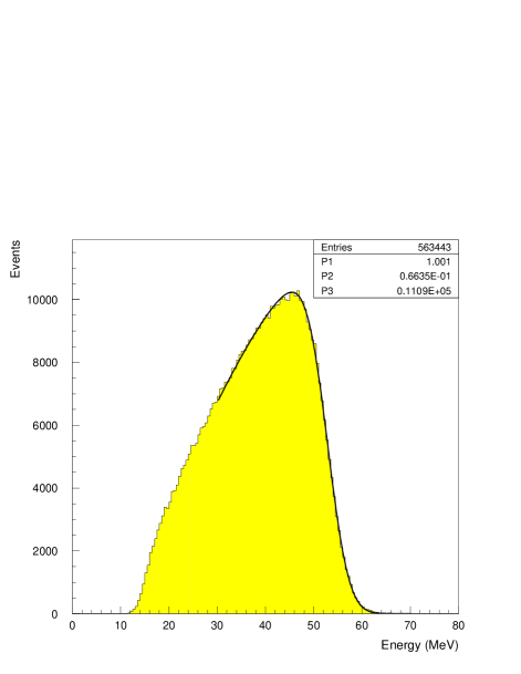
FIG. 24.: Electron energy distribution from stopped muon decay in the medium of the detector

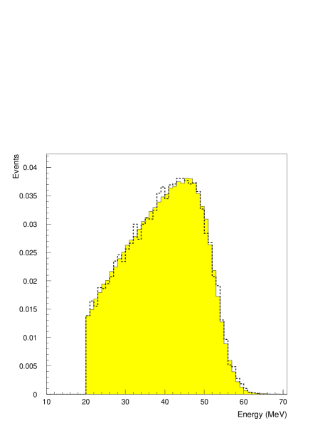
FIG. 25.: Charge distribution for Michel electrons from data (solid) and simulation (dashed)

Part of the calibration adjustment was due to physical processes understood from Monte Carlo simulation. In particular, the apparent charge deposited by an electron gradually increased as its position changed from the center of the tank to $dist\sim 25{\,{\rm cm}}$, and then dropped sharply in the outer regions of the tank. There were also variations depending on the direction of the electron with respect to the center of the tank. A comparison of charge distributions from Monte Carlo and data Michel events, as shown in Fig. 25 shows satisfactory agreement. The distributions agree well in shape, and a gain adjustment of $<10\%$ was consistent with expected uncertainties in the amount of scintillation light (the parameter $A$ in section 5.2) and overall gain factors. A second portion of the calibration adjustment was due to a periodic variation of the charge response of the QT cards with the relative phase of the event and the 100 ns clock. The remaining unexplained portion might be due to residual calibration inaccuracies; a mostly monotonic dependence on the reconstructed z position is in this category.

The energy response was corrected in bins in the following parameters: (1) The distance from the PMT face to the reconstructed position of the electron ($\pm 3\%$); (2) The relative phase between PMT hits and the 100 ns clock ($\pm 3.5\%$); (3) The cosine of the angle between the reconstructed electron direction and the position vector from the center of the tank. ($\pm 7\%$); (4) Reconstructed position along the z axis of the detector($8\%,4\%$); (5) The angle of the reconstructed direction with respect to the y axis. ($\pm 1.5\%$). The numbers in parentheses are full ranges of typical variation for 1994 and 1995 data respectively. Because some of the effects were correlated, these ranges may not represent the full underlying variations. Corrections were made iteratively until the remanent corrections were less than $\pm 0.5\%$. The resolution was found to be $\approx 1\%$ larger in the outermost part of the fiducial volume than in the center of the tank. In a forthcoming publication [30] an analysis of ${\nu_{e}}$ on ${}^{12}C$ scattering to an electron and the ground state of nitrogen, ${}^{12}N_{gs}$ will be described. For this reaction the end point of the electron spectrum is at 35.4${\,{\rm~{}MeV}}$ and the endpoint of the $\beta$ decay spectrum from ${}^{12}N_{gs}$ is at 16${\,{\rm~{}MeV}}$. Each of these end points verified the expected linearity of the detector for electron energy in this range.

6.5  Particle Identification

During normal operation, primary events had fewer than four hit PMTs in the veto in time. To obtain a sample of cosmic ray neutrons, these events were subsequently required to have a correlated 2.2-MeV ${\gamma}$ using criteria described in reference [6] and to occur in the beam-off part of data taking. From the distribution of time between the primary signal and the correlated ${\gamma}$ signal it was determined that the selected sample consisted of 90% neutrons. This set of events was used as a “neutron” sample to verify the operation of the particle identification algorithm. The “neutron” sample was then limited in deposited energy in the detector to correspond to that for electrons of kinetic energy between 36 and 60 ${\,{\rm~{}MeV}}$. A sample of electron candidates was selected from the “Michel” data set as described above. The particle identification algorithm using spatial reconstruction, angular reconstruction, and late light criteria was applied, and a histogram of the particle ID parameter is shown in Fig. 26 for electrons and for identified neutrons.

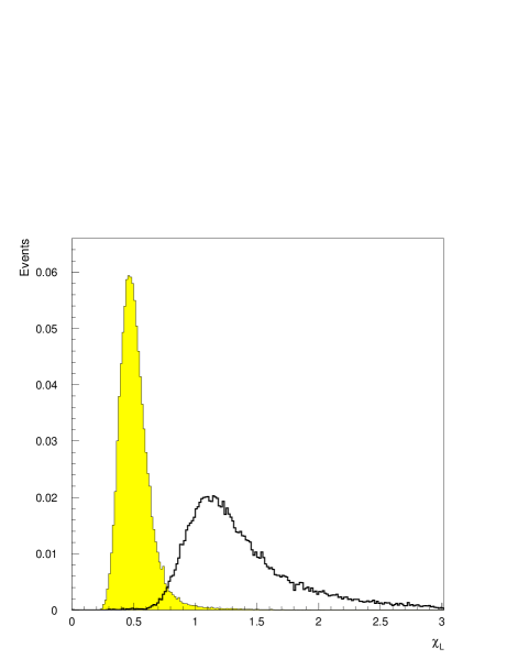
FIG. 26.: Particle ID parameter for “ electrons” (shaded) and “neutrons”.

These distributions show the difference between electrons and neutrons as identified by a correlated ${\gamma}$. Events were selected based on individual $\chi$ parameters and then finally a cut on the particle ID parameter at $\chi_{tot}$ = 0.65 gave 95% efficiency for selecting electrons above $36{\,{\rm~{}MeV}}$, and a rejection of 10^-3 against neutrons. Details of this analysis may be found in [6].

6.6  Duty factor measurements

The fraction of the time that the beam was on is referred to as the duty factor. The duty factor was subject to variation during the course of data taking from two basic sources. The accelerator operated in approximate synchronism with the AC line frequency. The AC line frequency varied in the course of a 24 hour period so that the time of AC zero crossing could be different by as much as a few seconds from uniform time, implying that the accelerator start time varied also. Under normal operation, the duration of the beam pulse was constant and controlled by a precise clock in the accelerator complex. The effect of this AC variation was to induce a small variation in the duty factor. In practical terms however, this variation was negligible. Accelerator operation was very sensitive to beam loss, and whenever significant loss was detected, the ion source current was interrupted and acceleration was terminated. This caused significant variation in the length of the beam pulse and, hence, a short term variation in the duty factor. Under tuning of the accelerator for minimum beam loss, this condition occasionally persisted for periods that caused the duty factor to vary significantly. An H⁺ signal was asserted during beam acceleration and for a short period both ahead and after the actual accelerating period, as described in section 2.1.2. The variation of the duty factor from beam duration variations was the largest effect and amounted to as much as 10% over periods of minutes. The duty factor was determined from the ratio of the number of primary triggers that occur when the H⁺ signal was on to all primary triggers and was found to be $0.065\pm 0.001$ in 1993 - 1995. Genuine neutrino interactions represented only $\sim 10^{-5}$ of all triggers and were a negligible perturbation of the ratio. Beam induced events that were not neutrino induced were much less than neutrino induced events and were also negligible. A ratio of these counts was made over the entire data taking period. This ratio was then used to multiply the event rates that occurred during beam-off time to estimate a corresponding rate for beam-on and, hence, provide a sample for background subtraction. Although the exact duty factor should be calculated as a function of time and an average taken, it was determined that the ratio of counts for H⁺ on to off, each separately averaged over the data taking period, was the same for first order variations of the instantaneous duty factor and of the gain of the detector.

The duty factor was also determined for ${\gamma}$ events (PMT hits $<100$), $\beta$ events ($100<$PMT hits $<250$), and higher energy events (PMT hits $>250$) and found to be the same within errors. Knowing the duty factor, a beam-on minus beam-off subtraction was performed to remove the background from beam-unrelated processes. For a duty factor of $0.065\pm 0.001$, the ratio of beam-on events to beam-off events was $0.070\pm 0.001$. Therefore, for any event sample the net number of beam-related events is the number of beam-on events minus 0.070 times the number of beam-off events.

7.   Conclusion

In conclusion, the construction of the LAMPF neutrino source has been described, including calculations of neutrino flux from the each of the relevant reactions from pions and muons for each of the three years of operation. The expectation that this source will have a low contamination from $\bar{\nu}_{e}$ has been justified. The construction and operation of the detector has been discussed with a description of salient operating parameters. The detector has performed well and has been well suited for the measurement of low energy neutrino interactions with both electrons and muons as the final state lepton. Future publications will discuss the search for neutrino oscillations and the measurement of neutrino-carbon scattering.

Acknowledgements

This detector system has relied on the efforts and support of many people in addition to the authors. Camilo Espinoza, Greg Hart and Neil Thompson have been crucial to the construction and maintenance of the system. Butch Daniels, Bill Marterer, and Suzy Weaver were also central to the construction effort. Mike Sullivan contributed in the early stages of the experiment. Conventional construction was important to this experiment and Bill Wassmund as construction manager proved invaluable. Earl Hoffman and the accelerator operations personnel produced beam of excellent quality throughout the data taking period. The beam stop and neutrino source were demanding to operate at the radiation levels that were routinely encountered, and the efforts of Dick Werbeck and his group are truly appreciated. We were extremely fortunate to have had many undergraduate students who made substantial contributions to the experiment; they were acknowledged by name in a previous letter. This experiment was built and carried out in a difficult period for this facility; without the support of Peter Barnes, Cyrus Hoffmann and John McClelland this work would not have been completed. This work was directly supported by the U. S. Department of Energy and by the National Science Foundation.

REFERENCES

- [1] A proposal to Search for Neutrino Oscillations with High Sensitivity in the Appearance Channels and , LA-11842-P.
- [2] C. Athanassopoulos, et. al. , Phys. Rev. Lett. 68, 274 (1995).
- [3] To be submitted to Phys. Rev. C.
- [4] R. L. Burman, M. E. Potter, and E. S. Smith, Nucl. Instrum. Methods A291, 621 (1990).
- [5] C. H. Llewellyn Smith, Physics Reports 3, 262 (1972); E. J. Beise and R. D. McKeown, Comm. Nucl. Part. Phys. 20, 105 (1991).
- [6] To be submitted to Phys. Rev. C.
- [7] J. A. McGill, et. al. , Los Alamos National Laboratory Report LA-8937T (1981); J. L. Langenbrunner et. al. , Nucl. Instrum. Methods A 325, 187 (1993).
- [8] R. C. Allen, et. al. , Nucl. Instrum. Methods A 284, 347 (1989).
- [9] R. C. Allen, et. al. , Phys. Rev. D 47, 11 (1993).
- [10] R. L. Burman, et. al. Nucl. Instrum. Methods A 368, 416 (1996), Forschungszentrum Karlsruhe Report FZKA 5595 (1995);
- [11] F. Herzog and K. Alder, Helv. Phys. Acta. 53 (1980) 53.
- [12] T. Suzuki, D. F. Measday, J. P. Roalsvig, Phys. Rev. C 35, 2212 (1987).
- [13] Hamamatsu Photonics K. K. Photomultiplier type no. R1408.
- [14] J. J. Napolitano, et. al. , Nucl. Instrum. Methods A 274, 152 (1989).
- [15] R. A. Reeder et. al. , Nucl. Instrum. Methods A 334, 353 (1993).
- [16] The oil was obtained from IGI Petroleum Specialties, Inc. NJ.
- [17] Nitrogen dye laser from Laser Photonics Inc type LN203c.
- [18] Ludox was made by Dupont Chemicals, East Chicago, Indiana. It was a colloidal suspension of 22nm quartz spheres with a mean free path of about 1.6 cm.
- [19] Global Positioning System, Kinemetrics True Time, Santa Rosa CA95407 Model GPS DC Mk III.
- [20] Motorola type MC10319.
- [21] Motorola MVME 167/D1 Single Board Computer, Motorola Inc. Tempe AZ 85282 (1991).
- [22] Silicon Graphics Inc SGI 4D/480 multiprocessor computor.
- [23] CEBAF On-line Data Acquisition. This code was developed at CEBAF and an early version was tested and debugged in this installation by this collaboration.
- [24] I. Stancu, Computing in High Energy Physics ’94 (Proceedings of the Conference on Computing in High Energy Physics April 1994), LBL Report 35822, 343 (1995).
- [25] K. McIlhany, D. Whitehouse, A. M. Eisner, Y-X. Wang and D. Smith, Computing in High Energy Physics ’94 (Proceedings of the Conference on Computing in High Energy Physics April 1994), LBL Report 35822, 357 (1995).
- [26] J. B. Birks, Pergamon Press, Oxford 1964.
- [27] Review of Particle Properties, Phys. Rev. D 50, 1173 (1994).
- [28] R. L. Craun and D. L. Smith, Nucl. Instrum. Methods 80, 239 (1970).
- [29] M.E. Moorhead and N.W. Tanner, Oxford Report OUNP-91-05 (1991).
- [30] To be submitted to Phys. Rev. C.