Measurement of Propagation Time Dispersion in a Scintillator

Abstract

One contribution to the time resolution of a scintillation detector is the signal time spread due to path length variations of the detected photons from a point source. In an experimental study a rectangular scintillator was excited by means of a fast pulsed ultraviolet laser at different positions along its longitudinal axis. Timing measurements with a photomultiplier tube in a detection plane displaced from the scintillator end face showed a correlation between signal time and tube position indicating only a small distortion of photon angles during transmission. The data is in good agreement with a Monte Carlo simulation used to compute the average photon angle with respect to the detection plane and the average propagation time. Limitations on timing performance that arise from propagation time dispersion are expected for long and thin scintillators used in future particle identification systems.

, , , , , , , , , , , , , , and

1 Introduction

There has been recent interest in the timing performance of long and thin plastic scintillation detectors with demands on the time resolution of 100 ps and below, e.g. for the future $\overline{\mbox{P}}$ANDA experiment at FAIR PANDA . An existing experiment with a challanging scintillator system is COMPASS with the installation of the 2.8 m long and 4 mm thin recoil detector under way COMPASS . This paper shows that the detector performance required by these experiments is close to the fundamental limit that arises from the statistical fluctuations in the process of the signal generation.

At $\overline{\mbox{P}}$ANDA , the identification of charged particles with momenta up to several GeV$/c$ will be performed by the detection of internally reflected Cherenkov (DIRC) light DIRC-GSISciRep05 . Any measurement of the time-of-propagation (TOP) in the DIRC counter needs a precise time reference and can be combined with the time-of-flight (TOF) information from long scintillator slabs in front of the radiator barrel of the DIRC. Within the almost fully hermetic $\overline{\mbox{P}}$ANDA detector such a scintillator array needs to be as thin as physically possible. At COMPASS, it is the need for a low momentum proton detection that requires the scintillators to be very thin.

The timing properties of scintillators are usually defined in terms of a coincidence time resolution. In a typical laboratory measurement the time difference between the discriminated signals of two photomultipliers (PMTs) placed at the extremes of a sample of scintillator is measured for minimum ionising particles crossing the scintillator at its centre. For small counters of 45 cm length and 20 mm thickness a time resolution reduced for one PMT of the order of FWHM $\approx$ 150 ps has been achieved by the authors in the laboratory. For long scintillators there are several effects degrading the time resolution, namely the light attenuation and the consequences of the scintillator acting as a light guide with corresponding propagation time dispersion.

First photoelectron timing errors have been evaluated for slow scintillators (BGO, $\tau_{\mathrm{decay}}\approx 300$ ns) and larger amplitudes (number of photoelectrons $N>30$) previously Petrick1991 ; Clinthorne1990 , but not for fast plastic scintillators and small amplitudes, where the achievable timing performance depends also on path length variations. The purpose of this paper is to discuss expressions for the timing error which include propagation time dispersion and to verify experimentally the the correlation between signal time and average photon angle at the read-out end of a scintillator.

2 The Origin of Time Jitter in Scintillator Timing

One fundamental limit on the time resolution of scintillation counters comes as a consequence of the statistical processes involved in the generation of the signal. Post and Schiff PostSchiff1950 have first discussed such limitations. In general, the voltage pulse of a photomultiplier, $V_{\mathrm{PMT}}$, can be expressed as a linear superposition of $N$ single photoelectron pulses, $v_{i}$, whose amplitude is allowed to vary due to gain fluctuations, $g_{i}$, governed by a measurable probability distribution. The pulses arrive at individual times due to the time spread in the energy transfer to the optical scintillator levels, $t_{\mathrm{dep}}$, the decay time of the light emitting states, $t_{\mathrm{emit}}$, the propagation time, $t_{\mathrm{prop}}$, and the transit time, $t_{\mathrm{TT}}$, being the time difference between photo-emission at the cathode and the arrival of the subsequent electric signal at the anode. In addition, there is white Gaussian electronic noise, $w(t)$. We incorporate these processes into a general model: $V_{\mathrm{PMT}}(t)=\sum_{i=1}^{N}{g_{i}v_{i}(t-(t_{\mathrm{dep}}+t_{\mathrm{emit}}+t_{\mathrm{prop}}+t_{\mathrm{TT}})_{i})}+w(t)$, where $N$ fluctuates from one pulse to another. In a semi-classical model the probability for observing $N$ photoelectrons during a time interval $T$ is given by a Poissonian distribution $P(\overline{N},N)$ with $\overline{N}$ being the mean number of photoelectrons per pulse.

The following calculation is focused on the limitations arising from the contribution of the path length variation. Central to the calculation is the relation between initial axial angle, $\theta$, and propagation time: $t=Ln/(c\cos\theta)$, for a point like source of light placed at a distance $L$ from the end face of a cylindrical scintillator with refractive index $n$ in a medium of refractive index $n_{\mathrm{ext}}$, where $\theta_{\mathrm{max}}$ represents the complement of the total internal reflection angle, $\theta_{\mathrm{max}}=\arccos{n_{\mathrm{ext}}/n}$. In the case of a rectangular shaped scintillator the relation is still valid as can be seen from the following consideration: in any reflection the change in the velocity vector of a particular photon takes place in the direction perpendicular to the face it hits. The component of this vector along the longitudinal axis remains unchanged during the whole motion and therefore the propagation time only depends on the initial axial angle, distance to the PMT, and index of refraction. Consequently, a detector displaced by a distance $d$ from the end face of the scintillator would link in one linear dimension the angle and propagation time with an accuracy given by $\sigma_{\theta}\approx\sqrt{t_{x}^{2}/12+a_{x}}/d$, where $t_{x}$ is the thickness of the scintillator and $a_{x}$ the aperture of the detector.

For a quantitative description including extended light sources, light attenuation and refraction a full photon tracking simulation with the correct geometry of the set-up and a good model of scintillation light excitation and emission was needed. A general purpose Monte Carlo program Gentit2002 simulating light propagation was used to compute the average photon angle with respect to the detection plane and the average propagation time.

Experimentally, the quality of a scintillator surface limits the conservation of photon angles. Small geometrical inhomogeneities can have a strong impact on the transmission of photons and then the correlation between detection position and propagation time is heavily affected. There is no straight forward method for the estimation of the parameters necessary for an appropriate simulation of the surface quality. In fact, a Monte Carlo refractive index matching technique was developed only very recently to determine these parameters Wahl2007 . It was therefore mandatory to perform an experiment with a sample of plastic scintillator in order to investigate empirically the mentioned correlation.

In an experiment the discriminators and any noise in the electronic circuits contribute to the time spread. Further, the response time of discriminators may shift with signal amplitude (”time walk”). Time walk effects are relevant if a large range of amplitudes is discriminated and can get corrected by various means, either in hardware or software.

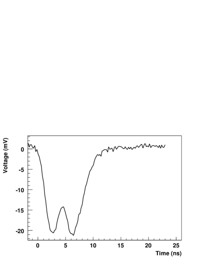
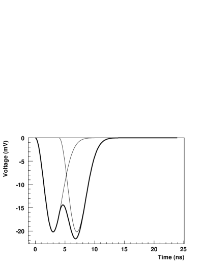
Figure 1: Left: Typical PMT voltage pulse for low light intensities as measured with a digital oscilloscope. Right: Typical voltage pulse calculated by a Monte Carlo method for two single photoelectron pulses separated by 5 ns.

It is a standard in nuclear physics to use constant fraction discriminators (CFD) and leading edge discriminators (LED), the latter showing a characteristic time walk. In many cases constant fraction timing provides the best time resolution with scintillation counters. The situation is significantly different when the number of photons is small. In this case the sampling of the arrival time distribution is poor and the signal shape is very variable. Fig. 1 shows the trace of a PMT voltage pulse for low light intensities as measured with a digital oscilloscope and the result of a Monte Carlo calculation for $N=$ 2 photoelectrons. The voltage pulse of a single photoelectron was modelled by $v_{\mathrm{spe}}(t)=gct^{2}\e^{-{t^{2}}/{\tau^{2}}}\!/\int_{0}^{\infty}t^{2}\e^{-{t^{2}}/{\tau^{2}}}\!\mathrm{d}t$, where $g$ is the gain of the PMT, $c$ is the conversion factor for charge to voltage and $\tau$ has been chosen to be 4 ns in order to match the signal of the PMT used in the experimental set-up. A large distribution of pulse shapes reflecting the different arrival times of the individual photons is possible and the confounding effect of the overlapping single photon responses leads to problems with leading edge and peak detectors. Thus, the timing performance in the pile-up case degrades considerable from single photon timing.

3 Calculation of Fundamental Limits from Propagation Time Dispersion

The spread of propagation times is given by $\Delta t_{\mathrm{prop}}=Ln/c(\cos^{-1}{\theta_{\mathrm{max}}}-1)$ for the minimum and maximum propagation times of meridional rays, $t_{\mathrm{min}}=Ln/c$ and $t_{\mathrm{max}}=Ln/(c\cos\theta_{\mathrm{max}})$. The probability density function of the propagation times of photons, $\mathrm{d}N/(N\mathrm{d}t)$, produced by an event at $t=0$, can be calculated from the angular distribution of photons inside the scintillator, $\mathrm{d}N=2\pi\,\mathrm{d}\cos\theta$. It follows that $\mathrm{d}N/\mathrm{d}t=-2\pi\,Ln/(ct^{2})$ and $N=\int_{t_{\mathrm{min}}}^{t_{\mathrm{max}}}(\mathrm{d}N/\mathrm{d}t)\mathrm{d}t^{\prime}=2\pi\,(\cos\theta-1)$. Finally, the probability density for the arrival times at the photocathode due to path length variations is $P_{\mathrm{prop}}(t)=\mathrm{d}N/(N\mathrm{d}t)=Ln/((\cos\theta-1)ct^{2})$.

The arrival time probability density function for a realistic scintillator can be folded in as follows: $P(t)=\int_{0}^{\infty}I(t^{\prime})P_{\mathrm{prop}}(t-t^{\prime})P_{\Lambda}(t-t^{\prime})\mathrm{d}t^{\prime}$, where $P_{\Lambda}(t)=\exp{-tc/(n\Lambda)}$ is survival probability depending on the bulk absorption coefficient, $\Lambda$, in the material. The distribution of decay times of light emitting states is included with a light pulse shape of the form: $I(t)=[(e^{-t/\tau_{2}}-e^{-t/\tau_{1}})/(\tau_{2}-\tau_{1})+Re^{-t/\tau_{3}}/\tau_{3}]/(1+R)$, where $\tau_{1}$ and $\tau_{2}$ are two fast decay constants, $\tau_{3}$ corresponds to the decay time of the slow component, and $R$ is the ratio of the slow to fast components. For the parameters of emission time distribution values of $\tau_{1}=$ 0.9 ns, $\tau_{2}=$ 2.1 ns, $\tau_{3}=$ 14.2 ns, and $R=$ 0.27 were chosen. Comparable values are given in Ref. Nam2002 . The probability density function of the transit time spread of electrons in the photomultiplier, $P_{\mathrm{TTS}}$ is not relevant for the following discussion, since micro-channel plate PMTs provide an alternative with excellent timing capabilities. Analytical descriptions of the probability density functions describing the time jitter of photoelectrons generated at the photocathode have been discussed before, e.g. in Moszynski1979 .

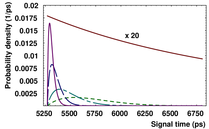
Figure 2: Calculated distributions of signal times for $L=$ 1 m, $n=$ 1.58, for an increasing number of photoelectrons, $N$, at a fixed threshold of $N_{\mathrm{thr}}=$ 2: $N=$ 5 (solid line), $N=$ 10 (dashed line), $N=$ 25 (dot-dashed line), and $N=$ 50 (dotted line). The continuously falling (solid) line is a calculation for single photoelectron pulses ($\times$ 20).

The probability for a photoelectron to be detected in the interval between $t_{\mathrm{min}}$ and $t$ is $p(t)=\int_{t_{\mathrm{min}}}^{t}\!\mathrm{d}N/(N\mathrm{d}t)\mathrm{d}t^{\prime}$. Assuming a Poissonian distribution for the probability that a definite number of photoelectrons, $N_{\mathrm{thr}}$, has been accumulated leads to the signal time distribution $S(t)=N\frac{\mathrm{d}N}{\mathrm{d}t}{N-1\choose N_{\mathrm{thr}}-1}[p(t)]^{N_{\mathrm{thr}}-1}[1-p(t)]^{N-N_{\mathrm{thr}}}$, which is to be normalised for getting the probability density function. Calculated distributions for signal times with $L=$ 1 m, $n=$ 1.58, for an increasing number of photoelectrons in the pulse, $N=$ {5, 10, 25, 50} and $N_{\mathrm{thr}}=$ 2, as well as for single photoelectron pulses ($\times$ 20) are shown in Fig. 2.

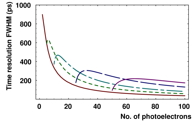
Figure 3: Calculated limits on time resolution (FWHM) for $L=$ 1 m, $n=$ 1.58, as a function of the number of photoelectrons, $N$, at thresholds of $N_{\mathrm{thr}}=$ 2 (solid line following a FWHM $\propto 1/N$ dependence), $N_{\mathrm{thr}}=$ 5 (dotted line), $N_{\mathrm{thr}}=$ 10 (dot-dashed line), $N_{\mathrm{thr}}=$ 25 (dashed line), and $N_{\mathrm{thr}}=$ 50 (solid line).

The limit on time resolution arising from statistics of photon detection can now be calculated using the relations for the expectation values $\langle t_{p}\rangle=\int_{t_{\mathrm{min}}}^{t_{\mathrm{max}}}\!tS\mathrm{d}t$ and $\langle t_{p}^{2}\rangle=\int_{t_{\mathrm{min}}}^{t_{\mathrm{max}}}\!t^{2}S\mathrm{d}t$, and the variance of the signal time $\mathrm{Var}(t_{p})=\langle t_{p}^{2}\rangle-\langle t_{p}\rangle^{2}$. The time resolution (FWHM) for $L$= 1 m, $n$= 1.58 as a function of $N$ is shown in Fig. 3 for a range of thresholds, $N_{\mathrm{thr}}$= {2,5,10,25,50}. The curve for $N_{\mathrm{thr}}$= 2 follows a FWHM $\propto 1/N$ dependence.

4 Experimental Set-up

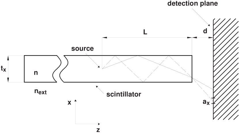
Figure 4: Schematic representation of the arrangement of scintillator and detection plane at a distance $d$. The paths of two photons leaving the scintillator at the same point are shown. Typical parameters for the experiments were $a_{x}=a_{y}=$ 3 mm, $L=100$ cm, $d=10\,$mm, $t_{x}=32$ mm, and $t_{y}=10$ mm.

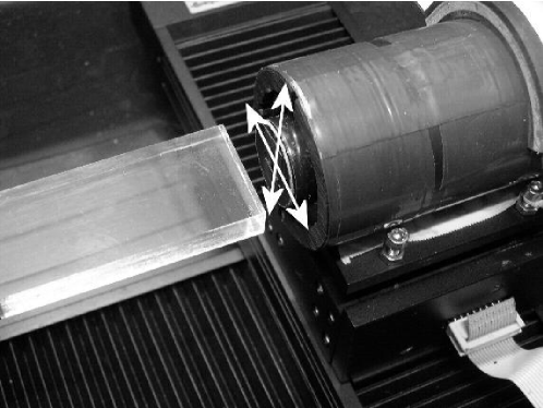
Figure 5: The photograph shows the crossed positioning units and the PMT equipped with a plastic mask with a square aperture of 3 mm $\times$ 3 mm. The PMT motion takes place in the plane perpendicular to the longitudinal axis of the scintillator.

The basic idea was to measure the average photon angle with respect to the detection plane at a distance $d=$ 1 cm. A schematic representation of the arrangement of scintillator and detection plane is given in Fig. 4. The trajectories of two photons leaving the scintillator in the same point are shown. A BC-408 scintillator from Bicron of dimensions $32\times 10\times 2000$ mm³ was used. The scintillator is characterised by a decay time of $\tau_{\mathrm{decay}}=$ 2.1 ns, a small admixture of a slower decay time, and a refraction index of $n=$ 1.58. It was important for the conservation of photon angles that the faces of the scintillator were not wrapped or covered. A minimum contact area of the bar at only two edges was accomplished by placing the scintillator along the longitudinal axis of a black metallic tube of the proper dimensions. The two tubes of 1 inch diameter were of type R4998 from Hamamatsu with a fast time response and a linear focused dynode structure of 10 stages, leading to a transit time spread of only $\sigma_{\mathrm{TTS}}=$ 160 ps. At one end the reference PMT was fixed keeping contact with the scintillator by a suitable set of springs. At the other end a set of two linear positioning stages permitted the scanning of the detection plane behind the scintillator, see Fig. 5. A thin plate with a 3 mm wide aperture was mounted in front of the PMT window to limit the acceptance. A ⁹⁰Sr source and a fast pulsed ultraviolet laser from Horiba Jobin Yvon were used for the measurements. The laser had a pulse duration FWHM $<200$ ps. The signals were digitised by a charge integrating analogue-to-digital converter (LeCroy 1885F, 50 fC$/$count) and by a LeCroy time-to-digital converter (LeCroy 1875, 25 ps$/$count). The TDC digitisation corresponds to an accuracy of 25$/\sqrt{12}$ ps $\approx$7 ps.

A full scanning of the amplitudes was performed by means of filters placed in front of the movable PMT. The constant fraction discriminators showed little time walk ($\Delta t/\Delta Q<0.7$ ps$/$pC). It was fitted and used for the correction of the TDC information.

5 Discussion of Results

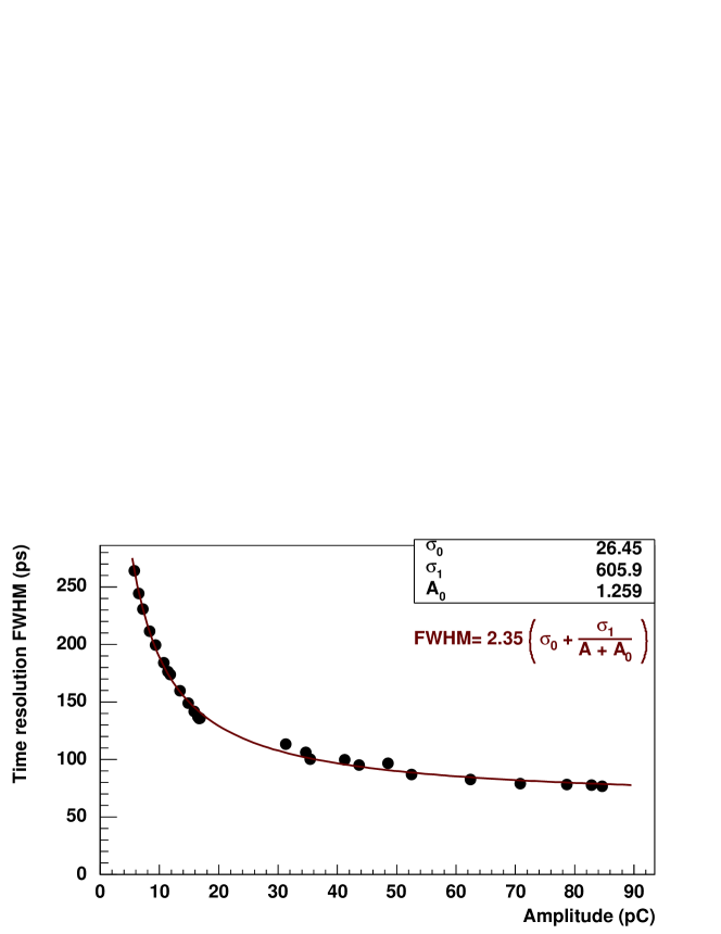
Figure 6: Measured time resolution (FWHM) obtained with a BC-408 scintillator and an UV laser of varying primary light intensity as a function of the amplitude, $A$. The function FWHM $\propto\sigma_{0}+\sigma_{1}/(A+A_{0})$ has been fitted to the data.

A time resolution of FWHM $\approx 130-260$ ps was achieved for low amplitudes, see Fig. 6. With increasing amplitude the resolution improved until it levelled off at about FWHM $\approx 80$ ps, demonstrating that at high intensities the photon statistics is no longer decisive and the resolution is supposedly dominated by electronic noise. A function of the form FWHM $\propto\sigma_{0}+\sigma_{1}/(A+A_{0})$ has been fitted to the data under the assumption that the detector response becomes Gaussian as the number of photoelectrons increases.

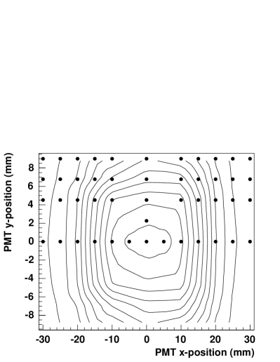
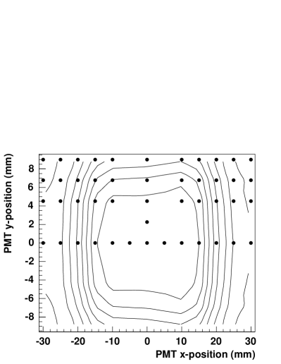
Figure 7: Measured signal time (right) and amplitude (left) as contour lines for the two dimensional scanning performed at a distance of 1 cm from the end face of the scintillator. The PMT positions for the data points are superimposed. The steps between contour lines correspond to 100 ps and $-$100 ADC channels, respectively.

Fig. 7 shows the positions of the aperture in the detection plane as points in the x- and y-dimension. For each point signal time and amplitude have been measured at a distance of 1 cm from the end face of the scintillator. Only the upper half plane was scanned due to the symmetric behaviour of all observables expected on grounds of the geometrical symmetry. The points are superimposed on the measured data presented as contour lines with steps of 100 ps in signal time (right) and steps of $-$100 channels in amplitude (left). The signal time variation takes place earlier in the y-direction. The width of the scintillator in this direction is 10 mm to be compared to 32 mm for the perpendicular one.

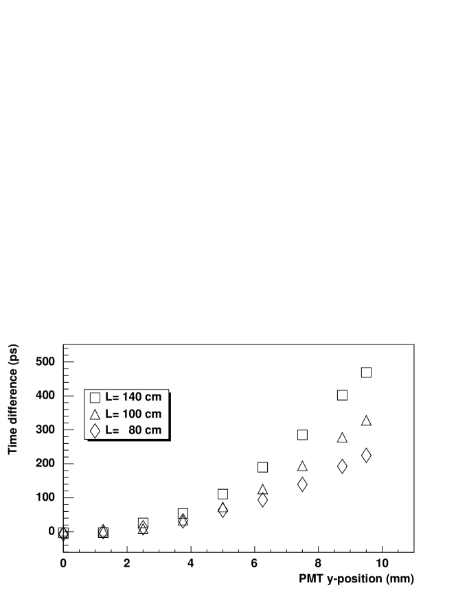
Figure 8: Measured signal time as a function of the aperture position when the scintillator is excited by the UV laser at three different positions, $L=$ 80, 100, and 140 cm.

To exclude any amplitude dependent time shifts this experiment was repeated for three different positions of the laser source, adjusting the laser light intensity to equal PMT output signals for the central aperture position. Fig. 8 shows the variation of the signal time as a function of the position of the aperture with respect to the centre, when the laser light is injected at $L=$ 80, 100, and 140 cm. A signal time difference approximately linear with the distance for a given aperture position was observed.

In a perfect scintillator the portion of the light cone that lies inside the total internal reflection angle is transported undistorted to the end of the slab. Since the transmission involves many reflections, the exit angle from a real scintillator is dependent on the sharpness of its edges and the parallelism of its faces. The measurements showed an unambiguous correlation between signal time and tube position and demonstrated an sufficient conservation of axial angles. The observed correlation is not masked by a change of apparent anode sensitivity with angle of incidence at the photocathode. Although, the photomultiplier tube sensitivity depends on the incident angle since the path length of a photon through the photocathode increases like $1/\cos\theta$ giving a corresponding higher probability for the emission of a photoelectron Hamamatsu1999 . The subsequent course of this electron is, however, not simple and the cosine law can only be considered as a first approximation. It would imply that at non-central aperture positions amplitude losses get partly compensated and effects of the propagation time dispersion get emphasised. The angular variation of quantum efficiency and the reflectance of a PMT entrance window were measured recently Shibamura2006 , showing a larger photon-to-photoelectron conversion efficiency for incident angles $\theta>45^{\circ}$ than that at $\theta>0^{\circ}$, however, the reflectance is also significantly larger at these angles.

Fig. 9 shows measured signal time (top) and amplitude (bottom) as a function of horizontal and vertical aperture position for the PMT at central position. Empty circles represent mirrored points. An analysis of the data reveals that the observed change in signal time is not following the change in signal amplitude. The light propagation is simulated in detail with the Monte Carlo code where first photoelectron timing was implemented. The observed variation of signal time and amplitude with position was verified, as shown in Fig. 10. The code was then used to simulate the average photon angle with respect to the detection plane as a function of the horizontal and vertical aperture position, see Fig. 11. The good agreement between data and Monte Carlo together with the simulated relation between aperture position and angle verified that the propagation time dispersion has been observed. The measured time differences are in fair agreement with the spread of propagation times when applying the simple $t_{A}-t_{B}=Ln/c(\cos^{-1}{\theta_{A}}-\cos^{-1}{\theta_{B}})$ formula to a pair of simulated incident angles $\theta_{A/B}$ at two aperture positions $x_{A/B}$ or $y_{A/B}$.

The code was also used to simulate the time resolution of a full coverage PMT as a function of the number of photoelectrons. These simulations served as a guide for detector developments Achenbach-GSISciRep05 . One example, where the contribution of the propagation time spread $\sigma_{\mathrm{prop}}$ gets significant is given by the cylindrical TOF counter being developed for $\overline{\mbox{P}}$ANDA PANDA . A thickness of only 5 mm would allow to mount the scintillator strips together with the DIRC radiators, but reduces the number of photoelectrons to $\langle N_{\mathrm{pe}}\rangle\simeq 100$ for particles crossing a scintillator at $L=1$ m. The Monte Carlo simulation including the finite decay time of the scintillator predicts a minimum achievable time resolution of FWHM${}_{\mathrm{min}}\simeq 150$ ps, depending a little on threshold.

These results have brought forward the idea of improving the time resolution of a scintillation counter through position sensitive photon detection. An analogy of this method is used successfully in DIRC-like detectors using glass slabs for measuring the Cherenkov angle, but was never investigated in scintillators.

Lower bounds on scintillation detector timing performance have been developed in the past for moderate or relatively high total light output, addressing the exponential decay of the light intensity and non-ideal photodetectors Clinthorne1990A . These bounds can be useful in determining performance sensitivity to scintillator and PMT parameters. To the authors’ knowledge the path length variation in long scintillators as a source of additional time dispersion has not been included in the models.

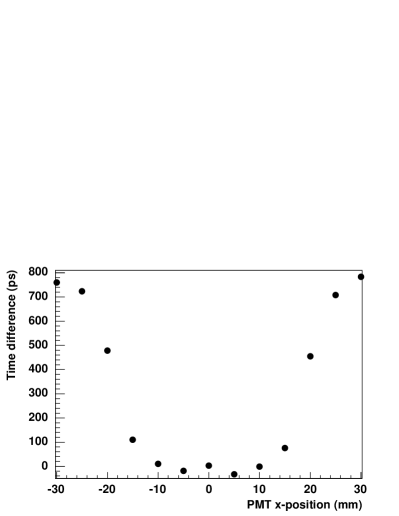
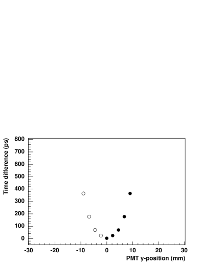
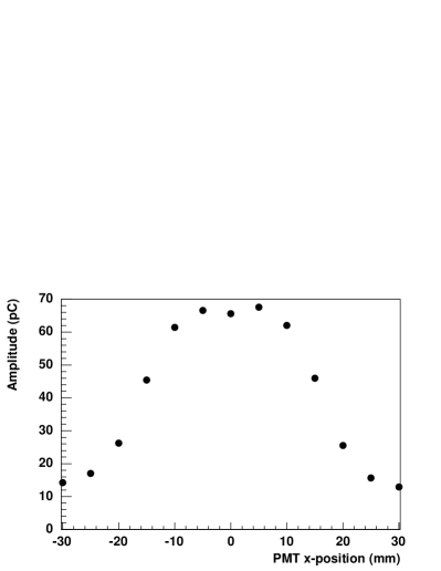
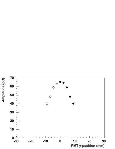
Figure 9: Measured signal time (top) and amplitude (bottom) as a function of horizontal and vertical aperture position. The width of the scintillator is 10 mm in y-direction and 32 mm in x-direction. Empty circles represent mirrored points.

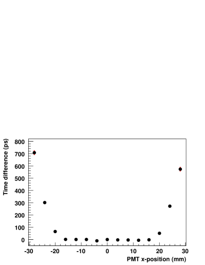
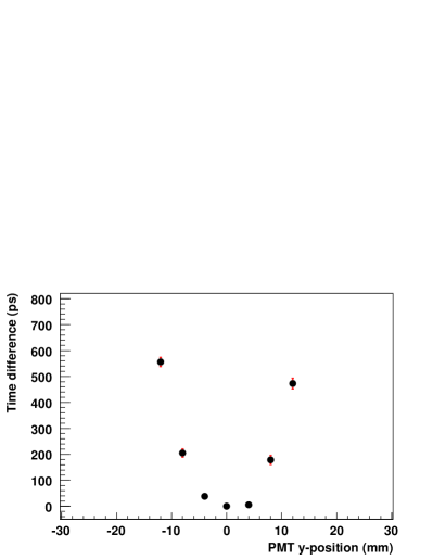
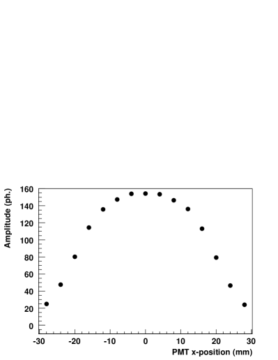
Figure 10: Simulated signal time (top) and amplitude (bottom) as a function of horizontal and vertical aperture position. The emission characteristics and the geometry of the scintillator have been adapted to the experiments.

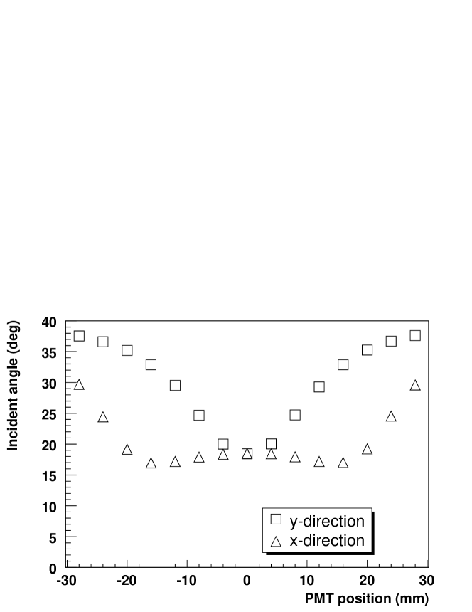
Figure 11: Simulated average photon angle with respect to the detection plane as a function of the horizontal and vertical aperture position. The emission characteristics and the geometry of the scintillator have been adapted to the experiments.

References

- [1] ANDA Collab., Strong interaction studies with antiprotons, Technical Progress Report, GSI, Darmstadt (2005).
- [2] COMPASS Collab., Outline for generalized parton distribution measurements with COMPASS at CERN, Expression of Interest CERN-SPSC-2005-007, CERN (2005).
- [3] G. Schepers, K. Götzen, J. Lühning, et al., Towards a DIRC-detector for the PANDA experiment, GSI Sci. Report 2005 FAIR-QCD-PANDA-05, p. 77, GSI, Darmstadt (2006).
- [4] N. Petrick, N. H. Clinthorne, W. L. Rogers, et al., First photoelectron timing error evaluation of a new scintillation detector model, IEEE Trans. Nucl. Sci. 38 (2) (1991) 174–177.
- [5] N. H. Clinthorne, N. A. Petrick, W. L. Rogers, et al., A fundamental limit on timing performance with scintillation detectors, IEEE Trans. Nucl. Sci. 37 (2) (1990) 658–663.
- [6] R. F. Post, L. I. Schiff, Statistical limitations on the resolving time of a scintillation counter, Phys. Rev. 80 (6) (1950) 1113.
- [7] F.-X. Gentit, Litrani: a general purpose Monte-Carlo program simulating light propagation in isotropic or anisotropic media, Nucl. Inst. & Meth. in Phys. Res. A486 (2002) 35–39.
- [8] D. Wahl, V. B. Mikhailik, H. Kraus, The Monte-Carlo refractive index matching technique for determining the input parameters for simulation of the light collection in scintillating crystals, Nucl. Inst. & Meth. in Phys. Res. A570 (2007) 529–535.
- [9] J. W. Nam, et al., A detailed Monte Carlo simulation for the Belle TOF system, Nucl. Inst. & Meth. in Phys. Res. A491 (2002) 54–68.
- [10] M. Moszyński, B. Bengtson, Status of timing with plastic scintillators, Nucl. Inst. & Meth. 158 (1979) 1–31.
- [11] Photomultiplier tubes: basics and applications, 2nd Edition, Hamamatsu (1999).
- [12] E. Shibamura, et al., Photon-to-electron conversion efficiency and reflectance of photomultiplier tubes as a function of incidence angle of photon, Nucl. Inst. & Meth. in Phys. Res. A567 (2006) 192–195.
- [13] P. Achenbach, J. Pochodzalla, S. Sánchez Majos, Measurement of photon angles for highly resolved TOF detectors, GSI Sci. Report 2005 FAIR-QCD-PANDA-04, p. 76, GSI, Darmstadt (2006).
- [14] N. H. Clinthorne, A. O. Hero III, N. A. Petrick, et al., Lower bounds on scintillation detector timing performance, Nucl. Inst. & Meth. in Phys. Res. A299 (1990) 157–161.