Characterization of the first true coaxial 18-fold segmented n-type prototype detector for the GERDA project

Abstract

The first true coaxial 18–fold segmented n–type HPGe prototype detector produced by Canberra–France for the GERDA neutrinoless double beta-decay project was tested both at Canberra–France and at the Max–Planck–Institut für Physik in Munich. The main characteristics of the detector are given and measurements concerning detector properties are described. A novel method to establish contacts between the crystal and a Kapton cable is presented.

, , , , , , , ,

1 Introduction

The GERmanium Detector Array, GERDA [1], is designed to search for neutrinoless double beta (0$\nu\beta\beta$)–decay of ⁷⁶Ge. The importance of such a search is emphasized by the evidence of a non-zero neutrino mass from flavor oscillations [2] and by the recent claim [3] based on data of the Heidelberg-Moscow experiment. GERDA will be installed in the Hall A of the Gran Sasso underground Laboratory (LNGS), Italy. The experiment is designed to collect an exposure of about 100$~{}kg\cdot y$ quasi background free. This leads to a requirement of a background index of better than 10^-3 counts/($kg\cdot y\cdot keV$) at the Q_ββ–value of 2039 $keV$. The main design feature of GERDA is to use a cryogenic liquid (Argon) as the shield against gamma radiation [4], the dominant background in earlier experiments [5]. High purity germanium detectors are immersed directly in the cryogenic liquid which also acts as the cooling medium. The cryogenic volume is surrounded by a buffer of ultra pure water acting as an additional gamma and neutron shield.

Customized segmented detectors are developed, because segmentation permits the identification of photon induced background events that have energy deposits at multiple locations (multi-site-events) over a centimeter scale. They are different from double-beta events which predominantely deposit energy at a single location (single-site-events) with a typical size of less than a few millimeters [6]. An 18–fold segmentation was chosen to optimize the identification of gamma induced background in the Q_ββ-region. The detector and its read-out cables were developed in collaboration between the Max–Planck–Institut für Physik, Munich, and Canberra–France, Lingolsheim. Canberra–France produced the detector. It was tested both at Canberra–France and at the MPI. The results presented here were all obtained operating the detector in a vacuum test–cryostat.

2 The Detector

The detector is n-type with an effective doping between $0.7\times 10^{10}/cm^{3}$ and $1.4\times 10^{10}/cm^{3}$ resulting in a full depletion voltage of about 2200 $V$. The standard operating voltage was set to 3000 $V$. The dimensions are 69.8 $mm$ in height and 75.0 $mm$ in diameter. The central bore has a diameter of 10.9 $mm$. The weight is 1.58 $kg$, the active volume is 302 $cm^{3}$ The geometry is true coaxial. The 18–fold segmentation is implemented as 6–fold in $\phi$ and 3–fold in $z$. The segmentation is created through a 3-d implantation process developed by Canberra–France. The most important detector parameters are listed in Tab. 1. The numbering of the segments as well as the definition of the coordinates are given in Fig. 1.

Parameter	Value
Nominal Operating Voltage	3000 $V$
Polarity	positive
Crystal Diameter	75 $mm$
Crystal Length	69.8 $mm$
Crystal Mass	1632 $g$
Active Volume	302 $cm^{3}$
FWHM at 122 $keV$	0.99 $keV$
FWHM at 1332 $keV$	1.99 $keV$
Relative Efficiency	80.4 %
Peak to Compton Ratio	75.5

Table 1: Delivery specifications of the first 18–fold segmented true coaxial prototype detector.

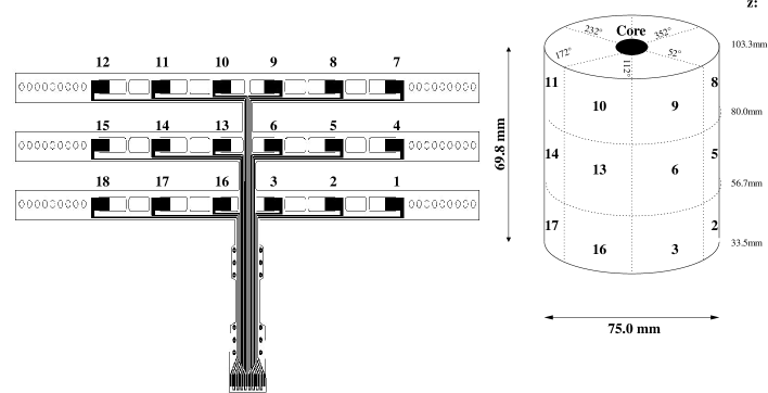
Figure 1: Left: Design of the Kapton board used to read out the signals of the individual segments. Right: Segmentation scheme of the detector including the coordinates used .

3 The Read-Out Cable with “Snap-Contacts”

The individual segments are read out using a Kapton printed-circuit-board (PCB). A schematic is given in Fig. 1. The contacts between detector segments and board are established with “snap-contacts”. The Kapton PCB is wrapped around the crystal with its copper traces on the outside. It has copper pads which are aligned with the contact pads of the detector and partially cut out. They are folded exposing half of their surface to the crystal pads. The Kapton board is tightened with a PTFE button that is plugged into the two appropriate holes of its two ends. The folded copper pads pressed onto the detector surface by the PCB form the snap-contacts.

Kapton and copper thicknesses of 50 $\mu m$ and 35 $\mu m$, respectively, were used for this first prototype. The tensile strength of the 35 $\mu m$ copper layer is essential for the reliability of the contact. A picture of a bare crystal with a Kapton board attached is shown in Fig. 2.

The snap-contacts establish contact without the introduction of any other materials. As there is no permanent attachment changing of cables is straight forward.

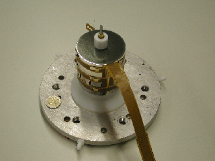
Figure 2: Ge crystal with the Kapton board wrapped around. The 18 segments are contacted with snap–contacts as described in the text.

4 The Test Environment

Tests were done both at Canberra–France and at the MPI. While the tests at Canberra–France focused on the basic functionality of the detector the measurements at the MPI targeted the performance with all segments read out simultaneously.

4.1 The Test Cryostat

A conventional aluminium vacuum test cryostat was used for all measurements. The detector with its Kapton cable and an appropriate high voltage contact was mounted inside and cooled through a copper cooling finger dipped into a conventional liquid nitrogen dewar.

The temperature at the top of the cooling finger (the closest point to the HPGe-crystal itself) was monitored using a PT100 inside the vacuum cap. Between daily refilling the temperature was stable between -171^o $C$ and -167^o $C$. Spectra within this temperature range were taken and compared with each other. Neither the energy resolutions nor the calibration parameters changed noticeably. The vacuum cryostat was pumped to a pressure of $10^{-6}~{}mbar$ before it was cooled down. The setup as mounted in Munich is depicted in Fig. 3.

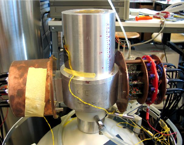
Figure 3: The test cryostat as mounted in Munich on top of a 30 $l$ liquid nitrogen dewar. The signals left the cryostat through two panels of feed-throughs and were amplified inside two copper “ears” housing 19 PSC 823 pre-amplifiers.

4.2 Cabling and Amplification

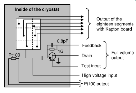
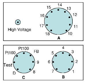
Figure 4: Left: Schematic drawing of the contacting scheme inside the test cryostat. Right: Assignment of the feed-throughs of the test cryostat. The high voltage and the signals of segments 10 to 18 were serviced on one side. The panel on the other side provided two feed-throughs for the signals from segments 1 to 9 as well as the drain [D], feedback [FB] and test line of the FET connected to the core inside the cryostat. In addition, the PT100 monitoring the temperature was read out through the multi-purpose connector C.

The test cryostat had two panels of feed-throughs opposite to each other. A schematic of the available lines and feed-throughs is given in Fig. 4. Two 7-channel feed-throughs were located on one side. Segments 1 to 9 as well as drain and feedback of the core signal plus the PT100 resistor were connected there. The signals of segments 10 to 18 were connected to a 9–channel connector on the panel on the opposite side. The high voltage input was serviced by a separate connector also located on this side.

The signals of the 18 segments were brought out of the cryostat without any amplification. Wires were soldered to the Kapton board and to the connectors. The signal of the core was pre-amplified by an FET inside the cryostat. All wires inside the cryostat were unshielded.

The signals were always amplified by PSC 823 pre-amplifiers produced by Canberra. At Canberra–France single channels were connected to a single pre-amplifier through a patch-panel. At the MPI all channels were connected simultaneously. Figure 3 shows the two copper housings called “ears” into which all 19 pre-amplifiers were integrated. The DC coupled room temperature FETs for the signals of the segments were sitting on the PC boards of the 18 pre-amplifiers themselves. The cold FET for the AC coupled core signal was sitting inside the detector cap and was thermally coupled to the cold finger.

It was of utmost importance to connect the pre-amplifiers to a very well defined common ground in order to avoid resonances and noise prohibiting the operation of the system. This was achieved through massive copper plates of 3 $~{}mm$ thickness inside the copper ears. All pre-amplifiers were directly connected to these plates. The plates were coupled to the aluminium-cap. Both the high voltage and the low voltages for the pre-amplifiers were filtered locally within the ears.

4.3 Data Aquisition

At Canberra–France a single channel data aquisition was used. The signals of the core or of any chosen segment were recorded as a histogrammed spectrum.

At the MPI a 75 MHz XIA Pixie–4 data acquisition system with 5 modules with 4 channels each integrated in a National Instruments crate was used. The pre-amplified signals were filtered and digitized [7]. The system has different modes of data storage. It can store energy spectra or for each event time and energy information or time and energy plus pulse shape information for each channel.

5 Basic Detector Properties

5.1 Full Depletion and Operational Voltage

The voltage dependence of the capacitance of the detector and its segments as well as of the leakage current were measured at Canberra–France. Figure 5 visualizes the results.

Figure 5: Voltage dependence of the leakage current (upper graph) and total capacitance (lower graph) of the detector.

The leakage current is constant in the voltage range between 1500 $V$ and 4000 $V$. Above 4000 $V$ the leakage current increases slightly with increased voltage. The detector capacitance decreases with increasing voltage until the value of 35 $pF$ is reached at full depletion around 2200 $V$. The standard operational voltage was set to 3000 $V$.

The individual segments have capacitances of around 2 $pF$ at full depletion. The values for the detector as a whole and for all individual segments at 3000 $V$ are listed in Tab. 2.

Segment	Capacitance	Resolution at 1.3 $MeV$
	[$pF$]	[$keV$]
total	34.88	4.07 $\pm$ 0.03
1	1.88	2.67 $\pm$ 0.05
2	1.91	2.63 $\pm$ 0.06
3	1.84	2.83 $\pm$ 0.05
4	1.92	2.53 $\pm$ 0.03
5	1.96	2.64 $\pm$ 0.04
6	1.89	3.36 $\pm$ 0.05
7	1.94	2.56 $\pm$ 0.02
8	1.96	2.28 $\pm$ 0.02
9	1.93	2.67 $\pm$ 0.02
10	2.01	3.99 $\pm$ 0.03
11	1.95	3.19 $\pm$ 0.03
12	1.98	2.93 $\pm$ 0.02
13	1.97	3.25 $\pm$ 0.01
14	1.94	2.50 $\pm$ 0.03
15	1.94	2.57 $\pm$ 0.03
16	1.94	2.81 $\pm$ 0.10
17	1.88	2.52 $\pm$ 0.05
18	1.97	2.79 $\pm$ 0.07

Table 2: Capacitance and energy resolution of each individual segment as well as for the total crystal (core in case of resolution). Capacitances were measured at Canberra-France, energy resolutions at the MPI in Munich.

5.2 Resolution

At Canberra–France the core resolution was determined from high statistics ⁵⁷Co and ⁶⁰Co calibration spectra. The measured FWHM resolutions were 0.99$~{}keV$ at 122$~{}keV$ and 1.99$~{}keV$ at 1.3$~{}MeV$, respectively (see Tab. 1).

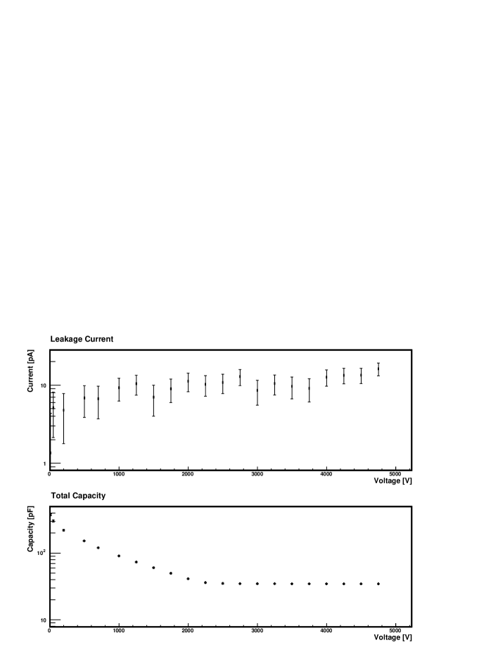
Figure 6: Peak area (left panel) and resolution (right panel) of the 1332.5 $keV$ ⁶⁰Co line as a function of the bias voltage. The energy resolution of the core was 3.1 $keV$ in this measurement eher not all segments were read out. In the later measurement referred to in Tab. 2 it was slightly worse.

At the MPI the voltage dependence of the core resolution was studied with a 60 $kBq$ ⁶⁰Co source located at a distance of 15 $cm$ to the side of the test cryostat. The segments were not read out for this test. Starting from 2000 $V$ spectra were taken at voltage steps of 100 $V$. Each measurement lasted 10 minutes. The 1.3 $MeV$ line was used for the analysis. For each spectrum a Gaussian plus a constant background was fitted and the number of counts within the peak as well as the FWHM were calculated. The results are shown in Fig. 6. The energy resolution decreases as the count rate increases until full depletion is reached.

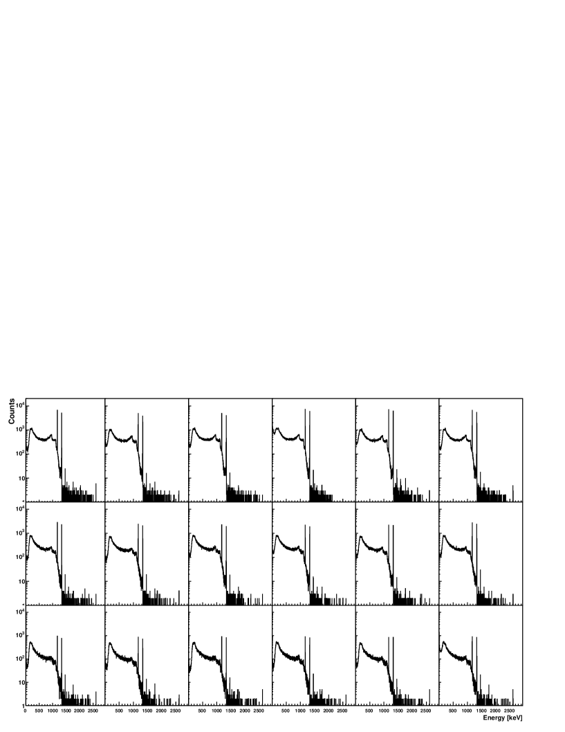
Figure 7: ⁶⁰Co spectra of all 18 segments when read out simultaneously. The arrangement of the graphs is such that the spectra of the 6 upper segments are displayed on top, the 6 lower at the bottom. The spectra shown are corrected for cross-talk (see section 6.2).

The 60 $kBq$ ⁶⁰Co source was also used to determine the resolution of all segments while they were read out simultaneously. The source was placed 5 $cm$ above the center of the test cryostat. The measurement lasted 30 minutes. The pulse heights of the core and all segments were recorded for each event. Only events with core energy bigger than 20 $keV$ were used. The resulting energy spectra of the individual segments are shown in Fig. 7. The arrangement of the spectra in Fig. 7 is according to the physical location of the segments on the detector as depicted in Fig. 1. The upper six spectra correspond to the upper six segments of the crystal and thus were closest to the calibration source. This is reflected in the higher statistics in the spectra of these segments.

Fits as described above applied to the 1.3$\,MeV$ peak were used to determine the energy resolution of the individual segments. The results are listed in Tab. 2. The segment resolutions range between 2.3 $keV$ and 4.0 $keV$. The core resolution for this measurement was 4.1 $keV$. This value of the resolution is worse than the one observed in the measurement described in a previous paragraph where the segments were not read out. This is due to interference between the experimental surrounding and the electronics channels.

In general the resolutions were not exactly reproducable. They varied between 2 $keV$ and 5 $keV$. As mentioned before the performance of the pre-amplifiers was extremely dependent on the quality of the grounding. Even the tightness of the screws closing the ears was seen to change the resolution by the order of one keV. In addition, the setup was exposed to varying electromagnetic noise caused by machinery in neighbouring laboratories. The resolutions were definetly not limited by detector properties, but by the limitations of screening and grounding.

6 Data Quality

6.1 Linearity

The linearity of the response of the system was tested with lines distributed between 350 $keV$ and 2614.53 $keV$. The list of lines is given in Tab. 3. The lines of ⁶⁰Co were augmented by several lines of the background seen in the laboratory.

Energy [$keV$]	Element
351.92 $keV$	214Bi	background
609.31 $keV$	214Bi	background
661.66 $keV$	137Cs	background
1173.24 $keV$	60Co	source
1332.5 $keV$,	60Co	source
2505.74 $keV$	60Co	source
1460.81 $keV$	40K	background
2614.53 $keV$	208Tl	background

Table 3: The lines used to study the linearity of the read-out system.

The peaks in the core spectra were fitted with the usual procedure. The extent of the linearity can be seen in Fig. 8. The energy response function is plotted in the left panel. The right panel shows the residuals between the linear fit function and the data points.

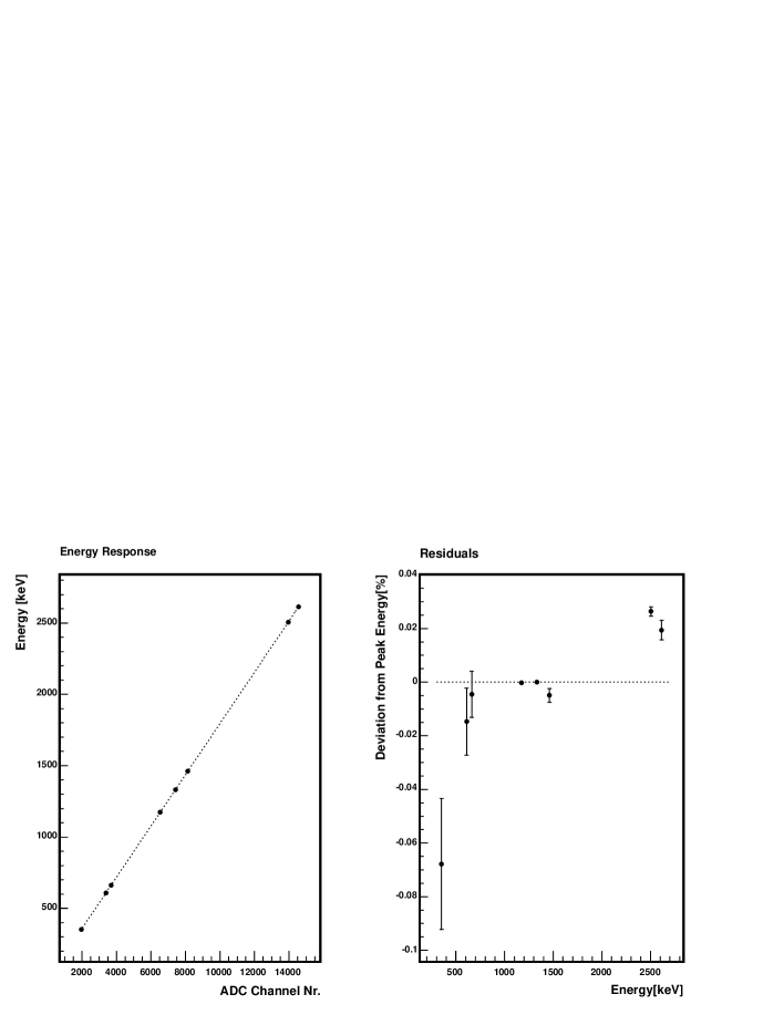
Figure 8: Energy calibration of the core signal using peaks from a ⁶⁰Co source and background. The left panel shows the energy response function. The right panel gives the residuals to the linear fit function depicted in the left panel.

6.2 Cross-Talk

Events taken with a ²²⁸Th source were used to study the cross-talk between read-out channels. In the left panel of Fig. 9 a scatter plot of the energy seen in the core vs. the energy in segment 1 is shown. Each dot corresponds to one event. The diagonal which corresponds to the single segment events with all the energy deposited in segment 1 is clearly visible. Entries above this diagonal are physically not allowed since this would mean that the energy deposited inside a single segment is larger than in the whole detector. The core events that did not deposit any energy in segment 1 are expected to lie on the x-axis provided there is no cross-talk. In Fig. 9 they are shifted to a line with a non-vanishing positive slope. This is due to cross-talk from the core into segment 1. This is actually expected, since the FET for the core signal is located inside the aluminium cap. Any amplified signal from the core is thus going through the same feedthrough as the unamplified signals from segments 1 to 9. This leads to a pick-up in these channels.

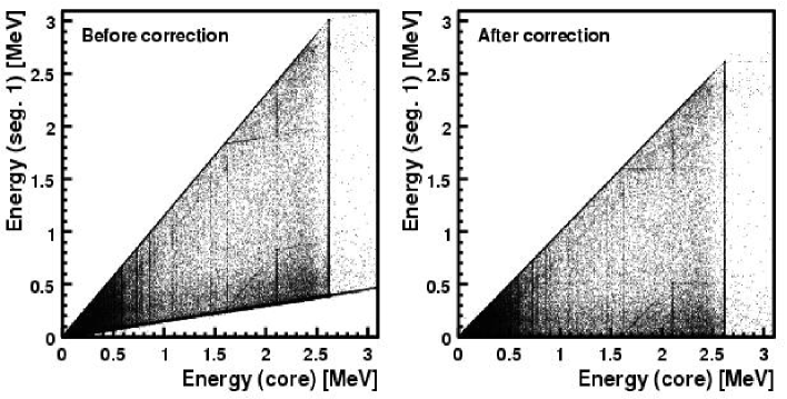
Figure 9: Scatter plots of the energy seen by the core [x-axis] vs. the energy seen by segment 1 [y-axis]. Each dot corresponds to one event. Left panel: Uncorrected data. The cross talk between the signal in the core and in segment 1 is seen as the slope of the line below which there are no entries. The events with no energy deposited in segment 1 still show an effective signal. Right panel: Scatter plot of the same data as displayed in left panel, but after cross-talk correction.

The observed cross-talk can easily be corrected for. Neglecting second order effects the true energy deposition in a segment E_seg,true can be calculated as

$$E_{seg,true}=E_{seg,meas}-\kappa_{seg}E_{core},$$ (1)

where E_seg,meas and E_core are the measured values for the segment and core respectively. The factor $\kappa_{seg}$ is a correction factor to be determined for each individual segment. Tab. 4 lists the coefficients for the affected segments. The cross-talk seen for channels 1 to 9 varies between 1 $\%$ and 38 $\%$, being the strongest for segment 9. The right plot of Fig. 9 visualizes the same data as the left plot after the application of the cross-talk correction.

Segment	1	2	3	4	5	6	7	8	9
$\kappa_{seg}$	0.128	0.014	0.009	0.033	0.024	0.037	0.014	0.037	0.385

Table 4: Cross-talk coefficients $\kappa_{seg}$ of segments 1 to 9. Cross talk from the core signal is seen for the segments that have their signal feed-through on the same side as the amplified core signal. No cross-talk is observed for segments 10 to 18.

The quality of the correction can be deduced from Fig. 10. The projection of the scatter plot of the right panel of Fig. 9 onto the y–axis is shown for events with a measured core energy of more than 1750 $keV$. This projection shows the corrected energy in segment 1 which should be distributed around 0 $keV$ for the selected events.

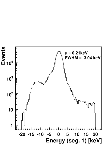
Figure 10: Projection of core events with E $\geq$ 1750 $keV$ onto segment 1 energy after correction. The same data set as in Fig.9 has been used. For interpretation see text.

A perfect correction would result in only one Gaussian peak centered exactly at 0 $keV$. The width would be determined only by the electronics and the DAQ. In Fig. 10 a Gaussian was fitted for the interval -3 $keV$ to +3 $~{}keV$. It peaks at (0.207 $\pm$ 0.002) $keV$ and results in a FWHM resolution of (3.04 $\pm$ 0.01) $keV$. There are second order effects which result in distortions of the Gaussian. However, they are quite small and do not need to be corrected for. Please note the logarithmic scale.

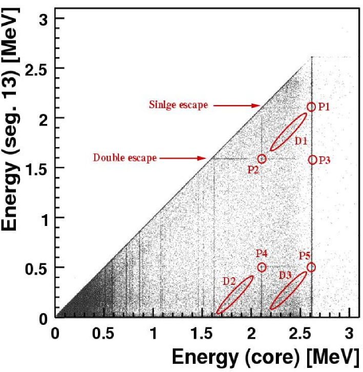
Figure 11: Scatter plot of the core energy vs. energy in segment 13. Each dot corresponds to one event. Cross-talk is not observed in segment 13. The marked structures are discussed in sect. 7 in the text.

The segments 10 to 18 are not affected by cross-talk from the core. Their feed-throughs are on the other side of the cryostat. This is demonstarted in Fig. 11 where an uncorrected scatter plot is shown for the energy seen by the core vs. the energy seen in segment 13. The cross-talk between segments is insignificant and not taken into account.

7 Segment Spectra Correlations

Several well understood features appear in the segment 13 scatter plot depicted in Fig. 11. The ²²⁸Th source used has a number of strong gamma lines. The vertical lines clearly visible in the plot are caused by events in which all the energy of a photon is deposited within the crystal while only part of this energy is deposited in segment 13.

Photons from the 2615 $keV$ line are responsible for several features marked in Fig. 11. Photons of this energy are likely to loose their energy via pair production (see for example [8]). The created electron will be stopped locally, i.e. with high probability within one segment. The positron will also be stopped locally and annihilate. Two 511 $keV$ gammas are emitted in this process. The horizontal lines are due to one ore both 511 $keV$ gammas escaping the segment but still depositing some energy in the crystal before escaping it.

The marked areas correspond to the following pair-production (pp) scenarios:

1. pp in segment 13. One 511 $keV$ gamma escapes the segment, but is absorbed elsewhere in the crystal.

2. pp in segment 13. Both 511 $keV$ gammas escape the segment. One deposits its total energy elsewhere in the crystal, the second escapes the crystal.

3. pp in segment 13. Both 511 $keV$ gammas escape the crystal.

4. pp in segment 13. One 511 $keV$ escapes segment 13 and deposits its full energy inside the crystal. The other $keV$ gamma deposits some of its energy in segment 13 and escapes the ctrystal.

5. pp inside a segment other than segment 13. One 511 keV gamma leaves the crystal without depositing any energy. The other deposits its total energy in segment 13.

6. pp inside a segment other than segment 13. All 2615 $keV$ are deposited in the crystal. One 511 $keV$ gamma deposits its total energy in segment 13.

7. pp inside a segment other than segment 13. One 511 $keV$ gamma escapes the crystal. The second one deposits some of its energy in segment 13 before escaping the crystal.

8. pp inside a segment other than segment 13. One annihilation gamma deposits some of its energy within segment 13 before escaping the crystal. The other gamma deposits all its energy elsewhere in the crystal.

8 Detector Characterization

8.1 Segment Boundaries

The location of the segment boundaries were determined using the 122 $keV$ line of a collimated ¹⁵²Eu source which was moved along $z$ and $\phi$. Since the main energy loss mechanism in germanium at the energy of 122 $keV$ is the photo-effect [8] and the mean free path is roughly 4 $mm$, the energy of the photon is deposited predominantly locally. Segment 14, not affected by cross-talk, was chosen to be in the center of the test area. Its center was found to be at $z=68.4$ $mm$ and $\phi=202^{\circ}$. From the center the source was moved in steps of 5 $mm$ in $z$ and 5^∘ in $\phi$. The spectra were taken for each measurement and the pulse-shapes of all events were recorded.

The average count rate in the 122 $keV$ peak was calculated for segment 14 and its neighbours for each measurement. The result is shown in Fig. 12. The count rates peak whenever the source is placed above the physical center of a segment. The shape of the count rate distribution can be described by the convolution of a Gaussian representing the width of the beam-spot and a box function representing the borders of the segments. The distances between maxima were constrained to the known physical distances between segment centers (23.3 $mm$ in $z$, 60^∘ in $\phi$). In Fig. 12 the results of the fits are shown for each segment. As it is determined by the source, the size of the beam-spot shoud be constant throughout the measurements. The widths of the Gaussian functions as fitted are given in Tab. 5. The numbers are consistent within errors. The maxima as seen in Fig. 12 can be different for each segment since the geometry of the aluminium cap as well as the Kapton PC-board on the segment do slightly differ between segments.

	Height	Width
Segment	FWHM	FWHM
11	(5.9 $\pm$ 0.8) $mm$	–
13	–	(12.3 $\pm$ 0.5)o
14	(5.6 $\pm$ 0.6) $mm$	(12.0 $\pm$ 0.5)o
15	–	(13.3 $\pm$ 0.7)o
17	(6.1 $\pm$ 0.7) $mm$	–

Table 5: Size of the beam spot of the ¹⁵²Eu source as determined from the data used to scan the segment boundaries. Within the errors the size stays constant throughout the measurements.

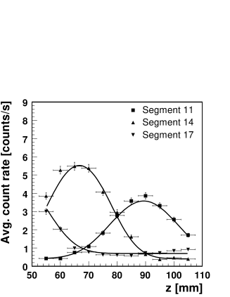
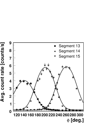
Figure 12: Average count rates in dependence of the $z$ [left] and $\phi$ [right] position of the ¹⁵²Eu source.

8.2 Crystal Axes

The propagation of electrons and holes in the electric field of the germanium crystal is influenced by the crystal axes[9]. The charge carriers get deflected and do not follow a simple radial path. Thus, the time to collect the charge depends on the angle between the closest crystal axis and the radial line on which the interaction takes place. This is reflected in the rise-times of the pulses recorded. The pulse-shapes of all events used in the previous section were recorded. The ¹⁵²Eu scan along the azimuthal angle $\phi$ was analyzed with respect to the average 10 $\%$ to 30 $\%$ and 10 $\%$ to 90 $\%$ rise-times of the pulses. The results are shown in Fig. 13. The distribution of average rise-times clearly varies with $\phi$. The distance between the extrema is 90^o as expected. The positions of the extrema clearly establish the orientation of the crystal axes.

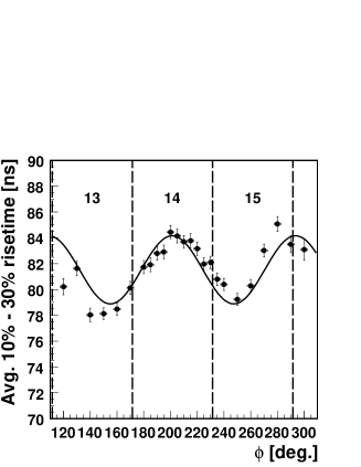
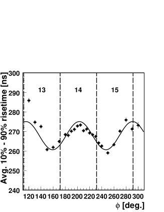
Figure 13: Average 10 $\%$ to 30 $\%$ (left panel) and 10 $\%$ to 90 $\%$ (right panel) rise-times as a function of the azimuthal angle $\phi$. The average rise-times were calculated from pulses in the 122 $keV$ line of ¹⁵²Eu in which the energy is deposited very close to the surface.

8.3 Radius Dependence of the Rise-Time

In the previous section interactions close to the outer surface of the detector were used. In order to study dependence of the rise-time on the radius of the interaction point the source was placed above the detector and moved along the center-line of segment 11 along $r$. The end of the collimator with the ¹⁵²Eu source was positioned 5 $mm$ above the aluminium cryostat. Starting at $r=5$ $mm$ data was taken with a step-size of 5 $mm$ in $r$. The pulses in the 122 $keV$ peak were used to calculate the average rise-times for segment 11 and the core at each interaction point. Fig. 14 shows a clear correlation between rise-time and radius $r$.

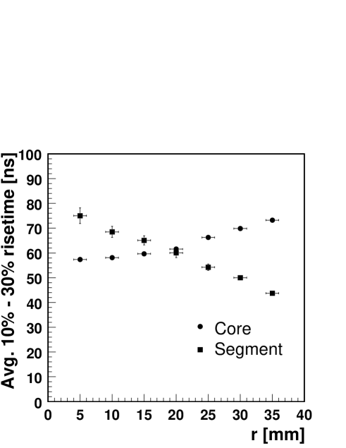
Figure 14: Average 10 $\%$ to 30 $\%$ rise-time as a function of the radius of the interaction point for events in the 122 $keV$ peak of ¹⁵²Eu.

The 10 $\%$ to 30 $\%$ rise-time was chosen because this separates between electrons and holes. The average rise-time of the pulses from the core increases not strictly linear with the radius. At small radii the dependence is very small. The dependence of the average rise-time of the pulses from the segment shows a larger dependence on the radius which, in addition, remains linear throughout the crystal. The rise-time of the segment pulses can thus be used to deduce information about the depth of interactions.

8.4 Mirror charge asymmetry

The electron-hole pairs created in the volume of a given segment create mirror charges in the neighboring segments. This phenomenon can be understood and deducted from Ramo’s theorem (see for example [10]). The amplitude of the induced mirror-charge-pulse depends on the distance between the interaction point and the boundary between the irradiated segment and the segment under consideration: the smaller the distance the larger the mirror charge. Mirror-charge amplitude asymmetries are defined for the neighboring segments opposite to each other:

$$A_{rl}=log_{10}(A(13)/A(15))~{}~{}~{}\mathrm{and}~{}~{}~{}A_{tb}=log_{10}(A(11)/A(17)).$$ (2)

The same data set as in the section 8.1 was used. Only pulses in the 122 $keV$ peak were used in order to select events with mostly only one interaction.

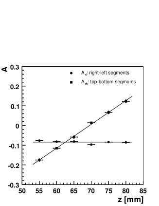
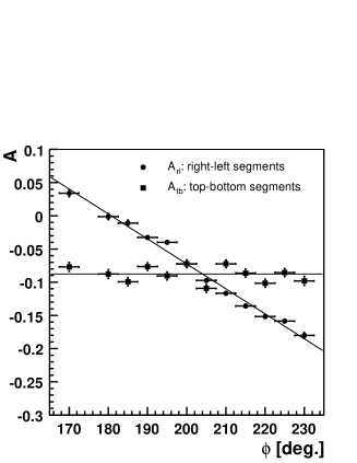
Figure 15: Asymmetries between mirror-charge amplitudes of segments neighboring the irradiated one as a function of $z$ (left panel) and $\phi$ (right panel). The events in the 122 $keV$ peak of ¹⁵²Eu were used to calculate the asymmetries A from equation 2. For the definitions of A and further details see the text.

In Fig. 15 the mean values of A_rl and A_tb are shown for source position as a function of z and $\phi$. In the left panel the measured average asymmetries are shown for the z-scan. The asymmetry of the neighbors left and right from the irradiated segment (14) is not altered with changing z since the mean distance between the segment borders does remain the same for all measurements. As expected the average asymmetry between neighbors below and above the irradiated segment does however show a clear dependence on z. The difference of the mirror charge amplitudes on segments 11 and 17 is the largest for the measurements closest to their boundary. As shown in the right panel of Fig. 15 the predicted behavior is also reproduced from the $\phi$-scan.

8.5 Position Resolution

If the mirror-charge amplitude asymmetry distributions are known, the $z$- and $\phi$-coordinates of the interaction point can be obtained for single-site events. The precision obtained is 6 $mm$ in $z$ and about 13^∘ in $\phi$. It is dominated by the beam spot size.

Additionally, the radius can be obtained from the radius dependence of the rise time as shown in Fig. 13. The resolutions is about 5 $mm$.

9 Photon Identification

The ability to identify photon induced events was studied in detail with several sources. A detailed analysis is presented in [11].

Here, only a core spectrum taken with a ⁶⁰Co source 5 $cm$ above the crystal is shown. Also shown in Fig. 16 is the reduction of the spectrum, if it is required that only one segment has an energy deposition above 20 $keV$. At around 2 MeV about 90 % of the events are rejected. The summation peak of the 1173.2 $keV$ and 1332.5 $keV~{}^{60}$Co lines at 2505.7 $keV$ is almost completely suppressed in the anti-coincidence spectrum. This is due to the fact that it is very unlikely for the two photons to deposit their full energy in the same segment.

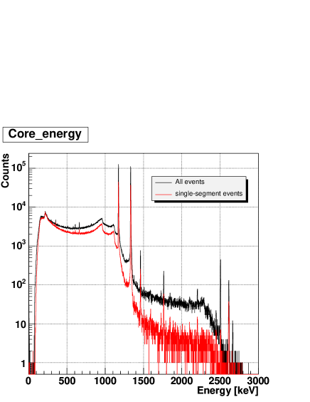
Figure 16: Core spectrum of a ⁶⁰Co source placed 5 cm above the crystal. The black histogram shows the total core spectrum, the red one the spectrum of single segment events. The reduction of the Compton-background at 2 $MeV$ is roughly a factor of 10.

10 Conclusion

The first 18–fold segmented true coaxial n-type HPGe detector developed and produced by Canberra-France, Lingolsheim, worked according to specifications within a conventional test cryostat.

A novel low-mass contacting scheme was developed and tested. The copper pads of a Kapton PC-board were shaped into snap-contacts which contact the crystal pads without any additional material. The contacts performed reliably during the tests.

The energy resolutions (FWHM) between 2 $keV$ and 4 $keV$ for core and segments were limited by the grounding and screening of the test electronics. Crystal axes were determined as well as the radial dependence of the rise-time of the pulses. The reconstruction of the position of a single interaction was investigated as well as the identification of photons with the help of segment anti-coincidences. The results confirmed the expectations.

References

- [1] S. Schönert et al. [GERDA Collaboration], Nucl. Phys. Proc. Suppl. 145 (2005) 242.
- [2] Particle Data Group, Journal of Phys. G 33 (2006)483
- [3] H.V. Klapdor-Kleingrothaus et al., “Data acquisition and Analysis of the 76Ge double beta experiment in Gran Sasso 1990-2003”, Nucl. Instr. Meth. A 522(2004)371-406
- [4] G. Heusser, “Low-Radioactivity Background Techniques”, Annu. Rev. Nucl. Part. Sci. 45(1995)543
- [5] C. Dörr and H.V. Klapdor-Kleingrothaus, “New Monte-Carlo simulation of the HEIDELBERG-MOSCOW double beta decay experiment”, Nucl. Instr. Meth. A 513(2003)596
- [6] I. Abt et al., “Background suppression in neutrinoless double-beta decay experiments using segmented detectors - a Monte Carlo study for the GERDA setup”, Nucl Instr. Meth. A 570(2007)479
- [7] “Digital Gamma Finder (DGF) PIXIE-4”, User’s manual. X-Ray Instrumentation Associates, http://www.xia.com
- [8] G.F. Knoll, “Radiation Detection and Measurement”, 3rd edition, J. Wiley Sons, Inc.,2000
- [9] H. G. Reik and H. Risken, Phys. Rev. 126 (1962) 1737-1746
- [10] Z. He, “Review of the Shockley-Ramo theorem and its application in semiconductor gamma-ray detectors”, Nucl. Instr. Meth. A 463(2001) 250-267
- [11] I. Abt. et al, “Identification of photons in double beta decay experiments using segmented germanium detectors - studies with a GERDA Phase II prototype detector”, to be published, nucl-ex/0701005.