Polarization of Hyperons in Elementary Photoproduction

Abstract

Recent measurements using the CLAS detector at Jefferson Lab of the reactions $\vec{\gamma}+p\to K^{+}+\vec{\Lambda}$ and $\vec{\gamma}+p\to K^{+}+\vec{\Sigma}^{0}$ have been used to extract the spin transfer coefficients $C_{x}$ and $C_{z}$ for the first time. These observables quantify the degree of the photon circular polarization that is transferred to the recoiling hyperons in the scattering plane. The unexpected result is that $\Lambda$ hyperons are produced “100% polarized” as seen when combining $C_{x}$ and $C_{z}$ with the induced transverse polarization, $P$. Furthermore, $C_{x}$ and $C_{z}$ seem to be linearly related. This paper discusses the experimental results and offers a hypothesis which can explain these observations. We show how the produced strange quark can be subject to a pure spin-orbit type of interaction which preserves its state of polarization throughout the hadronization process.

1 Introduction

At the HYP2006 Conference in Mainz in October 2006 I presented a talk entitled “Experiments with Strangeness in Hall B at Jefferson Lab.” There were two topics: first, the measurement of the spin transfer coefficients $C_{x}$ and $C_{z}$ in $K^{+}Y$ production off the proton using real photons bradford , and second, the measurement of four separated cross section components in $K^{+}Y$ electroproduction ambrozewicz . Both topics are the subjects of long papers that have since been submitted for publication, as cited, and essentially all points made in the talk are covered in those two papers.

Rather than repeat that discussion, this paper will provide further details about the $C_{x}$ and $C_{z}$ spin transfer work that were partly mentioned in the talk, but not covered in Ref. bradford . Two phenomenological puzzles were presented in the talk and the paper regarding the new polarization observables. First, the magnitude of the $\Lambda$ polarization vector, $|\vec{P}_{\Lambda}|$, comprised of three measured orthogonal components, is unity at all production angles and for all center of mass (c.m.) energies $W$. For a fully polarized photon beam, $\vec{P}_{\Lambda}$ is equivalent to a quantity we introduce called $\vec{R}$, defined as $\vec{R}=C_{x}\hat{x}+P\hat{y}+C_{z}\hat{z}$. The component $P$ is the induced or transverse polarization, using the notation common in the literature for this quantity. We find $|\vec{R}|=\sqrt{C_{x}^{2}+C_{z}^{2}+P^{2}}=1$ to very good precision. Second, there appears to be a simple linear relationship between the two spin transfer coefficients, to wit, $C_{z}=C_{x}+1$. Both of these observation may be considered quite unexpected since there is no a priori reason for the $\Lambda$ hyperon polarization to be $100\%$, nor is there an obvious relationship among the production amplitudes discussed in the literature to lead to this result. Indeed, no present theoretical models incorporates these new pieces of phenomenology. In this paper I present a somewhat heuristic model, or hypothesis, which can explain these findings and which may be a foundation for additional theoretical work.

2 Methods, Formalism and Results

2.1 Measurement Method

An energy-tagged real photon beam was created in the Hall-B beam line at Jefferson Lab between energies corresponding to the hyperon production threshold near $W=1.679$ GeV and 2.454 GeV. The electron beams that created the photons via bremsstrahlung were longitudinally polarized at about $65\%$, for beam energies at 2.4 and 2.9 GeV. This longitudinal polarization was transferred as circular polarization of the created photons during in a well-defined way during bremsstrahlung, with maximum transfer at the endpoints. An unpolarized 18 cm long liquid hydrogen target was used. The CLAS detector was triggered by any single charged-particle track, including pions, kaons, and protons. For this analysis, a positive kaon track and a proton track from hyperon decay were required to be present, but the $\pi^{-}$ from the hyperon decay was not used. Differential cross sections and the induced recoil polarization $P$ from this experiment were published previously mcnabb .

Figure 1 shows our axis convention. In the c.m. frame we adopt the $\{\hat{x}$, $\hat{y}$, $\hat{z}\}$ system wherein the $\hat{z}$ axis points along the photon direction; it is the most natural one in which to present these results. The $\Lambda$ hyperon is produced polarized, and we can measure the components of this polarization using the parity-violating weak decay asymmetry of the protons (or pions) in the rest frame of the $\Lambda$, as illustrated in the dotted box. All three components of the polarization can be extracted by projecting along the relevant axes. In the specified coordinate system $i\in\{x,y,z\}$ is one of the three axes. The decay distribution, $I_{i}(\cos\theta_{i})$, is given by

$$I_{i}(\cos\theta_{i})={\textstyle\frac{1}{2}}(1+\nu\alpha P_{Yi}\cos\theta_{i}),$$ (1)

where $\theta_{i}$ is the proton polar angle with respect to the given axis in the hyperon rest frame. The weak decay asymmetry, $\alpha$, is taken to be $0.642$. The factor $\nu$ is a “dilution” arising in the $\Sigma^{0}$ case due to its radiative decay to a $\Lambda$, and which is equal to $-1/3$ in the $\Lambda$ rest frame. A complication arose for us because we measured the proton angular distribution in the rest frame of the parent $\Sigma^{0}$. This led to a value of $\nu=-1/3.90$, as discussed in Ref. bradford . For the $K^{+}\Lambda$ analysis $\nu=+1.0$. Extraction of $P_{Yi}$ follows from fitting the linear relationship of $I_{i}(\cos\theta_{i})$ vs. $\cos\theta_{i}$. The polarization of the hyperon in the c.m. frame is the same as it is in the hyperon rest frame in this experiment: there is no Wigner rotation when boosting from the hyperon rest frame to the c.m. frame bradford .

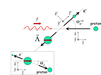
Figure 1: In the overall reaction center of mass, the coordinate system can be oriented along the outgoing $K^{+}$ meson $\{\hat{x}^{\prime},\hat{y}^{\prime},\hat{z}^{\prime}\}$ or along the incident photon direction $\{\hat{x},\hat{y},\hat{z}\}$. The dotted box represents the rest frame of the hyperon, and the coordinate system used for specifying the polarization components. The short heavy arrows represent polarization vectors.

Let $P_{\odot}$ represent the degree of beam polarization between $-1.0$ and $+1.0$. Then the spin-dependent cross section for $K^{+}Y$ photoproduction can be expressed as barker

$$\rho_{Y}\frac{d\sigma}{d\Omega_{K^{+}}}=\left.{\frac{d\sigma}{d\Omega_{K^{+}}}}\right|_{unpol.}\!\!\!\!\!\!\!\!\!\!\!\left\{1+\sigma_{y}P+P_{\odot}(C_{x}\sigma_{x}+C_{z}\sigma_{z})\right\}.$$ (2)

Here $\rho_{Y}$ is twice the density matrix of the ensemble of recoiling hyperons $Y$ and is written

$$\rho_{Y}=(1+\vec{\sigma}\cdot\vec{P}_{Y}),$$ (3)

where $\vec{\sigma}$ are the Pauli spin matrices and $\vec{P}_{Y}$ is the measured polarization of the recoiling hyperons. In Eq. 2 the spin observables are the induced polarization $P$, and the polarization transfer coefficients $C_{x}$ and $C_{z}$.

We define our $C_{x}$ and $C_{z}$ with signs opposite to the version of Eq. 2 given in Ref. barker . This makes $C_{z}$ positive when the $\hat{z}$ and $\hat{z}^{\prime}$ axes coincide at the forward meson production angle, meaning that positive photon helicity results in positive hyperon polarization along $\hat{z}$.

The connection between the measured hyperon recoil polarization vector $\vec{P}_{Y}$ and the spin correlation observables $P$, $C_{x}$, and $C_{z}$, is obtained by taking the expectation value of the spin operator $\vec{\sigma}$ with the density matrix $\rho_{Y}$ via the trace: $\vec{P}_{Y}=Tr(\rho_{Y}\vec{\sigma})$. This leads to the identifications

$$P_{Yx} = P_{\odot}C_{x}$$ (4)

$$P_{Yy} = P$$ (5)

$$P_{Yz} = P_{\odot}C_{z}.$$ (6)

The transverse or induced polarization of the hyperon, $P_{Yy}$, is equivalent to the observable $P$, while the $\hat{x}$ and $\hat{z}$ components of the hyperon polarization are proportional to $C_{x}$ and $C_{z}$ via the beam polarization factor $P_{\odot}$. Physically, $C_{x}$ and $C_{z}$ measure the transfer of circular polarization, or helicity, of the incident photon on an unpolarized target to the produced hyperon.

To extract $C_{x}$ and $C_{z}$ the beam helicity asymmetry $A_{i}$ was accumulated in each bin of proton decay angle with respect to the $\hat{x}$ or $\hat{z}$ axis, and a fit to this asymmetry as a function of $\cos\theta_{i}$ was made. $C_{i}$ was computed from

$$A(\cos\theta_{i})=\frac{N_{+}-N_{-}}{N_{+}+N_{-}}=\alpha\nu P_{\odot}C_{i}\cos\theta_{i}.$$ (7)

where $N_{\pm}$ are the helicity-dependent yields in each bin. The overall systematic uncertainty for the $K^{+}\Lambda$ results was $\pm 0.03$ for $\cos\theta^{c.m.}_{K^{+}}<0.55$ and $\pm 0.09$ for $\cos\theta^{c.m.}_{K^{+}}>0.55$. The total global systematic uncertainty for the $K^{+}\Sigma^{0}$ results as $\pm 0.03$ for $\cos\theta^{c.m.}_{K^{+}}<0.35$ and $\pm 0.17$ for $\cos\theta^{c.m.}_{K^{+}}>0.35$. The systematic uncertainty in $W$ was $\pm 2$ MeV at the bin centers. More thorough discussion of the experimental and analysis details can be found in Ref. bradford .

2.2 Experimental Results

Values of $C_{x}$ and $C_{z}$ in their smallest binning of $W$ and $\cos\theta_{K^{+}}^{c.m.}$ are presented in Ref. bradford . Also shown is that the values of

$$|\vec{R}_{\Lambda}|\equiv\sqrt{P^{2}+C_{x}^{2}+C_{z}^{2}}$$ (8)

in all bins are remarkably close to unity for the $\Lambda$. To emphasize this more clearly in the present paper, in Fig. 2 we show the effect of averaging those results for the $|\vec{R}_{\Lambda}|$ across all values of $W$ and showing the results as a function of kaon production angle (top panel), or averaging over all angles and showing the results as a function of $W$. The points are the weighted mean of the data. The inner error bars on each point correspond to the uncertainty on the weighted mean of the data. However, taking a weighted mean is strictly appropriate only if one knows that the set of values to be combined measure the same physical quantity. This experiment has discovered that the values seem to be consistent with unity, but a more fair way of representing the spread of these values, absent certain knowledge that they should be the same, is to use the weighted variance. The latter is shown as the outer error bars on the points. Some data points lie above unity by about one full error bar, but this is to be expected based on the analysis method and random error statistics: the fitted asymmetries were not biased by imposition of the physical limit at $R=+1.0$.

The unexpected observation is that across all measured angles and energies the value of $|\vec{R}_{\Lambda}|$ is consistent with unity. Taking the grand weighted mean over the results at all energies and angles we find

$$\overline{R}_{\Lambda}=1.01\pm 0.01,$$ (9)

where the uncertainty is that of the weighted mean. Our systematic uncertainty is about $\pm 0.03$. The $\chi^{2}$ for a fit to the hypothesis that $|\vec{R}_{\Lambda}|=1$ is 145 for 123 degrees of freedom, for a reduced chi-square of 1.18, which is a good fit. One may therefore conclude that the $\Lambda$ hyperons produced in $\vec{\gamma}+p\to K^{+}+\vec{\Lambda}$ with circularly polarized photons appear 100% spin polarized. This result is only “natural” at extreme forward and backward angles where the $K^{+}\Lambda$ final state system has no orbital angular momentum available, and all of the photons’ helicity must end up carried by the hyperon. Since this situation is not required by the kinematics of the reaction, there must be some dynamical origin of this phenomenon, as discussed below.

Shown in Ref. bradford is that $C_{z}$ is large and positive over most of the kinematic range, except at back angles where considerable “resonance-like” fluctuations are seen. The observable $C_{x}$ has similar fluctuations as $C_{z}$ but is typically smaller by one full unit, meaning that to a good approximation

$$C_{z}\simeq C_{x}+1.$$ (10)

This is the second unexpected observation about the results of this experiment. Taking the weighted mean of the difference $D\equiv C_{z}-C_{x}-1$ over all values of $W$ and kaon angle leads to the value

$$\overline{D}=0.054\pm 0.012$$ (11)

In this case the $\chi^{2}$ for a fit to the hypothesis of Eq. 10 is 306 for 159 degrees of freedom, or 1.92 for the reduced $\chi^{2}$. This is a poor fit, so our confidence in the accuracy of this simple empirical relationship is limited, and indicates that it needs experimental confirmation. Nevertheless, we offer a possible reason for this relationship below.

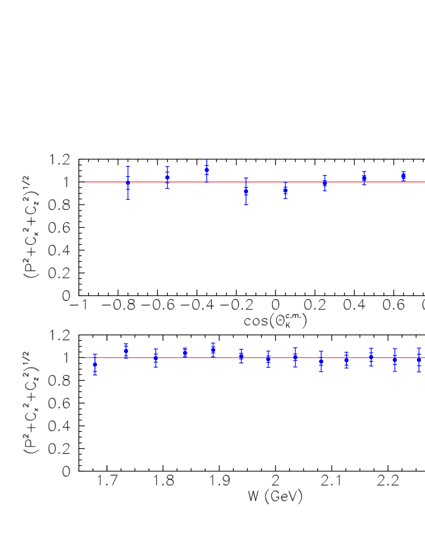
Figure 2: Magnitude of the polarization of the $\Lambda$ hyperon when averaging over all measured energies and given as a function of angle (top), and alternatively when averaged over all angles given as a function of c.m. energy (bottom). The magnitude, $R_{\Lambda}$, is consistent with unity everywhere. The error bars are discussed in the text.

In the case of the $\Sigma^{0}$ hyperon the results are less clear cut. Figure 3 shows the same correlations as in the previous figures. The reduced statistical precision comes from the dilution of the $\Sigma^{0}$ polarization information due to its radiative decay; its production cross section is, to first order, the same as that of the $\Lambda$ bradforddsdo . It appears that the weighted mean values of $R_{\Sigma^{0}}$ are generally large, but not consistently close to unity as was the case with the $\Lambda$. We found that the angle and energy averaged value is

$$\overline{R}_{\Sigma^{0}}=0.82\pm.03.$$ (12)

Thus, this hyperon is not produced “fully polarized” from a fully polarized beam. In a valence quark picture the $\Sigma^{0}$ spin is carried by a combination of the $s$ quark spin and a triplet $ud$ quark spin, unlike in the case of the $\Lambda$ where the $ud$ quarks are in a spin singlet. For the following discussion we ignore the $\Sigma^{0}$ since we can not argue that the strange quark polarization is manifest as the hyperon polarization without a scale factor.

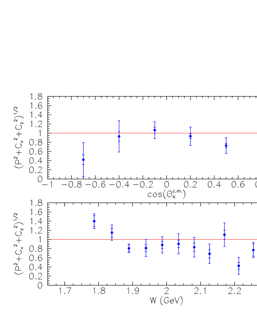
Figure 3: Magnitude of the polarization of the $\Sigma^{0}$ hyperon when averaging over all measured energies and given as a function of angle (top), and alternatively when averaged over all angles given as a function of c.m. energy (bottom). The magnitude, $R_{\Sigma^{0}}$, is not statistically consistent with unity. The error bars are discussed in the text.

3 The Model Hypothesis

The problem at hand is to deduce why the $\Lambda$ polarization in the reaction $\gamma p\to K^{+}\Lambda$, with fully circularly polarized photons is “100%”. This is not a feature of any of at least six highly-developed theoretical models that have been compared with these experimental results, as shown and discussed in Ref. bradford .

Our ansatz is that the reaction proceeds via the creation of a virtual $\overline{s}s$ quark pair in a ${}^{3}S_{1}$ state. A virtual $\phi$ meson is created, in a vector dominance picture, that carries the polarization of the incoming photon, as illustrated in Fig. 4. Alternatively, the $\overline{s}s$ pair is created as part of a complex interaction in the gluon field of the nucleon. Either way, the key assumption is that the $s$ quark is produced in a pure spin state. Next we demand that this polarized quark survives the hadronization process into the final state $\Lambda$ in the form of a pure spin state. We further assume that the $\Lambda$ spin polarization is a faithful representation of that of the $s$ quark contained within it. One can then ask what form the interaction Hamiltonian may take, such that the quark spin is not changed in magnitude but only in its orientation. A possible answer is given by the theory of two-component spinor dynamics merz .

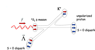
Figure 4: Quark-line cartoon to illustrate one possible scenario in this hypothesis. An $\overline{s}s$ quark pair produced from the photon hadronizes such that the $s$ quark in the $\Lambda$ retains its full polarization after being “precessed” by a spin-orbit interaction, while the $\overline{s}$ quark ends up in the spinless kaon.

In keeping with the ansatz, we construe the interaction to be between a spin $\frac{1}{2}$ quark in the field of a nucleon. The nucleon also has spin $\frac{1}{2}$, but it is unpolarized, so we will for this discussion pretend that it is effectively spinless. Consider the initial quark spin state $\chi_{0}$ to be a linear superposition of eigenstates with respect to the beam ($\hat{z}$) axis taken as positive and negative helicity states $\alpha$ and $\beta$. A fully polarized quark has helicity +1 and is in state $\alpha$.

The interaction Hamiltonian we will consider (because it has the desired property) is that of a spin-orbit interaction between the quark spin and the orbital angular momentum, $\vec{L}$, of the quark with respect to the hardronizing nucleon system:

$$H=\frac{\vec{p}^{2}}{2m}+V(r)+W(r)\vec{L}\cdot\vec{\sigma}$$ (13)

where $V(r)$ is the spin-independent central potential, $W(r)$ is the spin-dependent potential, and $\vec{\sigma}$ are the Pauli spin matrices that act upon $\chi_{0}$. A spin-orbit interaction of the form given in Eq. 13 arises from, for example, a magnetic dipole (of the quark) interaction with an induced magnetic field (due to the quark moving in the electric field of the nucleon). $H$ is a scalar invariant under rotations and reflections, which is the key property needed to obtain the desired result. A rotationally invariant $H$ commutes with $\vec{J}=\vec{L}+\vec{S}$. An incoming state of given helicity, $\alpha$ or $\beta$, is in an eigenstate of $J_{z}=\pm\frac{1}{2}\hbar$, and the scattering state must have with same $J_{z}$. Reflection through any plane must also leave the scattering state unaltered. The scattering matrix, $S$, that acts on $\chi_{0}$, after also considering these requirements of rotational and reflection symmetry, has the form

$$S=\left(\begin{array}[]{cc}g(\theta)&h(\theta)e^{-i\phi}\\ -h(\theta)e^{i\phi}&g(\theta)\end{array}\right)$$ (14)

where $g(\theta)$ is a complex non-spin-flip amplitude, $h(\theta)$ is a complex spin-flip amplitude, and $\phi$ is the azimuthal scattering angle. That is, $h(\theta)$ turns $\beta$ into $\alpha$, with some phase factor, while $g(\theta)$ leaves $\alpha$ as $\alpha$ modified by a phase. The polar angular dependence on the production angle, $\theta$, can only be determined by actually solving the scattering equation. Using Euler’s formula and the Pauli matrices, this is equivalent to

$$S=g(\theta)1+ih(\theta)\hat{n}\cdot\vec{\sigma}$$ (15)

where $\hat{n}=(\vec{\gamma}\times\hat{K}^{+})/|\vec{\gamma}\times\hat{K}^{+}|$ is normal to the scattering plane. Having only two complex amplitudes is not accurate, since the nucleon actually has spin $\frac{1}{2}$ as well, leading to four complex amplitudes for pseudo-scalar meson photoproduction. We proceed anyway, since the proton spin is not polarized and the categorization into spin-flipping and non-flipping amplitudes for the quark itself retains some generality.

The final spin state of the quark, $\chi_{f}$, is given by $S\chi_{0}$. The polarization $\vec{P}_{f}$ of the final spin state is given by the expectation value of $\vec{\sigma}$, with suitable normalization in the denominator of the final-state spin vector:

$$\vec{P}_{f}=<\vec{\sigma}>=\frac{\chi_{f}^{\dagger}\vec{\sigma}\chi_{f}}{\chi_{f}^{\dagger}\chi_{f}}=\frac{\chi_{0}^{\dagger}S^{\dagger}\vec{\sigma}S\chi_{0}}{\chi_{0}^{\dagger}S^{\dagger}S\chi_{0}}$$ (16)

To evaluate this expression we use the density matrix formulation of the initial and final spin states as the way to capture all the phase information in the computation. We use $\rho_{0}=\chi_{0}\chi_{0}^{\dagger}=\frac{1}{2}(1+\vec{P}_{0}\cdot\vec{\sigma})$ and $\rho_{f}=\chi_{f}\chi_{f}^{\dagger}=\frac{1}{2}(1+\vec{P}_{f}\cdot\vec{\sigma})$ and the fundamental formula for evaluating expectations values of an operator $\vec{A}$, that is, $<\vec{A}>=Tr(\rho\vec{A})$. The final state polarization becomes

$$\vec{P}_{f}=\frac{Tr(\rho_{0}S^{\dagger}\vec{\sigma}S)}{Tr(\rho_{0}S^{\dagger}S)}$$ (17)

The denominator in this expression is the differential cross section $d\sigma/d\Omega$. Substituting the expressions for $S$ and $\rho_{0}$, and bringing to bear the necessary trace identities reduces this to

$$\vec{P}_{f}(g^{*}g+h^{*}h+i(g^{*}h-h^{*}g)(\vec{P}_{0}\cdot\hat{n})$$ (18)

$$= (i(g^{*}h-h^{*}g)+2h^{*}h\vec{P}_{0}\cdot\hat{n})\hat{n}+$$

$$(g^{*}g-h^{*}h)\vec{P}_{0}+(g^{*}h+h^{*}g)(\vec{P}_{0}\times\hat{n})$$

For the problem at hand the initial quark polarization is along the beam line, the $\hat{z}$ direction, and can be written $\vec{P}_{0}=(0,0,P_{\odot})$. Now the three terms in Eq. 18 are orthogonal and can be identified with the $\hat{y}$, $\hat{z}$, and $-\hat{x}$ directions. Note the sign reversal on $\hat{x}$ to be consistent with our coordinate system choices in Fig. 1.

We thus have four observables for determining the four real parameters of the two complex amplitudes $g(\theta)$ and $h(\theta)$.

$$\frac{d\sigma}{d\Omega}= g^{*}g+h^{*}h$$ (19)

$$P_{fx}= \frac{g^{*}h+h^{*}g}{g^{*}g+h^{*}h}P_{\odot} \equiv-C_{x}P_{\odot}$$ (20)

$$P_{fy}= i\frac{g^{*}h-h^{*}g}{g^{*}g+h^{*}h} \equiv P$$ (21)

$$P_{fz}= \frac{g^{*}g-h^{*}h}{g^{*}g+h^{*}h}P_{\odot} \equiv C_{z}P_{\odot}$$ (22)

It is easy to check from these equations, having started with a rotationally symmetric spin-orbit Hamiltonian and written it in terms of two amplitudes, that the magnitude of the polarization vector is given by $|\vec{R}|=1$ for any $g(\theta)$ and $h(\theta)$ when $P_{\odot}=1$. That is, a spin-orbit type of interaction preserves the magnitude of the polarization and only rotates it in some fashion. No constraints are placed on the forms of $g(\theta)$ and $h(\theta)$.

The components of the amplitudes can be determined from the experimental results directly. If we write $g=g_{r}e^{i\phi_{g}}$ and $h=h_{r}e^{i\phi_{h}}$ then we find

$$g_{r} = \left(\textstyle\frac{1}{2}\frac{d\sigma}{d\Omega}(1+C_{z})\right)^{1/2},$$ (23)

$$h_{r} = \left(\textstyle\frac{1}{2}\frac{d\sigma}{d\Omega}(1-C_{z})\right)^{1/2},$$ (24)

$$\Delta\phi = \tan^{-1}\frac{P}{C_{x}},$$ (25)

where $\Delta\phi=\phi_{g}-\phi_{h}$ is the phase difference between $g$ and $h$. The overall phase is unimportant.

Preservation of the polarization magnitude is a general property of interactions of the form Eq. 13, as can also be derived by investigating merz the time dependence of a polarization vector $\vec{P}(t)$. By writing the time-dependent Schrödinger equation for $\chi_{0}$ and evaluating the time dependence of the expectation value of $\vec{\sigma}$ one is led to

$$2\hbar\frac{d\vec{P}}{dt}=\vec{L}\times\vec{P}.$$ (26)

This means that the change in the polarization vector is perpendicular to the vector itself, so that $\vec{P}$ “precesses” around $\vec{L}$ in the manner of a magnetic moment precessing around a static magnetic field.

The second puzzle in the experimental results was the observation that $C_{z}\simeq C_{x}+1$. From Eqs. 20 and  22, this observation has the consequence that

$$h^{*}h=\textstyle\frac{1}{2}(g^{*}h+h^{*}g).$$ (27)

Again using the polar representation, this expression shows a simple relationship between the magnitudes of the spin-flip amplitude $h(\theta)$ and the non spin-flip amplitude $g(\theta)$:

$$h_{r}=g_{r}\cos\Delta\phi,$$ (28)

where the phase difference $\Delta\phi$ could be a function of $W$ and $\theta$. It is shown in Ref. bradford that $C_{z}$ it is large and positive in most regions of energy and angle. This means the non spin-flip amplitude $g$ is dominant and the spin-flip amplitude $h$ is small in most regions of energy and angle. Therefore $\cos\Delta\phi$ is a fairly small number and the phase difference $|\Delta\phi|$ is near $\pi/2$.

Thus, the second puzzle would find its explanation in a phenomenology wherein the two interfering amplitudes in this process, spin-flip and non spin-flip, are everywhere proportional to the cosine of their phase difference. The accuracy of this statement hinges on an experimental result that is only of modest precision, as discussed above, and underlines the desirability to make further experimental checks of this interpretation.

4 Discussion and Conclusion

We note that this general picture of the reaction process diverges from the notion that the photon first produces a non-strange $N^{*}$ or $\Delta$ baryon, and that this baryon then couples to the $K^{+}\Lambda$ final state. The latter approach does not build in the idea that the spin of the created strange quark is intimately tied to the spin of the incoming photon. In the standard picture, the spin couplings are treated at the hadronic level, not the quark level. The model hypothesis discussed here was developed largely to account for such a connection.

This model hypothesis can make some testable predictions since there are other observables that have not been measured but ought to have behavior explained in this picture. An example is the case when the photons are linearly polarized and the hyperon recoil polarization is again measured. In that case there are the observables $O_{x}$ and $O_{z}$. The picture suggested here would predict the initial creation of a transversely polarized $s$ quark as part of a ${}^{3}S_{1}$ pair, followed by again a spin-orbit like quark-baryon hadronization interaction that preserves the polarization magnitude. The induced polarization $P$ would again be the third orthogonal component, leading to the prediction

$$O_{x}^{2}+O_{z}^{2}+P^{2}=1$$ (29)

There are a large number of similar predictions which could be examined in the light of this hypothesis.

In summary, this paper has presented some details of recent first-time measurements of the beam-recoil spin-transfer measurements for $K^{+}Y$ photoproduction on the proton. Two puzzles that were raised in a recent talk/paper were discussed. First, why is the net polarization of the $\Lambda$ hyperon in the $K^{+}\Lambda$ final state essentially $100\%$? Second, why is the transferred spin polarization in the $\hat{z}$ direction, $C_{z}$, one unit larger than the in-plane transferred polarization in the $\hat{x}$ direction, $C_{x}$? A model explanation was presented that is built on the idea that the created $s$ quark carries the photon polarization as a pure spin state, and that this quark experiences a spin-orbit type of interaction during hadronization that allows it to “precess” while preserving its magnitude. This was shown explicitly in a model wherein the spin interaction for the quark is categorized into spin flip and non spin-flip amplitudes during hadronization. It was further shown that the ratio of the amplitude magnitudes is given, at all energies and angles, by the cosine of their phase difference; the consequences of this relationship remain to be discovered. While this model hypothesis is somewhat heuristic, especially ignoring the initial proton’s spin, it may nevertheless serve as a starting point for deeper considerations of this problem.

References

- (1) R. Bradford, R. A. Schumacher et al. (CLAS Collaboration), submitted to Phys. Rev. C, arXiv:nucl-ex/0611034.
- (2) P. Ambrozewicz, D. S. Carman, R. J. Feuerbach, M. D. Mestayer, B. A. Raue, R. A. Schumacher , A. Tkabladze et al. (CLAS Collaboration), submitted to Phys. Rev. C, arXiv:hep-ex/0611036.
- (3) J. W. C. McNabb, R. A. Schumacher, L. Todor (CLAS Collaboration), et al., Phys. Rev. C 69, 042201(R) (2004).
- (4) I. S. Barker, A. Donnachie, and J. K. Storrow, Nucl. Phys. B95, 347 (1975).
- (5) R. Bradford, R.A. Schumacher, J. W. C. McNabb, L. Todor, et al. (CLAS Collaboration), Phys. Rev. C 73 035202 (2006).
- (6) This discussion uses the notation and general arguments found in Eugen Merzbacher, Quantum Mechanics, 2nd Ed. (John Wiley and Sons, New York, 1970) pp. 277-293.