First Measurement of Beam-Recoil Observables $C_{x}$ and $C_{z}$ in Hyperon Photoproduction.

Abstract

Spin transfer from circularly polarized real photons to recoiling hyperons has been measured for the reactions $\vec{\gamma}+p\to K^{+}+\vec{\Lambda}$ and $\vec{\gamma}+p\to K^{+}+\vec{\Sigma}^{0}$. The data were obtained using the CLAS detector at Jefferson Lab for center-of-mass energies $W$ between 1.6 and 2.53 GeV, and for $-0.85<\cos\theta_{K^{+}}^{c.m.}<+0.95$. For the $\Lambda$, the polarization transfer coefficient along the photon momentum axis, $C_{z}$, was found to be near unity for a wide range of energy and kaon production angles. The associated transverse polarization coefficient, $C_{x}$, is smaller than $C_{z}$ by a roughly constant difference of unity. Most significantly, the total $\Lambda$ polarization vector, including the induced polarization $P$, has magnitude consistent with unity at all measured energies and production angles when the beam is fully polarized. For the $\Sigma^{0}$ this simple phenomenology does not hold. All existing hadrodynamic models are in poor agreement with these results.

I INTRODUCTION

Photoproduction of strangeness off the proton leading to $K\Lambda$ and $K\Sigma$ states is a fundamental process that is part of the broader field of elementary pseudoscalar meson production. It has been used primarily as a tool to investigate the formation and decay of non-strange baryon resonances in a manner complimentary to $\pi$ and $\eta$ meson production. Spin observables such as those reported here are expected to be sensitive tests of baryon resonance structure and reaction models.

When the photon beam is unpolarized, parity conservation in electromagnetic production allows induced polarization, $P$, of the hyperon only along the axis perpendicular to the reaction plane $\hat{\gamma}\times\hat{K}$. However, when the incoming photons are circularly polarized, that is, when the photons are spin polarized parallel or anti-parallel to the beam direction, giving them net helicity, then this polarization may be transferred in whole or in part to the spin orientation of the produced hyperons within the reaction plane. $C_{x}$ and $C_{z}$ characterize the polarization transfer from a circularly polarized incident photon beam to a recoiling hyperon along orthogonal axes in the reaction plane. This paper reports first measurements of the two double polarization observables, $C_{x}$ and $C_{z}$, for $K^{+}\Lambda$ and $K^{+}\Sigma^{0}$ photoproduction.

Recent measurements of the photoproduction differential cross sections have been published by groups working at Jefferson Lab bradforddsdo , Bonn bonn2 , and SPring-8 leps . Induced hyperon recoil polarizations, $P$, have also been published by Jefferson Lab mcnabb , Bonn bonn2 , and GRAAL graal . The beam linear polarization asymmetry, $\Sigma$, was measured at SPring-8 zegers . These results were obtained with large-acceptance detectors that allowed statistically precise measurements across a broad range of kinematics. Very sparse data exist on the target asymmetry, $T$, from Bonn althoff . A preliminary version of the results reported in this paper was previously given at the NStar 2005 conference nstar .

Much of the recent experimental effort has been motivated by theoretical calculations which suggest that strangeness photoproduction might be a fertile place to search for non-strange baryon resonances that couple strongly to $K^{+}Y$ cap . Quark model states “missing” in the analysis of single pion final states of electromagnetic and hadronic production may merely be “hidden” due to unfavorable coupling strengths or complex multi-pion final states. The less well studied strangeness production channels (as well as other mesonic final states) cast a different light on the baryon resonance spectrum.

The recently published differential cross sections have been tests for a number of single channel theoretical models maid ; mart ; jan ; jan_a ; saghai1 ; ireland ; corthals . These models were mostly tree-level calculations that attempted to extract information about states decaying to $K^{+}\Lambda$ or $K^{+}\Sigma^{0}$ by varying the prescription for the inclusion of baryon resonances, the methods of enforcing gauge invariance, and the introduction of hadronic form factors, etc. As the models were adjusted to the new differential cross section measurements, there was a claim for evidence of a specific new baryonic state maid visible via $K^{+}\Lambda$ production. However, it is clear that there is no unique solution for the baryon resonance content of the differential and single polarization observable data that is currently available penner ; jan ; saghai1 . Since the single channel models failed to produce conclusive results for the baryon resonance content of hyperon photoproduction, let alone undiscovered states, measurements of new observables are needed in order to achieve better understanding from $K^{+}\Lambda$ and $K^{+}\Sigma^{0}$.

Some more recent models have become more sophisticated by moving beyond single channel analyses. These fall into categories of either coupled channel approaches chiang ; shklyar ; saghai2 or of fitting to multiple but independent reaction channels at once  sarantsev ; anisovich ; anisovich2 . On the side of greater simplicity, one can compare the present results with a pure Regge model lag1 ; lag2 that contains no baryon resonance contributions at all. These models will be discussed and compared to the present results later in this paper, however none of the models will have been adjusted to fit the results presented here.

This paper will describe what $C_{x}$ and $C_{z}$ are and how they are measured in Section II. The experimental setup will be outlined in Section III, and specifics of the data analysis will be covered in Section IV. The results of the present measurements and discussion of what was found will be given in Section V, including comparison to predictions of seven different models. Our conclusions will be restated in Section VI.

II FORMALISM AND MEASUREMENT METHOD

Real photoproduction of pseudoscalar mesons is fully described by four complex amplitudes. The bilinear combinations of these amplitudes define 16 observables barker ; knoechlein , summarized in Table 1. Of these sixteen observables, besides the unpolarized differential cross section, there are three single polarization observables and twelve double polarization observables. The single polarization observables include the hyperon recoil polarization ($P$), and the beam $(\Sigma)$ and target $(T)$ polarization asymmetries. The double polarization observables characterize reactions under various combinations of beam, target, and baryon recoil polarization. To uniquely determine the underlying complex amplitudes, one has to measure the unpolarized cross section, the three single polarization observables, and at least four double polarization observables barker ; tabakin1 . To date, only $P$ and $\Sigma$ have been measured extensively and analyzed in models of $K^{+}\Lambda$ and $K^{+}\Sigma^{0}$ photoproduction.

	Required Polarization
Observable	Beam	Target	Hyperon
Single Polarization & Cross Section
A, $\frac{d\sigma}{d\Omega}$	-	-	-
$\Sigma$	linear	-	-
$T$	-	transverse	-
$P$	-	-	along $y^{\prime}$
Beam and Target Polarization
$G$	linear	along $z$	-
$H$	linear	along $x$	-
$E$	circular	along $z$	-
$F$	circular	along $x$	-
Beam and Recoil Baryon Polarization
$O_{x^{\prime}}$	linear	-	along $x^{\prime}$
$O_{z^{\prime}}$	linear	-	along $z^{\prime}$
$C_{x^{\prime}}$	circular	-	along $x^{\prime}$
$C_{z^{\prime}}$	circular	-	along $z^{\prime}$
Target and Recoil Baryon Polarization
$T_{x^{\prime}}$	-	along $x$	along $x^{\prime}$
$T_{z^{\prime}}$	-	along $x$	along $z^{\prime}$
$L_{x^{\prime}}$	-	along $z$	along $x^{\prime}$
$L_{z^{\prime}}$	-	along $z$	along $z^{\prime}$

Table 1: Groupings of all observables for pseudoscalar meson photoproduction. The axis convention used in this paper to define alternate to the “primed” variables $C_{x^{\prime}}$ and $C_{z^{\prime}}$ are discussed in the text. The table is adapted from Ref. barker .

The present measurements were made with a circularly polarized photon beam. Let $P_{\odot}$ represent the degree of beam polarization between $-1.0$ and $+1.0$. The spin-dependent cross section for $K^{+}Y$ photoproduction can be expressed as

$$\rho_{Y}\frac{d\sigma}{d\Omega_{K^{+}}}=\left.{\frac{d\sigma}{d\Omega_{K^{+}}}}\right|_{unpol.}\!\!\!\!\!\!\!\!\!\!\!\left\{1+\sigma_{y}P+P_{\odot}(C_{x}\sigma_{x}+C_{z}\sigma_{z})\right\}.$$ (1)

Here $\rho_{Y}$ is twice the density matrix of the ensemble of recoiling hyperons $Y$ and is written

$$\rho_{Y}=(1+\vec{\sigma}\cdot\vec{P}_{Y}),$$ (2)

where $\vec{\sigma}$ are the Pauli spin matrices and $\vec{P}_{Y}$ is the measured polarization of the recoiling hyperons. In Eq. 1 the spin observables are the induced polarization $P$, and the polarization transfer coefficients $C_{x}$ and $C_{z}$. For further discussion a definite coordinate system is needed.

Figure 1 illustrates the coordinate system used in this paper. In the literature there are two conventions for discussing the beam-recoil observables. The polarization of the hyperons in the production plane can be described with respect to a $z$ axis chosen along the incident beam direction (i.e. the helicity axis of the photons) or along the momentum axis of the produced $K^{+}$. Because a polarization vector transforms as a vector in three-space, this choice is of no fundamental significance. In this paper we select the $z$ axis along the photon helicity direction because it will be seen that the transferred hyperon polarization is dominantly along $\hat{z}$ defined in Fig. 1. Model calculations for $C_{x}$ and $C_{z}$ supplied to us in the $\{\hat{x}^{\prime},\hat{z}^{\prime}\}$ basis were rotated about the $\hat{y}$-axis to the $\{\hat{x},\hat{z}\}$ basis.

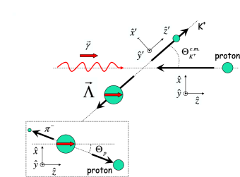
Figure 1: (Color online) In the overall reaction center of mass, the coordinate system can be oriented along the outgoing $K^{+}$ meson $\{\hat{x}^{\prime},\hat{y}^{\prime},\hat{z}^{\prime}\}$ or along the incident photon direction $\{\hat{x},\hat{y},\hat{z}\}$. The dotted box represents the rest frame of the hyperon, and the coordinate system used for specifying the polarization components. The red arrows represent polarization vectors.

With the axis convention chosen to give the results their simplest interpretation, we correspondingly define our $C_{x}$ and $C_{z}$ with signs opposite to the version of Eq. 1 given in Ref. barker . This will make $C_{z}$ positive when the $\hat{z}$ and $\hat{z}^{\prime}$ axes coincide at the forward meson production angle, meaning that positive photon helicity results in positive hyperon polarization along $\hat{z}$.

The connection between the measured hyperon recoil polarization $\vec{P}_{Y}$ and the spin correlation observables $P$, $C_{x}$, and $C_{z}$, is obtained by taking the expectation value of the spin operator $\vec{\sigma}$ with the density matrix $\rho_{Y}$ via the trace: $\vec{P}_{Y}=Tr(\rho_{Y}\vec{\sigma})$. This leads to the identifications

$$P_{Yx} = P_{\odot}C_{x}$$ (3)

$$P_{Yy} = P$$ (4)

$$P_{Yz} = P_{\odot}C_{z}.$$ (5)

Thus, the transverse or induced polarization of the hyperon, $P_{Yy}$, is equivalent to the observable $P$, while the $\hat{x}$ and $\hat{z}$ components of the hyperon polarization in the reaction plane are proportional to $C_{x}$ and $C_{z}$ via the beam polarization factor $P_{\odot}$. Physically, $C_{x}$ and $C_{z}$ measure the transfer of circular polarization, or helicity, of the incident photon on an unpolarized target to the produced hyperon.

II.1 Hyperon Decay and Beam Helicity Asymmetries

Hyperon polarizations $\vec{P}_{Y}$ are measured through the decay angular distributions of the hyperons’ decay products. The decay $\Lambda\to\pi^{-}p$ has a parity-violating weak decay angular distribution in the $\Lambda$ rest frame. The decay of the $\Sigma^{0}$ always proceeds first via an $M1$ radiative decay to a $\Lambda$. In either case, $\vec{P}_{Y}$ is measured using the angular distribution of the decay protons in the hyperon rest frame. In the specified coordinate system $i\in\{x,y,z\}$ is one of the three axes. The decay distribution, $I_{i}(\cos\theta_{i})$, is given by

$$I_{i}(\cos\theta_{i})={\textstyle\frac{1}{2}}(1+\nu\alpha P_{Yi}\cos\theta_{i}),$$ (6)

where $\theta_{i}$ is the proton polar angle with respect to the given axis in the hyperon rest frame. The weak decay asymmetry, $\alpha$, is taken to be $0.642$. The factor $\nu$ is a “dilution” arising in the $\Sigma^{0}$ case due to its radiative decay to a $\Lambda$, and which is equal to $-1/3$ in the $\Lambda$ rest frame. A complication arose for us because we measured the proton angular distribution in the rest frame of the parent $\Sigma^{0}$. This led to a value of $\nu=-1/3.90$, as discussed in Appendix A. For the $K^{+}\Lambda$ analysis $\nu=+1.0$. Extraction of $P_{Yi}$ follows from fitting the linear relationship of $I_{i}(\cos\theta_{i})$ vs. $\cos\theta_{i}$.

The components of the measured hyperon polarization, $\vec{P}_{Y}$, are then related to the polarization observables using the relations in Eqs. 3, 4, and 5. The crucial experimental aspect is that when the beam helicity is reversed ($P_{\odot}\to-P_{\odot}$), so are the in-plane components of the hyperon polarization.

In each bin of kaon angle $\cos\theta_{K^{+}}^{c.m.}$, total system energy $W$, and proton angle $\cos\theta_{i}$, let $N_{\pm}$ events be detected for a positive (negative) beam helicity according to

$$N_{\pm}(\cos\theta_{i})=\epsilon_{K}\epsilon_{p}Q_{\pm}\left[SI_{i}(\cos\theta_{i})+N_{BG}\right].$$ (7)

$Q_{\pm}$ represents the number of photons with net helicity $\pm P_{\odot}$ incident on the target. $S$ designates all cross section and target related factors for producing events in the given kinematic bin. The spectrometer has a bin-dependent kaon acceptance defined as $\epsilon_{K}$. The protons from hyperon decay distributed according to Eq. 6 are detected in bins, usually 10 in number, that each have an associated spectrometer acceptance defined as $\epsilon_{p}$. In fact, $\epsilon_{K}$ and $\epsilon_{p}$ are correlated since the reaction kinematics connect the places in the detector these particles will appear. This correlation is a function of $W$, $\cos\theta_{K^{+}}^{c.m.}$, and $\cos\theta_{i}$, but is assumed to be beam helicity independent. We denote the correlated acceptance as $\epsilon_{K}\epsilon_{p}$. The method used here avoids explicitly computing this correlation. The term $N_{BG}$ designates events due to “backgrounds” from other physics reactions or from event misidentifications. The hyperon yield-fitting procedure discussed in Sec. IV.2 removes $N_{BG}$, and the associated residual uncertainty is discussed in Sec. IV.4.

If the beam helicity, $P_{\odot}$, can be “flipped” quickly and often, then by far the most straightforward way to obtain the $C_{i}$ values is to construct the ensuing asymmetry, $A$, as a function of proton angle. In each proton angle bin we record the number of events, $N_{\pm}$, in each beam helicity state and compute the corresponding asymmetry as:

$$A(\cos\theta_{i})=\frac{N_{+}-N_{-}}{N_{+}+N_{-}}=\alpha\nu P_{\odot}C_{i}\cos\theta_{i}.$$ (8)

In this ratio the correlated detector acceptances and various systematic effects cancel. An exception would be if there were a change in the track reconstruction efficiency due to a difference in the beam intensity between the two beam polarization states. Estimates of such phenomena proved negligibly small on the scale of the results presented later. If the beam intensity in the two beam polarization states were not equal there would be a measured beam intensity asymmetry (BIA) given by

$$A_{BIA}=\frac{Q_{+}-Q_{-}}{Q_{+}+Q_{-}}.$$ (9)

This quantity is angle independent and therefore does not influence the value of the slope of $A(\cos\theta_{i})$.

II.2 Frame Transformation

The hyperon polarizations were evaluated in the hyperon rest frames according to the discussion in the previous sub-section. The overall center of mass (c.m.) frame of the reaction is reached by a boost along the $\hat{z^{\prime}}$ axis, and we need to understand if and how the polarization of the hyperons is changed in this transformation. When boosting a baryon’s spin projections from one frame to another, one must take into account the Wigner-Thomas precession that arises from the non-commutativity of rotations and boosts. In an initial frame $S$, suppose a particle has velocity $\vec{\beta}$ $(=\vec{p}c/E)$ with respect to the boost direction at a polar angle $\theta$. In an arbitrary boosted frame $\tilde{S}$, let the transformed velocity be described by $\tilde{\vec{\beta}}$ with respect to the boost direction at a polar angle $\tilde{\theta}$. Let the corresponding boost parameters be $\Gamma$ for the frame boost, $\gamma$ for the particle in the $S$ frame and $\tilde{\gamma}$ in the boosted $\tilde{S}$ frame, where $\gamma=1/\sqrt{1-\beta^{2}}$. It can be shown giebink  wignernote that for an arbitrary boost in the $\{\hat{x},\hat{z}\}$ plane the Wigner-Thomas precession angle, $\alpha_{W}$, about the $\hat{y}$ axis is given by

$$\sin\alpha_{W}=\frac{1+\Gamma}{\gamma+\tilde{\gamma}}\sin(\theta-\tilde{\theta}).$$ (10)

This relativistic rotation of the polarization direction is important, for example, when transforming the laboratory-measured $(S)$ proton recoil polarization in the reaction $p(\vec{e},e^{\prime}\vec{p})\pi^{0}$ to the center of mass frame of the virtual photon and target nucleon $(\tilde{S})$ wijesooriya  schmieden . In this example the boost direction is generally not collinear with the nucleon momentum in $S$ or $\tilde{S}$, and the Wigner-Thomas precession angle can become large.

In the present measurement, the boost to be performed is from the hyperon rest frame $(S)$ to the c.m. frame of the real photon and nucleon $(\tilde{S})$. Implicit in this discussion is that the polarization is described in both frames with respect to the same coordinate system. The boost is along the hyperon momentum direction, so both $\theta$ and $\tilde{\theta}$ are zero. Therefore the spin precession angle $\alpha_{W}$ is identically zero for all hyperon production angles. The center-of-mass value for the hyperon polarization is thus the same as it is in the hyperon rest frame. We must measure $\vec{P}_{Y}$ in the hyperon rest frame, but it is the same in the overall reaction c.m. frame.

III EXPERIMENTAL SETUP

The data analyzed to measure $C_{x}$ and $C_{z}$ were recorded by the CLAS spectrometer in Hall B at Jefferson Lab. Data were produced at two different electron energies, $E_{elec}=2.4$ and $2.9$ GeV. The 2.4 GeV data set was previously analyzed in combination with a third data set at 3.1 GeV to extract differential cross sections bradforddsdo and for $\Lambda$ and $\Sigma^{0}$ recoil polarizations mcnabb . These present measurements are the first reported results from the 2.9 GeV data set. All data sets were recorded under the same (“g1c”) run conditions. In the previous papers, the beam polarization and measurement of the in-plane recoil polarization were not relevant, but now we discuss these points.

The incident polarized electron beam was used to create a secondary beam of circularly polarized photons using the Hall B photon tagging system. Bremsstrahlung photons were produced by colliding the longitudinally polarized electron beam with a gold foil radiator. The residual momenta of the recoiling electrons were measured with a hodoscope behind a dipole magnetic field. This information was used to determine the energy and predict the arrival time of photons striking the physics target. The energy range of the tagging system spanned from 20% to 95% of the endpoint energy. The rate of tagged photons was about $1.4\times 10^{7}$/sec. Detailed information about the CLAS photon tagging system is given in tagger . The physics target consisted of a 18 cm long cell of liquid hydrogen located at the center of the CLAS detector.

The CLAS detector is a multi-particle large acceptance spectrometer that incorporates a number of subsystems. The start counter (SC), a scintillator counter surrounding the target, was used to obtain a fast timing signal as particles left the target. The tracking system of the detector included 34 layers of drift chamber cells. A toroidal magnetic field provided by a superconducting magnetic bent the trajectories of charged particles through the tracking volume for momentum determination. For this experiment, the magnetic field was operated so that positively charged particles were bent outward, away from the beamline. Finally, as particles left the detector, an outer scintillator layer, the time-of-flight (or TOF) array made a final timing measurement. The readout trigger required coincidence between timing signals from the photon tagger, SC, and the TOF. More general information about the detector and its performance can be obtained from Ref. clas0 ; the detector configuration at the time of this experiment is further detailed in Refs.mcnabbthesis ; bradfordthesis .

III.1 Beam Polarization

Extraction of $C_{x}$ and $C_{z}$ from the beam helicity asymmetry, as discussed in Section IV, required accurate knowledge of the photon beam polarization. Since Hall B has no Compton polarimeter to directly measure the photon beam polarization, this information was obtained through a two step process. The polarization of the incident electron beam was measured with a Møller polarimeter, and a well-known formula then gave the polarization of the secondary photon beam.

The Hall B Møller polarimeter moeller is a dual-arm coincidence device which exploits the helicity dependence of Møller scattering to measure the polarization of the incident electron beam. Beam electrons were scattered elastically from electrons in the polarimeter target. A pair of quadrupole magnets collected the scattered electrons on a pair of scintillation counters. Helicity-dependent yields, $N_{+}$ and $N_{-}$, were recorded. From these yields, the electron beam polarization was measured according to

$$A_{elec}=\frac{N_{+}-N_{-}}{N_{+}+N_{-}}=A_{z}P_{elec}P_{T},$$ (11)

where $A_{elec}$ is the helicity-dependent asymmetry, $A_{z}$ is the analyzing power of the polarimeter iron foil target, $P_{T}$ is the polarization of the target material, and $P_{elec}$ is the polarization of the incident beam.

Operation of the Møller polarimeter disrupted the beam and was periodically done separately from the main data taking. The various measurements were averaged for each run period and reported as a single polarization. The results are shown in Table 2. The uncertainties shown are estimated random and averaging uncertainties. The estimated systematic uncertainty on the Møller measurements was $\pm 3\%$ moeller . The values of $P_{elec}$ are typical of the Jefferson Lab electron beam when using a strained GaAs cathode and laser to produce electrons.

Beam Energy	$e^{-}$ Beam Polarization
2.4 GeV	$0.654\pm 0.015$
2.9 GeV	$0.641\pm 0.012$

Table 2: Electron beam polarizations, $P_{elec}$, used in these measurements.

The polarization of the beam was flipped at the injector to the accelerator at a rate of 30 Hz in a simple non-random $+-+-$… sequence. The beam helicity state was recorded event by event in the data stream.

The energy-dependent circular polarization, $P_{\odot}(E_{\gamma})$, of the photons originating from the bremsstrahlung of the longitudinally polarized electrons on a radiator was computed using the expression

$$P_{\odot}(E_{\gamma})=\frac{y(4-y)}{4-4y+3y^{2}}P_{elec},$$ (12)

where $y=E_{\gamma}/E_{elec}$ is the fraction of photon energy $E_{\gamma}$ to beam energy $E_{elec}$, and $P_{elec}$ is the polarization of the electron beam. This expression is a slightly rewritten version of Eq. 8.11 in Ref. maximon . The photon polarization is maximal at the bremsstrahlung endpoint and falls rather slowly with decreasing photon energy. Over the photon energy range used in this measurement we had $0.440<P_{\odot}/P_{elec}<0.995$.

IV DATA ANALYSIS

IV.1 Particle Identification and Event Selection

Particle identification for this analysis was identical to that reported for our differential cross section analysis bradforddsdo . In general, particle identification was based on time-of-flight. For each track of momentum $\vec{p}$, we compared the measured time-of-flight, $TOF_{m}$, to a hadron’s expected time-of-flight, $TOF_{h}$, for a kaon, pion, or proton of identical momentum. Cuts were placed on the difference between the measured and expected time-of-flight, $\Delta TOF=TOF_{m}-TOF_{h}$.

Because our measurement technique relied on the self-analyzing nature of the hyperon recoil polarizations, we selected events exclusively involving the charged final state of the decaying hyperons according to $\Lambda\to p\pi^{-}$ and $\Sigma^{0}\to\gamma\Lambda\to\gamma p\pi^{-}$. Three criteria were used to select such events. First, all events were required to have both a $K^{+}$ and a proton track. Second, events were required to have a $p\left(\gamma,K^{+}\right)Y$ missing mass consistent with the mass of a $\Lambda$ or $\Sigma^{0}$ hyperon. Finally, we did not require explicit detection of the $\pi^{-}$ from the hyperon decays, but we required that the $p\left(\gamma,K^{+}p\right)\pi^{-}\left(\gamma\right)$ missing mass be consistent with a $\pi^{-}$ (or $\gamma\pi^{-}$ for $K^{+}\Sigma^{0}$ events). While CLAS was able to detect some of the $\pi^{-}$ tracks directly, acceptance losses reduced the event statistics excessively. To further increase the acceptance of events, we relaxed the fiducial cuts employed in the cross section analysis to permit more tracks near the detector edges. This increased the yield of useful events by a factor of about 60%. Specific cuts to select each hyperon species were developed and are detailed in Ref. bradfordthesis .

IV.2 Binning and Yield Extraction

Hyperon yields were divided into kinematic bins in photon energy ($E_{\gamma}$), recoiling kaon angle in the c.m. frame $(\cos\theta_{K}^{c.m.})$, the angle of the decay proton in the hyperon rest frame $(\cos\theta_{i})$, and the helicity of the incident photon beam. Bin widths and limits are detailed in Table 3.

	$E_{\gamma}$ (GeV)			$\cos\theta_{K^{+}}^{c.m.}$			$\cos\theta_{i}$
Channel	Low	High	$\Delta$	Low	High	$\Delta$	Low	High	$\Delta$
$K^{+}\Lambda$	0.9375	2.7375	0.1	-0.85	0.95	0.2	-1.0	1.0	0.2
$K^{+}\Sigma^{0}$	1.1375	2.7375	0.1	-0.85	0.95	0.3	-1.0	1.0	0.4

Table 3: Binning for $C_{x}$ and $C_{z}$. $K^{+}\Lambda$ observables used a total of 3420 bins, while the $K^{+}\Sigma^{0}$ observables had 1020 bins. The “low” and “high” of each kinematic variable in the table are the edges of our kinematic coverage, not the bin centers. The $\Delta$ columns give the width of the bins.

Two independent hyperon yield extractions were performed in each bin. The first extraction employed a fit to the $p\left(\gamma,K^{+}\right)Y$ missing mass spectrum in the region of the $\Lambda$ and $\Sigma^{0}$ mass peaks (1.0 to 1.3 GeV/c²). Hyperon peaks were each fit to a Gaussian line shape, while the backgrounds were modeled with a polynomial of up to second order. Since the background shape varied slowly across the kinematic coverage, the background shape employed in the fits was selected on a bin-by-bin basis; see Ref. bradforddsdo for sample yield fits. The second extraction method relied on side-band subtraction in which the background was assumed to be smooth under the hyperons.

IV.3 Asymmetry Calculation and Slope Extraction

Within each $\{E_{\gamma}$ , $\cos\theta_{K^{+}}^{c.m.}$, $\cos\theta_{i}\}$ bin, the helicity dependent yields were used to calculate the beam-helicity asymmetry according to the sum of Eqs. 8 and  9. Two different versions of this asymmetry were calculated. The fit-based asymmetry method, or FBA, was largely based on yields determined by the Gaussian-plus-background fits, with the side-band yields used in bins where the fits failed. The second calculation employed only sideband-subtracted asymmetries, or SBA; all fits were turned off for this calculation.

The asymmetries were computed vs. $\cos\theta_{i}$, and linear fits were used to extract the slopes of the distributions. The free parameters were the product $\alpha\nu P_{\odot}C_{i}$ and $A_{BIA}$ in Eq 9. Some sample distributions are shown in Figs. 2 and 3 for the $\Lambda$ and $\Sigma^{0}$ cases, respectively. In general, the asymmetry distributions were very well fit with a sloped line. Counting statistics were poorest at lower photon energies and backward kaon angles, where the cross sections were smallest and the kaon decay probability was largest, but the statistics improved rapidly for mid- to forward-going kaons and higher photon energies. Results with and without constraining $A_{BIA}$ to be zero were in very good agreement, but we did not constrain this offset to be zero to avoid bias from this source. The average fitted value was $A_{BIA}=0.002$ with a standard deviation of 0.027.

The overall fit quality is well summarized by the distribution of $\chi^{2}$ per degree-of-freedom. Figure 4 shows this distribution for the linear fits used in the measurement of $C_{z}$ for the $K^{+}\Lambda$ case. This figure shows that the actual $\chi^{2}$ distribution is consistent with the expected distribution, indicated by the smooth curve superimposed on the histogram. The actual and expected $\chi^{2}$ distributions were consistent for all results reported in this paper.

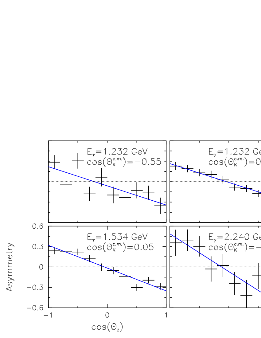
Figure 2: (Color online) Representative hyperon yield asymmetries as a function of proton decay angle for the case of the $C_{z}$ observable for the $\Lambda$. The scales are the same in all plots.

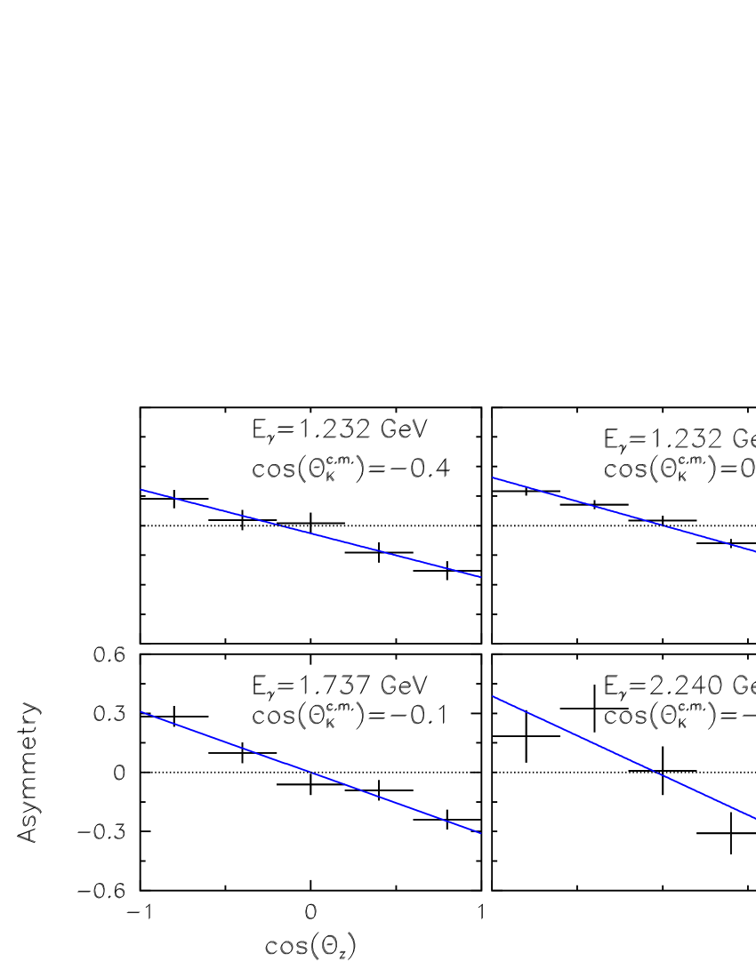
Figure 3: (Color online) Representative hyperon yield asymmetries as a function of proton decay angle for the case of the $C_{z}$ observable for the $\Sigma^{0}$. The scales are the same in all plots.

Figure 4: (Color online) Distribution of the reduced $\chi^{2}$ values for fits with 8 degrees of freedom for the $C_{z}$ fits in the $K^{+}\Lambda$ case.

Within each $\{E_{\gamma}$, $\cos\theta_{K^{+}}^{c.m.}\}$ kinematic bin, we compared the FBA and SBA asymmetries, as shown in Fig. 5. In the large majority of kinematic bins, the distributions were statistically consistent, though in a few bins the two methods differed significantly. The final results were based on the asymmetry calculation (FBA or SBA) that was fit best by the straight line. The differences were used to estimate the systematic uncertainty associated with the yield extraction.

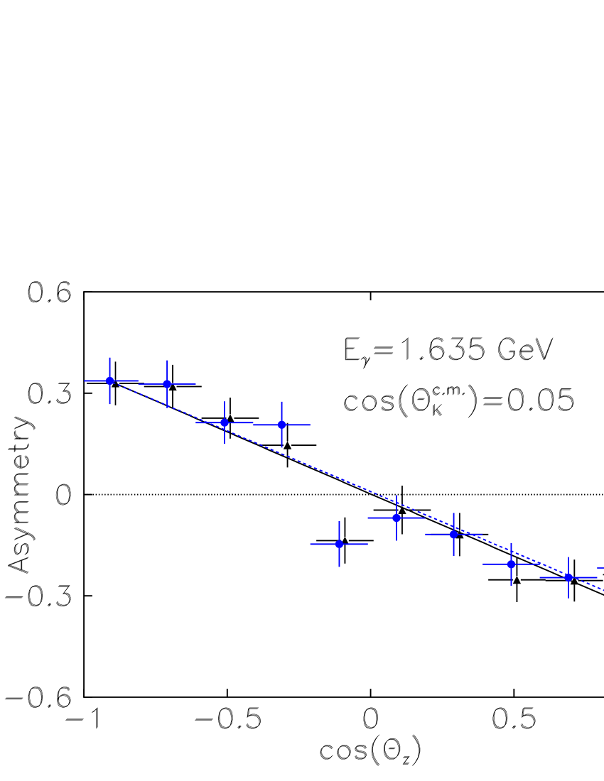
Figure 5: (Color online) Hyperon yield asymmetries as a function of proton decay angle. The two sets of points were obtained via the FBA (black triangles) and SBA (blue circles) methods, respectively. The two fitted lines, which are proportional to $C_{z}$ for the $K^{+}\Lambda$ case, show a visible difference, as discussed in the text.

IV.4 Systematic Uncertainties

As shown in Eq. 8, four factors are key to measurements of $C_{x}$ and $C_{z}$: (1) the beam helicity asymmetry, (2) the beam polarization, (3) the weak decay asymmetry parameter, and (4) the dilution factor. Uncertainties on each one of these factors may contribute to systematic uncertainty in our results.

We studied dependence of the beam helicity asymmetry on the yield extraction method. As discussed in Section IV.3, we performed two different yield extractions and we calculated two versions of the beam helicity asymmetry, the fit-based asymmetry (FBA) and the side-band subtracted asymmetry (SBA). Within each $\{E_{\gamma}$, $\cos\theta_{K}^{c.m.}\}$ kinematic bin, we fit each asymmetry distribution independently and measured the difference between the extracted slopes. This slope difference was interpreted as a point-to-point systematic error due to the yield extraction method. This slope difference was added in quadrature with the error on the extracted slope and propagated through the analysis. The good agreement between the methods was the basis for our treating $N_{BG}$ in Eq. 7 as negligible. Uncertainties in this paper, then, include statistical errors plus the estimated point-by-point systematic error due to the yield extraction.

The CLAS Møller polarimeter has uncertainties in the analyzing power of the reaction and in the polarimeter’s target polarization moeller , which resulted in a systematic uncertainty of $\pm 0.016$ on the final observables. Measurements from the polarimeter also had their own statistical uncertainties, shown in Table 2, which also contributed to the global systematic error. When propagated, the contribution to the systematic error is $\pm 0.022$.

The $\Lambda$ weak decay asymmetry parameter $\alpha$ has a well-documented uncertainty pdg06 of $\pm 0.013$. The contribution to the global systematic uncertainty is then $\pm 0.020$. The dilution factor $\nu$, discussed in Appendix A, is a purely computational quantity that is assumed to have negligible uncertainty compared to the other sources discussed here.

Our analysis method for $C_{x}$ and $C_{z}$ should result in a vanishing measured transverse polarization of the hyperons, $P_{Yy}$. That is, the helicity asymmetry of the out-of-plane projection of the hyperons’ polarization, as defined in Fig. 1, must be zero. This test formed a useful systematic check of our method. To measure “$C_{y}$”, the same analysis procedure was applied as for $C_{x}$ and $C_{z}$, the only difference being that the proton direction was projected onto $\hat{y}$ in the hyperon rest frame. The results were consistent with zero over a large range of kinematics, but $C_{y}$ was statistically nonzero for fairly forward kaon c.m. angles for both hyperons. This was attributed to the measurement $\hat{y}=\hat{\gamma}\times\hat{K}$ being less accurate at very forward kaon laboratory angles due to detector geometry and resolution effects. Such distortions would similarly affect $C_{x}$, for example by letting a large $P_{Yz}$ mix into small values of $P_{Yx}$. As a result, there is an angle-dependent systematic uncertainty of $\pm 0.08$ for $\Lambda$ observables at $\cos\theta_{K^{+}}^{c.m.}>0.55$, and $\pm 0.17$ for $\Sigma^{0}$ observables at $\cos\theta_{K^{+}}^{c.m.}>0.35$.

When summed in quadrature, we estimate a total global systematic uncertainty for the $K^{+}\Lambda$ results as $\pm 0.03$ for $\cos\theta^{c.m.}_{K^{+}}<0.55$ and $\pm 0.09$ for $\cos\theta^{c.m.}_{K^{+}}>0.55$. We estimate a total global systematic uncertainty for the $K^{+}\Sigma^{0}$ results as $\pm 0.03$ for $\cos\theta^{c.m.}_{K^{+}}<0.35$ and $\pm 0.17$ for $\cos\theta^{c.m.}_{K^{+}}>0.35$. The systematic uncertainty in $W$ was $\pm 2$ MeV at the bin centers.

V RESULTS

V.1 $C_{x}$ and $C_{z}$ Results for $K^{+}\Lambda$

As discussed in Section II, the transfer of circular polarization from the incident photon beam to the recoiling hyperons leads to the observable $C_{z}$ along the beam direction and $C_{x}$ in the $\hat{\gamma}\times\hat{K}$ reaction plane and perpendicular to the beam axis. The results for the $W$ dependence for the reaction $\vec{\gamma}+p\to K^{+}+\vec{\Lambda}$ are given in Figs. 6 and 7. The same results are presented as a function of kaon c.m. angle in Figs. 8 and 9. The given error bars combine the statistical uncertainties and the estimated point-to-point systematic uncertainties arising from the fits to the helicity asymmetries.

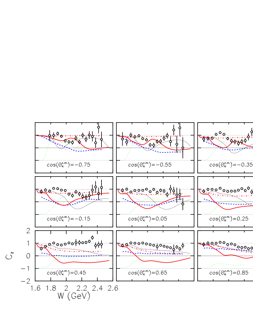
Figure 6: (Color online) The observable $C_{z}$ for the reaction $\vec{\gamma}+p\to K^{+}+\vec{\Lambda}$, plotted as a function of the c.m. energy $W$. The circles are the results of this measurement, with uncertainties discussed in the text. The thin dashed (green) curves are from Kaon-MAID maid , the thick solid (red) curves are from SAP saghai2 , the thick dashed (blue) curves are from BG sarantsev2 , the thin solid (black) curves are from RPR corthals , and the thick dot-dashed (magenta) curves are from GENT jan . The thick dot-dashed (red) curves are from GLV lag1 ; lag2 . The thin dotted (blue) curves are from SLM shklyar .

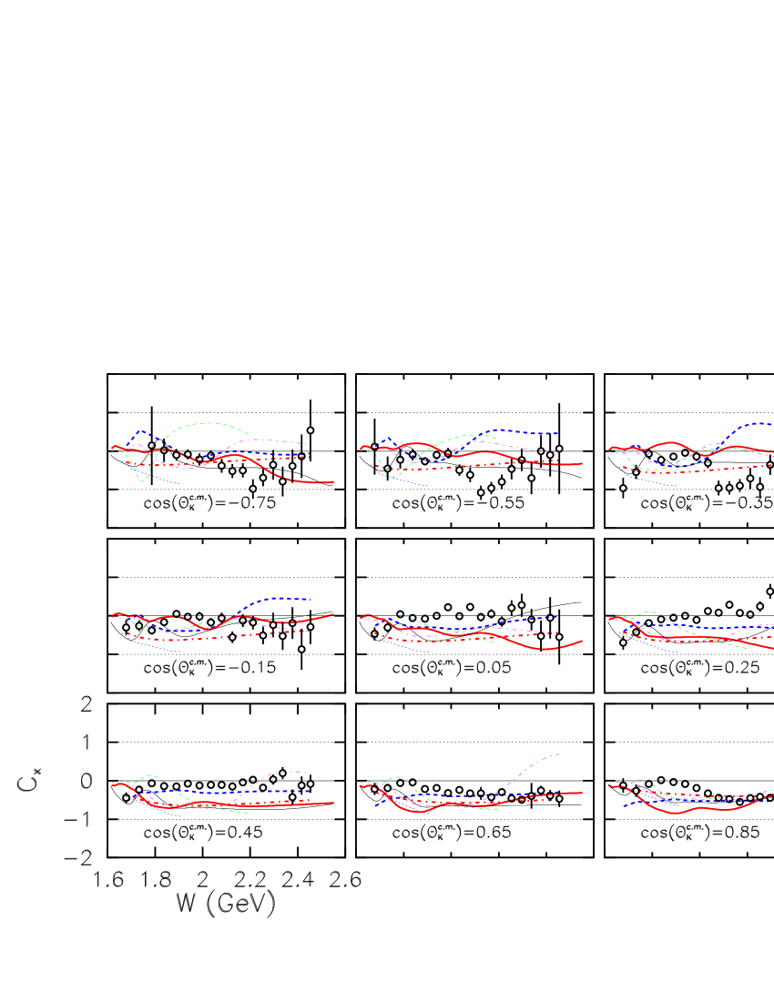
Figure 7: (Color online) The observable $C_{x}$ for the reaction $\vec{\gamma}+p\to K^{+}+\vec{\Lambda}$, plotted as a function of the c.m. energy $W$. The circles are the results of this measurement, with uncertainties discussed in the text. The thin dashed (green) curves are from Kaon-MAID maid , the thick solid (red) curves are from SAP saghai2 , the thick dashed (blue) curves are from BG sarantsev2 , the thin solid (black) curves are from RPR corthals , and the thick dot-dashed (magenta) curves are from GENT jan . The thick dot-dashed (red) curves are from GLV lag1 ; lag2 . The thin dotted (blue) curves are from SLM shklyar .

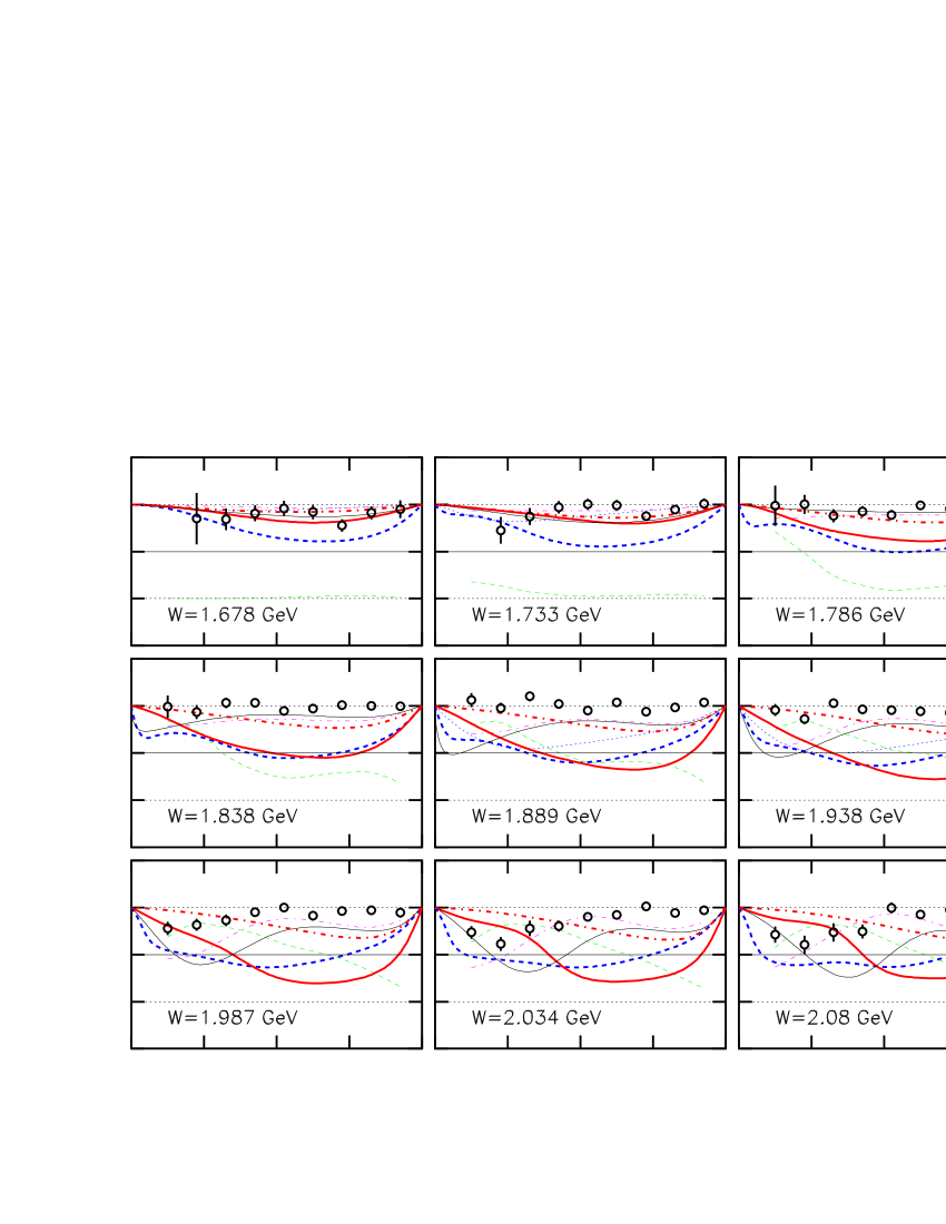
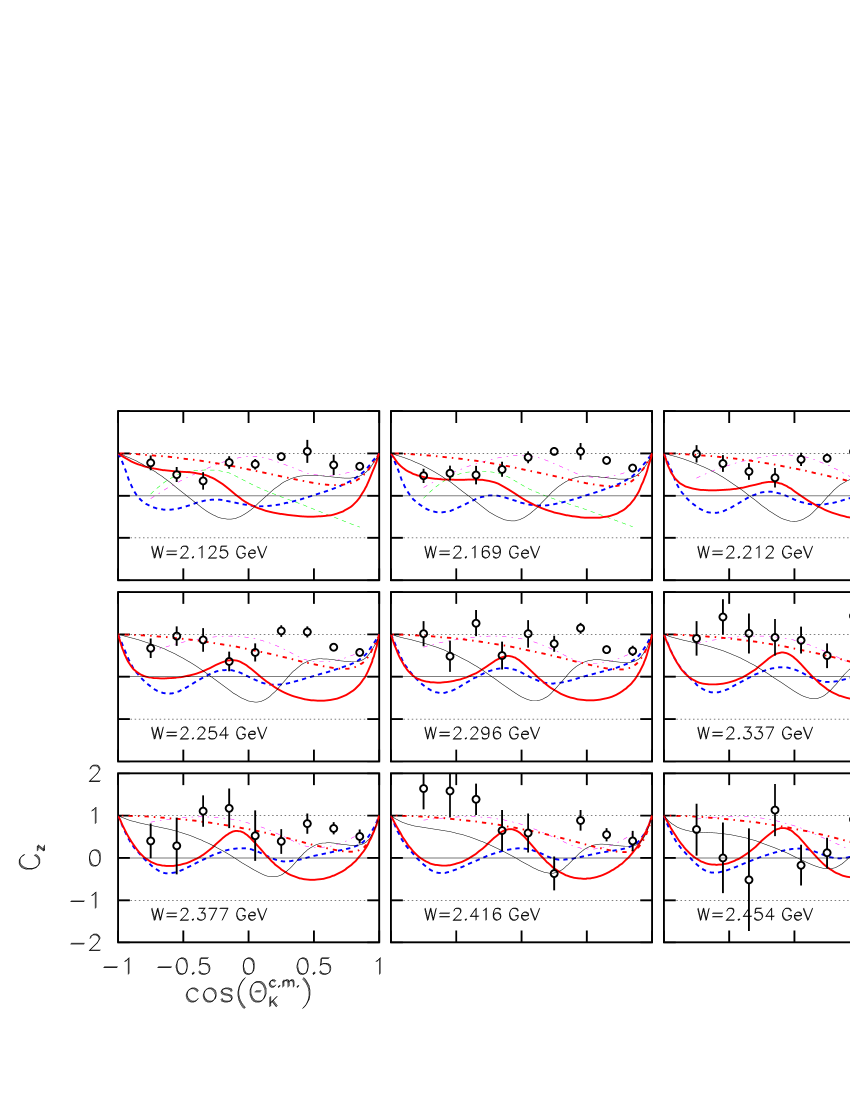
Figure 8: (Color online) The observable $C_{z}$ for the reaction $\vec{\gamma}+p\to K^{+}+\vec{\Lambda}$, plotted as a function of the kaon angle. The 18 panels are for increasing values of $W$ in steps of about 50 MeV. The circles are the results of this measurement, with uncertainties discussed in the text. The thin dashed (green) curves are from Kaon-MAID maid , the thick solid (red) curves are from SAP saghai2 , the thick dashed (blue) curves are from BG sarantsev2 , the thin solid (black) curves are from RPR corthals , and the thick dot-dashed (magenta) curves are from GENT jan . The thick dot-dashed (red) curves are from GLV lag1 ; lag2 . The thin dotted (blue) curves are from SLM shklyar .

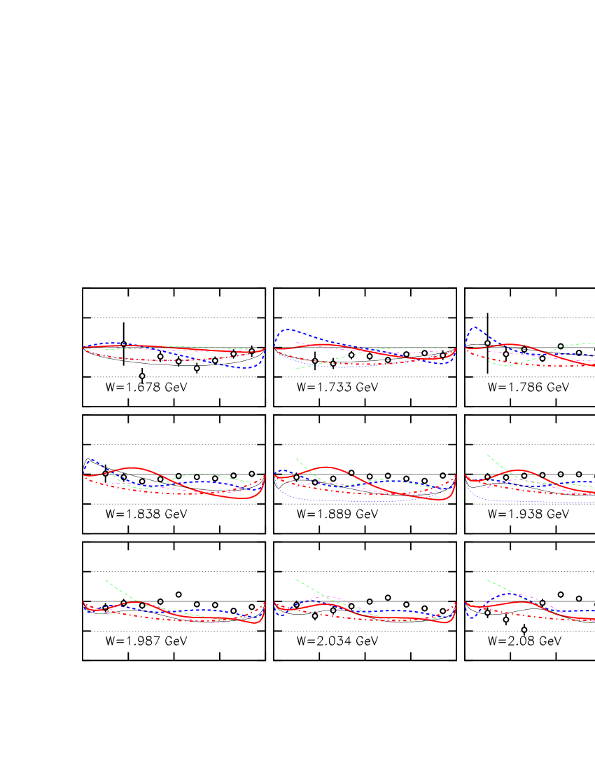
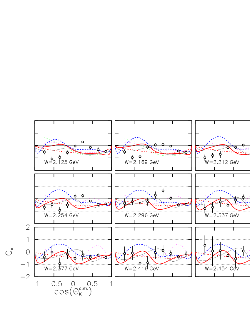
Figure 9: (Color online) The observable $C_{x}$ for the reaction $\vec{\gamma}+p\to K^{+}+\vec{\Lambda}$, plotted as a function of the kaon angle. The 18 panels are for increasing values of $W$ in steps of about 50 MeV. The circles are the results of this measurement, with uncertainties discussed in the text. The thin dashed (green) curves are from Kaon-MAID maid , the thick solid (red) curves are from SAP saghai2 , the thick dashed (blue) curves are from BG sarantsev2 , the thin solid (black) curves are from RPR corthals , and the thick dot-dashed (magenta) curves are from GENT jan . The thick dot-dashed (red) curves are from GLV lag1 ; lag2 . The thin dotted (blue) curves are from SLM shklyar .

It is immediately evident in these results that, qualitatively, the photon polarization is largely transferred to the $\Lambda$ hyperon along the $\hat{z}$ direction in the c.m. frame. Figure  8 shows that from threshold up to about 1.9 GeV the $\Lambda$ data exhibit $C_{z}\sim+1$, which means it has nearly the full polarization transferred to it, irrespective of the production angle of the kaon. For higher values of $W$ one can see fall-offs of the value of $C_{z}$ as a function of kaon c.m. angle. However, for kaons produced in the forward hemisphere, the nearly full transfer effect is present up to about 2.1 GeV, as seen in Fig. 6. Above this energy the forward-angle value of $C_{z}$ decreases with increasing $W$. The concomitant values of $C_{x}$ are generally closer to zero, as seen in Fig. 7, with significant excursions to negative values for a combination of backward kaon angle and high energies, and again for the very forward angles and higher energies.

This striking observation of large and quasi-constant values of $C_{z}$ is why we chose to present our results in the $\{x,z\}$ coordinate system rather than the $\{x^{\prime},z^{\prime}\}$ system. It can be interpreted in terms of a picture wherein the photon excites an $s$-channel resonance which decays with no orbital angular momentum, $L$, along the $\hat{z}$ direction. In a simple classical picture of a two-particle $s$-channel interaction, any orbital angular momentum is normal to $\hat{z}$. To conserve the $z$ component of angular momentum, the hyperon must then carry it in the form of spin polarization. In the case of $K^{+}\Lambda$ near threshold, the reaction is thought to be dominated by the $S_{11}$ partial wave, for which this argument applies. There is no reason for this picture to hold up, however, when multiple amplitudes conspire to result in the observed polarization. Thus, it is surprising how “simple” the result for $K^{+}\Lambda$ appears.

At higher energies and backward kaon c.m. angles the “simple” pictures gives way to more interference structure in both $C_{z}$ and $C_{x}$. For example, in Fig. 7, $C_{x}$ takes values close to $-1.0$ for $\cos\theta_{K^{+}}^{c.m.}<-0.35$ and $W>2.1$ GeV. Also at the most forward angles for $W>2.1$ GeV there is a monotonic trend downward in both $C_{z}$ and $C_{x}$.

V.2 Combining $C_{x}$, $C_{z}$ Results with Results for $P$

There are several inequalities that must be satisfied by the observables available in pseudo-scalar meson photoproduction barker ; goldstein ; tabakin1 . Artru, Richard, and Soffer soffer pointed out that for a circularly polarized beam there is a rigorous inequality

$$R^{2}\equiv P^{2}+C_{x}^{2}+C_{z}^{2}\leq 1$$ (13)

among the three polarization observables, where $P$ is the same as the measured $P_{Yy}$, the induced recoil polarization of the baryon. For a $100\%$ circularly polarized photon beam, $\vec{R}$ is equivalent to $\vec{P}_{Y}$ defined in Eq. 2. In this case the relationship says that the magnitude of the three orthogonal polarization components may have any value up to unity. There is no a priori requirement that the hyperon be produced fully polarized except in the extreme forward and backward directions where orbital angular momentum plays no role. Any rotation of the coordinate system about $\hat{y}$ would redefine the $C_{i}$ but leave the inequality unchanged, since the baryon polarization transforms as a 3-vector under spatial rotations.

A significant test of the present results for $C_{x}$ and $C_{z}$ is therefore compatibility with the previously-published mcnabb results for the induced hyperon recoil polarization $P$. (We note that those earlier data have been confirmed up to $E_{\gamma}=1.5$ GeV by measurements at GRAAL graal .) While the helicity asymmetries used in the present measurement are sensitive to $C_{x}$ and $C_{z}$, the $\hat{y}$ helicity asymmetry must be zero by reason of parity conservation. On the other hand, our previous measurement ignored the beam polarization information and was sensitive to $P$ but not $C_{x}$ and $C_{z}$. Taken together, the measurements should obey the constraint given above.

Figure 10 displays the values for $R_{\Lambda}$ for the $\Lambda$ hyperons obtained when combining the present results with those of McNabb et al. mcnabb . The binning is the same as for Figs. 8 and 9, with the upper limit of $W=2.29$ GeV set by the range of the previously-published data for $P$. For ease of comparison we include the previously-published data for $P$ in Fig. 11. The data in Fig. 10 combine the present $C_{x}$ and $C_{z}$ results with $P$ values interpolated to closely match the present $W$ and kaon angle bins. The error bars are given by standard error propagation, approximating the uncertainties on $C_{x}$ and $C_{z}$ as statistically independent.

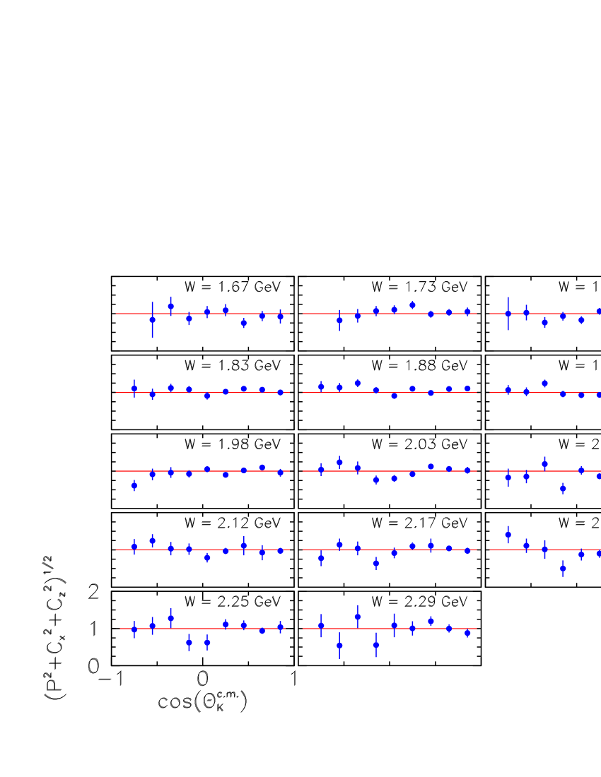
Figure 10: (Color online) The magnitude of the $\Lambda$ hyperon polarization observable vector $R_{\Lambda}=\sqrt{P^{2}+C_{x}^{2}+C_{z}^{2}}$ in the same binning as Figs. 8 and  9. $R_{\Lambda}$ is consistent with unity over all values of $W$ and kaon angle.

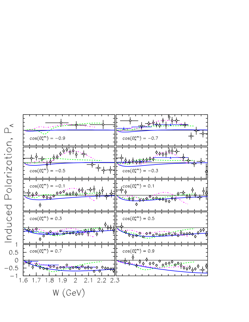
Figure 11: (Color online) Induced recoil polarization, $P$, of the $\Lambda$ hyperon in $\gamma+p\to K^{+}+\vec{\Lambda}$. Open circles (black) from Ref. mcnabb , triangles (blue) from Ref. bonn2 . The dashed (green) curves are from Kaon-MAID maid , the dot-dashed (magenta) curves are from GENT jan , and the solid (blue) curves are the Regge model GLV lag1 ; lag2 .

It is striking how close the magnitude of $R_{\Lambda}$ is to its maximum possible value of +1 across all values of $W$ and kaon angle. Taking the weighted mean over the data at all energies and angles we find

$$\overline{R}_{\Lambda}=1.01\pm 0.01.$$ (14)

This is consistent with unity within the given statistical uncertainty on the mean, and certainly within our stated systematic uncertainty on the beam polarization. Some data points exceed the maximum allowed value of unity by several sigma, but this must be expected on statistical grounds. The $\chi^{2}$ for a fit to the hypothesis that $R_{\Lambda}=1$ is 145 for 123 degrees of freedom, for a reduced chi-square of 1.18, which is a good fit. Thus, the deviations are probably dominated by random measurement errors.

One may therefore conclude that the $\Lambda$ hyperons produced in $\vec{\gamma}+p\to K^{+}+\vec{\Lambda}$ with circularly polarized photons appear 100% spin polarized. Since this situation is not required by the kinematics of the reaction, there must be some as yet unknown dynamical origin of this phenomenon.

The $\Lambda$ polarization direction is determined largely by the photon helicity direction, since generally $C_{z}$ is the largest component. Careful examination of Figs. 6 and 11 shows where the induced polarization $P$ “fills in” missing strength of $C_{z}$. For example, at forward angles and high energies, $C_{z}$ is reduced from unity, easily seen in the bottom right panel of Fig. 6, but the induced polarization $P$ is large and negative in Fig. 11. As another example, near $W=2.08$ GeV and $\cos\theta_{K^{+}}^{c.m.}=-0.55$, $P$ is large and positive just where $C_{z}$ dips down to about $+0.2$ and $C_{x}$ is at $-0.6$.

V.3 Possible relation between $C_{x}$ and $C_{z}$

Looking at the results shown in Figs. 6 through 9 suggests an empirical relation between $C_{x}$ and $C_{z}$, specifically

$$C_{z}\simeq C_{x}+1.$$ (15)

Taking the weighted mean of $D\equiv C_{z}-C_{x}-1$ over all values of $W$ and kaon angle leads to the value $\overline{D}=0.054\pm 0.012$. In this case the $\chi^{2}$ for a fit to the hypothesis of Eq. 15 is 306 for 159 degrees of freedom, or 1.92 for the reduced $\chi^{2}$. This is a poor fit, so our confidence in the accuracy of this simple empirical relationship is limited, and indicates that it needs experimental confirmation. We can offer no explanation for this curious relationship. Linearity between $C_{x}$ and $C_{z}$ suggests rotating the coordinate axes by $+\pi/4$ about the $\hat{y}$ axis, such that $C_{x}$ and $C_{z}$ are mapped onto two new axes, $C_{1}$ and $C_{2}$. The new variable $C_{2}$ would be approximately constant with a value of $1/\sqrt{2}$ and all the variation with $W$ and kaon angle would be in $C_{1}$. $C_{2}$ would represent a helicity dependent but otherwise constant contribution to the cross section, while $C_{1}$ would contain dynamical information. In that case, the three observables $C_{x},C_{z}$, and $P$ would be reduced to a single independent quantity. One could define a phase angle, $\psi$, between the induced and the transferred polarizations as $\psi=\tan^{-1}P/C_{1}$. The two relationships from Eqs. 13 and 15, together with $\psi$, would specify all three components of the $\Lambda$ polarization. The limited statistical precision of the present results precludes drawing a stronger conclusion here.

V.4 Comparison to Hadronic Models

The results are compared in Figs. 6 through 16 with a group of recent calculations based on published models. It should be noted that none of these calculations were refitted for the purpose of matching these new data. In that sense, the curves shown in these figures are extrapolations of the models to previously unmeasured observables.

First consider some recent effective-Lagrangian models of hyperon photoproduction that evaluate tree-level Feynman diagrams including resonant and non-resonant exchanges of baryons and mesons. The advantages of the tree-level approach, i.e. to not include the effects of channel coupling and rescattering, are to limit complexity and to identify the dominant trends.

For $K^{+}\Lambda$ production, the model of Mart and Bennhold mart has four baryon resonance contributions. Near threshold, the steep rise of the cross section is accounted for with the $N^{*}$ states $S_{11}(1650)$, $P_{11}(1710)$, and $P_{13}(1720)$. To explain the broad cross-section bump in the mass range above these resonances bradforddsdo ; bonn2 , they introduced the $D_{13}(1895)$ resonance that was predicted in the relativized quark models of Capstick and Roberts cap and Löring, Metsch, and Petry loring to have especially strong coupling to the $K^{+}\Lambda$ channel. In addition, the higher mass region has contributions, in this model, from the exchange of vector $K^{*}(892)$ and pseudovector $K_{1}(1270)$ mesons. The hadronic form factors, cutoff masses, and the prescription for enforcing gauge invariance were elements of the model for which specific choices were made. The content of this model is embedded in the Kaon-MAID code maid which was used for the comparisons in this paper. This model was fitted to preliminary results from the experiment at Bonn/SAPHIR bonn1 , and offers a fair description of those results.

Analysis by Saghai et al. saghai1 using the same cross section data showed that, by tuning the background processes involved, the need for the extra resonance was removed. Also, Janssen et al. jan ; jan_a (designated GENT here) showed that the same data set was not complete enough to make firm statements since models with and without the presence of the hypothesized $N^{*}(1895)D_{13}$ resulted in equally good fits to the data. A subsequent related analysis ireland which also fitted to photon beam asymmetry measurements from SPring-8 zegers and electroproduction data measured at Jefferson Lab mohring , indicated weak evidence for one or more of $S_{11}$, $P_{11}$, $P_{13}$, or $D_{13}(1895)$, with the $P_{11}$ solution giving the best fit. The conclusion was that a more comprehensive data set would be required to make further progress.

Recently, more elaborate model calculations have been undertaken that consider amplitude-level channel coupling or at least simultaneous fitting to several incoherent reaction channels. Penner and Mosel penner found fair agreement for the $K^{+}\Lambda$ data without invoking a new $D_{13}$ structure. Chiang et al. chiang showed that coupled channel effects are significant at the $20\%$ level in the total cross sections when including pionic final states. Shklyar, Lenske, and Mosel shklyar (designated SLM here) used a unitary coupled-channel effective Lagrangian model applied to $\pi$ and $\gamma$ -induced reactions to find dominant resonant contributions from $S_{11}(1650)$, $P_{13}(1720)$, and $P_{13}(1895)$ states, but not from $P_{11}(1710)$ or $D_{13}(1895)$. Their conclusion held despite the discrepancies between previous cross section data from CLAS mcnabb and SAPHIR bonn2 .

A dynamical coupled-channel model of $K^{+}\Lambda$ photoproduction which emphasized intermediate $\pi N$ states was presented by Julia-Diaz et al. saghai2 (designated SAP here). The model was constrained by results for the hadronic $\pi N\to KY$ channels. To avoid duality issues, $t$-channel exchange was limited only to non-resonant $K$ exchange. Using published photoproduction bradforddsdo ; bonn2 and hadronic cross section data, and the $\Lambda$ polarization data mcnabb ; zegers ; althoff , they sought the dominant baryon resonance contributions to $K^{+}\Lambda$ photoproduction. The model demonstrated dominant contributions from the $N^{*}$ states $S_{11}(1535)$, $P_{13}(1900)$, and $D_{13}(1520)$. Contributions from three new nucleon resonances were found to be significant, specifically $D_{13}(1954)$, $S_{11}(1806)$, and $P_{13}(1893)$. The model showed significant sensitivity to induced polarization $P$ of the $\Lambda$, so one may expect similar sensitivities in $C_{x}$ and $C_{z}$.

A partial wave analysis of the combined data sets for the reactions $\gamma p\to\pi N,\eta N,K^{+}\Lambda,K^{+}\Sigma^{0},K^{0}\Sigma^{+}$ has been reported by a group from Bonn, Gatchina, and Giessen sarantsev ; anisovich ; anisovich2 (designated BG here). The method used a relativistically invariant operator expansion method with relativistic Breit-Wigner representations of selected resonances and reggeized $t$-channel exchanges. Some close-in-mass resonances were coupled using a K-matrix formalism, but overall unitarity violation was allowed. The analysis included the differential cross sections, beam asymmetry for the $\eta$ and the $\Lambda$ cases, and induced recoil polarizations $P$ for the $\Lambda$ and the $\Sigma^{0}$. We note that the $KY$ CLAS cross section data used in the fits were from Ref. mcnabb , and not the newer and more complete results from Ref. bradforddsdo . Compared to other recent models, BG takes into account a larger range of experimental information simultaneously. The spin observables were found to be vital to extract the signatures of resonances as revealed by their mutual interferences. Strong evidence was found for several new $N^{*}$ states including $P_{11}(1840)$ and $D_{13}(1875)$, with weaker evidence for a $D_{13}(2170)$. It might be expected that “new” resonances that coupled significantly to $KY$ and are seen via their effect on spin observables should also have a significant impact on $C_{x}$ and $C_{z}$.

In another recent approach, Corthals, Ryckebusch, and Van Cauteren corthals used a “Regge plus resonance” (RPR) picture to reproduce the CLAS differential cross sections bradforddsdo , recoil polarizations mcnabb , and LEPS beam asymmetries zegers for $K^{+}\Lambda$ production. By fixing the few parameters of a Regge model of $K^{*}$ and $K$ exchange at energies between 5 and 16 GeV, they found four acceptable ways of describing the available high energy data slac . They evolved these solutions into the nucleon resonance region as a way to describe the “background” to the $K^{+}\Lambda$ baryon resonance production cross section. Despite concerns about breaking duality, the advantage of this approach is the relatively small number of free parameters that are needed when compared to $s$-channel dominated isobar models. The latter generally require evaluation of many more diagrams, even at tree level, to approach the measured cross sections. A standard group of “core” resonances was included, the $S_{11}(1650)$, the $P_{13}(1720)$, and the $P_{11}(1710)$, together with a small set of extra $N^{*}$ resonances. Three acceptable fits to the data were obtained. The set of additional $N^{*}$ resonances tested were a $P_{13}(1900)$, a $P_{11}(1900)$, and a $D_{13}(1900)$. Remarkably, one satisfactory solution required no additional baryon resonances at all. The other solutions showed the need for a $P(1900)$ resonance, but the $D_{13}(1900)$ hypothesis did not lead to better fits. The authors concluded that the experimental information is still not precise enough to make an unambiguous case for the resonance contribution(s) in the 1900 MeV mass range. However, a shortcoming of this RPR approach is that it only works for the forward angle region where the Regge parameterization of the cross section can be expected to work. Much of the sensitivity to resonance contributions that shows up more strongly at mid and back angles is thus ignored. It is of interest, therefore, to see how the extrapolations of these RPR solutions, with no additional fitting, match the observables reported in this paper.

Although it is to be expected that $s$-channel resonance structure is a significant component of the $K^{+}\Lambda$ and $K^{+}\Sigma^{0}$ reaction mechanisms, it is instructive to compare to a model that has no such content at all. The model of Guidal, Laget, and Vanderhaeghen lag1 ; lag2 (GLV) is such a model, in which the exchanges are restricted to two linear Regge trajectories corresponding to the vector $K^{*}$ and the pseudovector $K_{1}$. The model was fit to higher-energy photoproduction data where there is little doubt of the dominance of these exchanges. In this paper, we extend that model into the resonance region in order to make a critical comparison.

Having introduced the recent models of hyperon photoproduction, we proceed with some remarks on their behavior in relation to the present results. The models have in common that at threshold the values are $C_{z}=+1.0$ and $C_{x}=0.0$, which is as expected on the basis of the naive picture introduced above in which there is no orbital angular momentum available to carry off any of the $\hat{z}$ component of angular momentum. The exception is the Kaon-MAID model maid which clearly contains a sign error, since it starts at $C_{z}=-1.0$ at threshold. We chose not to reverse this sign by hand but to show the model curve exactly as it is publicly available. Furthermore, Fig. 8 shows that the BG, SAP, and SLM models correctly show that $C_{z}\to+1.0$ at the extreme scattering angles $\cos\theta_{K^{+}}^{c.m.}\to+1.0$. This must be the case since the $z$ component of angular momentum must be conserved via the hyperon spin in this limit. In the same angle limit $C_{x}\to 0$ and all models exhibit this correctly. For $\cos\theta_{K^{+}}^{c.m.}\to-1.0$ the same limits hold again, and the RPR, BG, and SAP models show this correctly, while GENT appears not to extrapolate to these limits.

The next remark is that none of the existing models can be said to do even a fair job predicting the behavior of $C_{z}$ and $C_{x}$ anywhere away from threshold. Only the older model GENT of Janssen et al. jan ; jan_a approximates the qualitative finding that $C_{z}$ is large and positive over most of the measured range. The follow-on model of RPR corthals is less successful by comparison. It is notable that the pure Regge GLV model lag1 ; lag2 , containing only two trajectories and no parameters adjusted to fit the resonance-region data, does no worse than the much more elaborate hadrodynamic models.

We take the poor agreement of existing reaction models with the results as an indication that all models will be able to use these results to refine their contents.

V.5 Comparison to pQCD Limits

Afanasev, Carlson, and Wahlquist afanasev studied polarized parton distributions via meson photoproduction in a model where pQCD was used to describe direct photoproduction of a meson from a quark. The approach is applicable for high transverse momenta where short-range processes are dominant. It was used in the analysis of the reaction $p(\vec{\gamma},\vec{p})\pi^{0}$ with circularly polarized photons in Ref. wijesooriya . Assuming helicity conservation, this model predicted

$$P=C_{x^{\prime}}=0$$ (16)

and

$$C_{z^{\prime}}=\frac{s^{2}-u^{2}}{s^{2}+u^{2}}$$ (17)

in the $\{x^{\prime},z^{\prime}\}$ basis of Fig. 1, where $s$, $t$, and $u$ are the usual Mandelstam variables. In the limit of massless quarks $C_{z^{\prime}}\to 0$ as $|t|\to 0$, and $C_{z^{\prime}}\to 1$ when $|u|\to 0$ at large angles and large $|t|$. The model further assumes the polarization of the struck quark is the same as the polarization of the outgoing hyperon, undiluted by hadronization effects. In the present discussion of $p(\vec{\gamma},\vec{\Lambda})K^{+}$, the strange quark is expected to carry the $\Lambda$ spin as expected in the quark model. The “short-range process” involves the creation of an $s\overline{s}$ quark pair. The light-cone momentum fraction of the active quark, $x$, is defined afanasev for photoproduction as

$$x=\frac{-t}{s+u}.$$ (18)

In the present measurements we have $0.06<x<0.6$. Thus, we span the regime where the struck quark could be a strange sea quark, which hadronizes into a $\Lambda$ hyperon while the anti-strange quark produces the kaon. But at large $|t|$ where this approach could be valid we are in the valence quark regime.

Since our results show that $C_{z}$ is large and positive over most of our kinematic range, it is clear that quark helicity in the baryon is not conserved in this reaction. Nevertheless one can look at the kinematic range where Eq. 17 is thought to be most applicable. Figure 12 shows our results for the largest $|t|$ values measured, stemming from $\cos\theta_{K^{+}}^{c.m.}=-0.75$, as a function of $t$. In the limit of large kaon angle, helicity conservation requires $C_{z^{\prime}}$ to approach unity with our axis definition. Rotating the prediction to yield $C_{x}$ and $C_{z}$ results in the dashed lines in the figure. The agreement with the model is fair to good at large values of $|t|$. Whether or not this is fortuitous is uncertain, since the domain of applicability of the model is not well defined and non-perturbative effects clearly dominate the data at lower $|t|$.

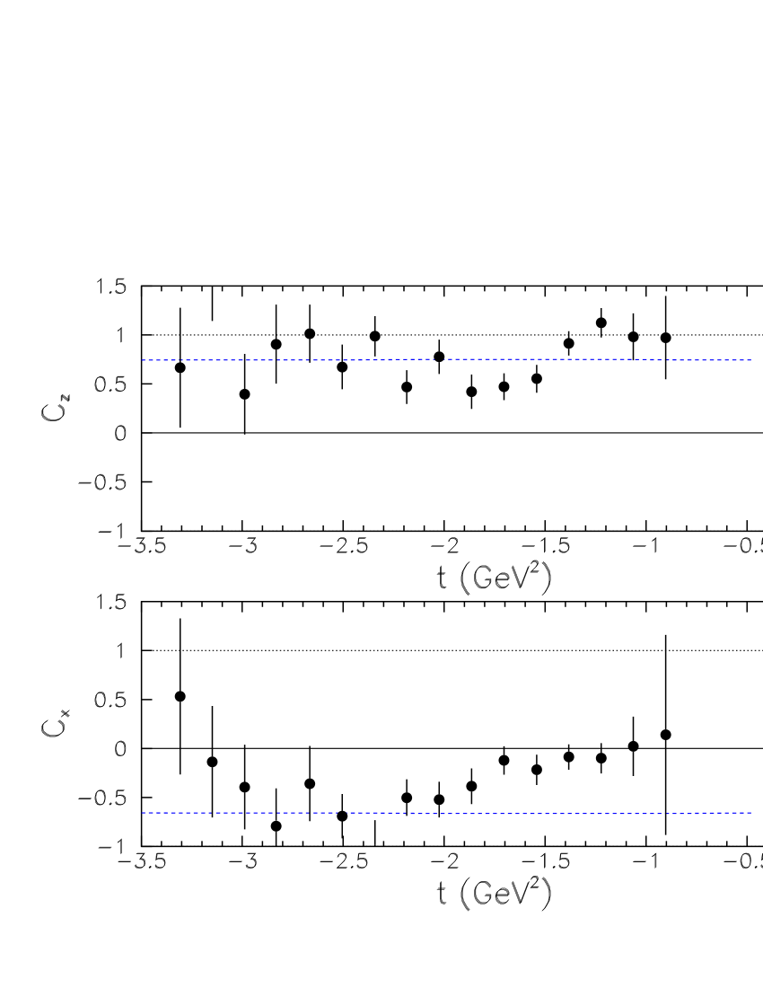
Figure 12: (Color online) The observables $C_{z}$ and $C_{x}$ for the reaction $\vec{\gamma}+p\to K^{+}+\vec{\Lambda}$, plotted as a function of $t$. The dashed (blue) curves are a prediction afanasev ; wijesooriya  from perturbative QCD assuming helicity conservation at the quark level.

Thus, the correct interpretation of this reasonable agreement with the model is not clear. The partial success of this model for the present results on $K^{+}\vec{\Lambda}$ production is in contrast to its complete failure when applied to $\pi^{0}\vec{p}$ photoproduction  wijesooriya in a similar range of $W$. In that measurement the recoiling protons are always much less polarized than the pQCD model suggested.

V.6 Comparison to Electroproduction

The present results for photoproduction can be compared to previous measurements for the reaction $p(e,e^{\prime}K^{+}\Lambda)$ made by CLAS carman . Additional observables arise in electroproduction on account of the extra spin degrees of freedom associated with the virtual photons at finite values of $Q^{2}$. However, the formalism of the electroproduction structure functions merges smoothly into the limiting case of photoproduction at $Q^{2}=0$ (GeV/c)², as written explicitly, for example, in Ref. knoechlein . The electroproduction results were averaged over the range $0.3<Q^{2}<1.5$ (GeV/c)² and also averaged over the azimuthal angle between the electron scattering and the hadronic reaction planes. The transferred polarization component along the direction of the virtual photon, called $P^{\prime}_{z}$ in Ref. carman , is large (between +0.6 and +1.0) and roughly independent of the kaon angle for values of $W$ at 1.69, 1.84, and 2.03 GeV. There is a mild trend toward smaller values of $P^{\prime}_{z}$ with increasing kaon angle. This is consistent with our findings discussed above, where $C_{z}$ is close to +1.0 for the same $W$ values and across all kaon angles, as seen in Fig. 8. In the electroproduction measurement the orthogonal $\hat{x}$ axis was chosen in the electron scattering plane, while in the present paper we can only choose it in the hadronic reaction plane. However, we note that the corresponding $P^{\prime}_{x}$ values in electroproduction are small ($<+0.2$) across all kaon angles and $W$ values. This is again in qualitative agreement with our observed values of $C_{x}$. Thus, we can conclude that the photo- and electro- production measurements show the same qualitative behavior, meaning that there is no rapid departure from the photoproduction systematics as one moves out in $Q^{2}$ from zero to about 1.5 (GeV/c)².

V.7 Results for the $\Sigma^{0}$

In the quark model the ud quarks in the $\Sigma^{0}$ are in a spin triplet state instead of a spin singlet as in the $\Lambda$. The created strange quark is not alone in determining the spin of the overall hyperon in the $\Sigma^{0}$. Thus one may expect the behavior of $C_{x}$ and $C_{z}$ for the $\Sigma^{0}$ to differ from that of the $\Lambda$. Figures 13 to 16 present these results, and indeed it is immediately clear that the trends in this case are not the same as in the previous discussion. Note first that only 6 kaon angle bins were used, centered at $\cos\theta_{K^{+}}^{c.m.}=-0.7$ to $+0.8$ in steps of $0.3$. This was necessitated by the reduced sensitivity to the $\Sigma^{0}$ polarization due to the previously-discussed dilution caused by the $\Sigma^{0}\to\gamma\Lambda$ decay. Despite coarser binning, the statistical precision of the $\Sigma^{0}$ results is still less good than the $\Lambda$ results by a factor of 2 to 3.

The most dramatic differences can be seen comparing the forward-hemisphere values of $C_{z}$ for the $\Sigma^{0}$ in Fig. 13 with the $\Lambda$ in Fig. 6. Near $\cos\theta_{K^{+}}^{c.m.}=+0.45$, $C_{z}$ for the $\Lambda$ is at unity for the whole range in $W$, while for the $\Sigma^{0}$ it falls from $+1.0$ at threshold to large negative values at the highest $W$. The trends of the $C_{x}$ values for the $\Sigma^{0}$ in Fig. 14 are, with limited statistical precision, similar to those of the $\Lambda$ shown in Fig. 7: $C_{x}$ is predominantly negative. The angular distributions for the $\Sigma^{0}$ in Fig. 15 are compared to those for the $\Lambda$ in Fig. 8: the panels are placed to have the same $W$ bins in the same location. At $W=1.889$ GeV, for example, the $\Sigma^{0}$ has a $C_{z}$ of about $+0.5$, while for the $\Lambda$ it is at $+1.0$. At $W=2.296$ GeV the $C_{z}$ for the $\Sigma^{0}$ is about zero, while for the $\Lambda$ it is large and positive. The corresponding values of $C_{x}$ are similar between the two hyperons, as seen in comparing Figs. 16 and 9.

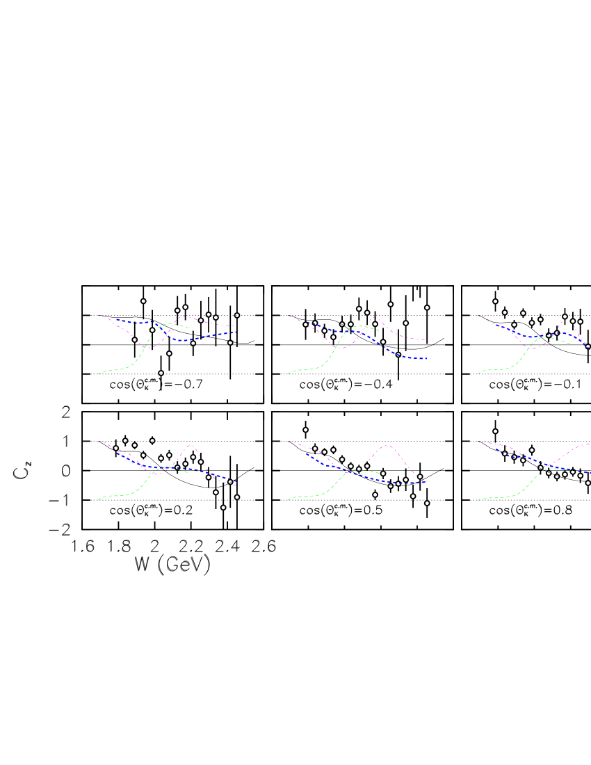
Figure 13: (Color online) The observable $C_{z}$ for the reaction $\vec{\gamma}+p\to K^{+}+\vec{\Sigma}^{0}$, plotted as a function of the c.m. energy $W$. The circles are the results of this measurement, with uncertainties discussed in the text. The thin dashed (green) curves are from Kaon-MAID maid , the thick dashed (blue) curves are from BG sarantsev2 , the thin solid (black) curves are from RPR corthals , and the thick dot-dashed (magenta) curves are from GENT jan .

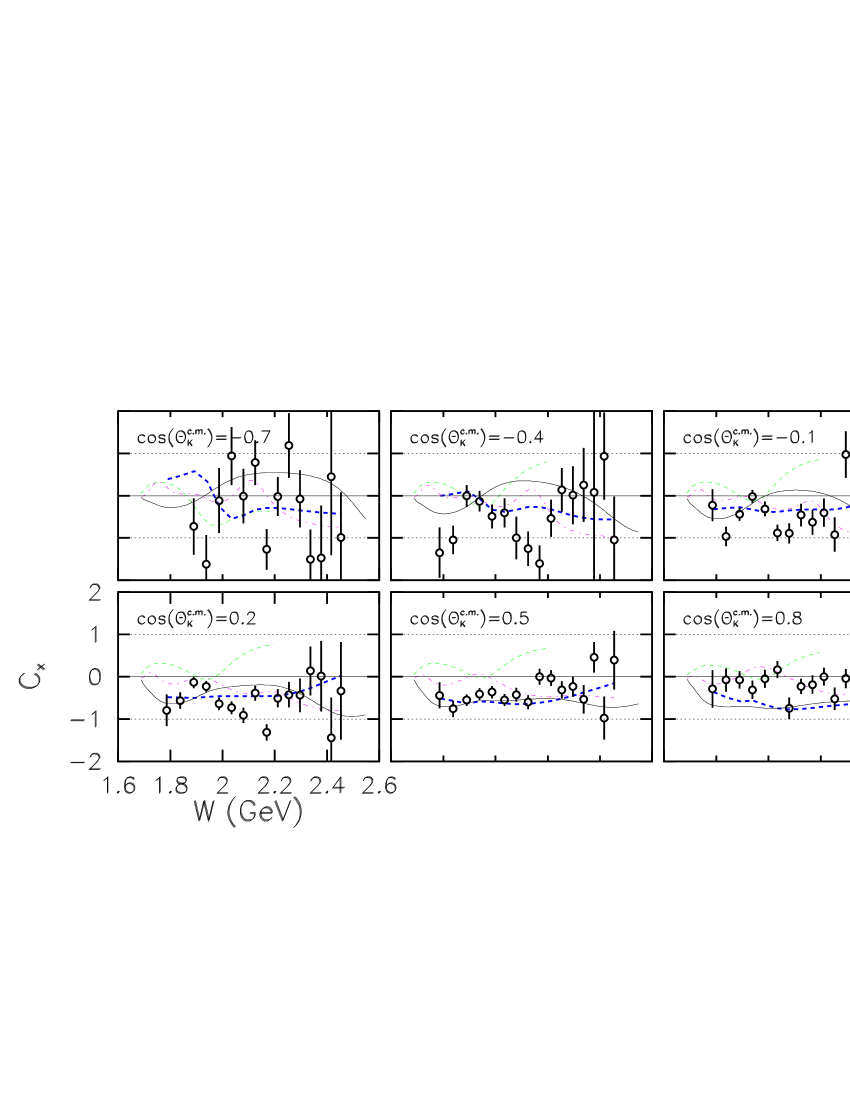
Figure 14: (Color online) The observable $C_{x}$ for the reaction $\vec{\gamma}+p\to K^{+}+\vec{\Sigma}^{0}$, plotted as a function of the c.m. energy $W$. The circles are the results of this measurement, with uncertainties discussed in the text. The thin dashed (green) curves are from Kaon-MAID maid , the thick dashed (blue) curves are from BG sarantsev2 , the thin solid (black) curves are from RPR corthals , and the thick dot-dashed (magenta) curves are from GENT jan .

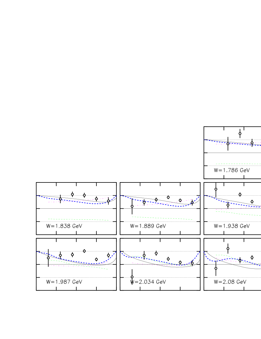
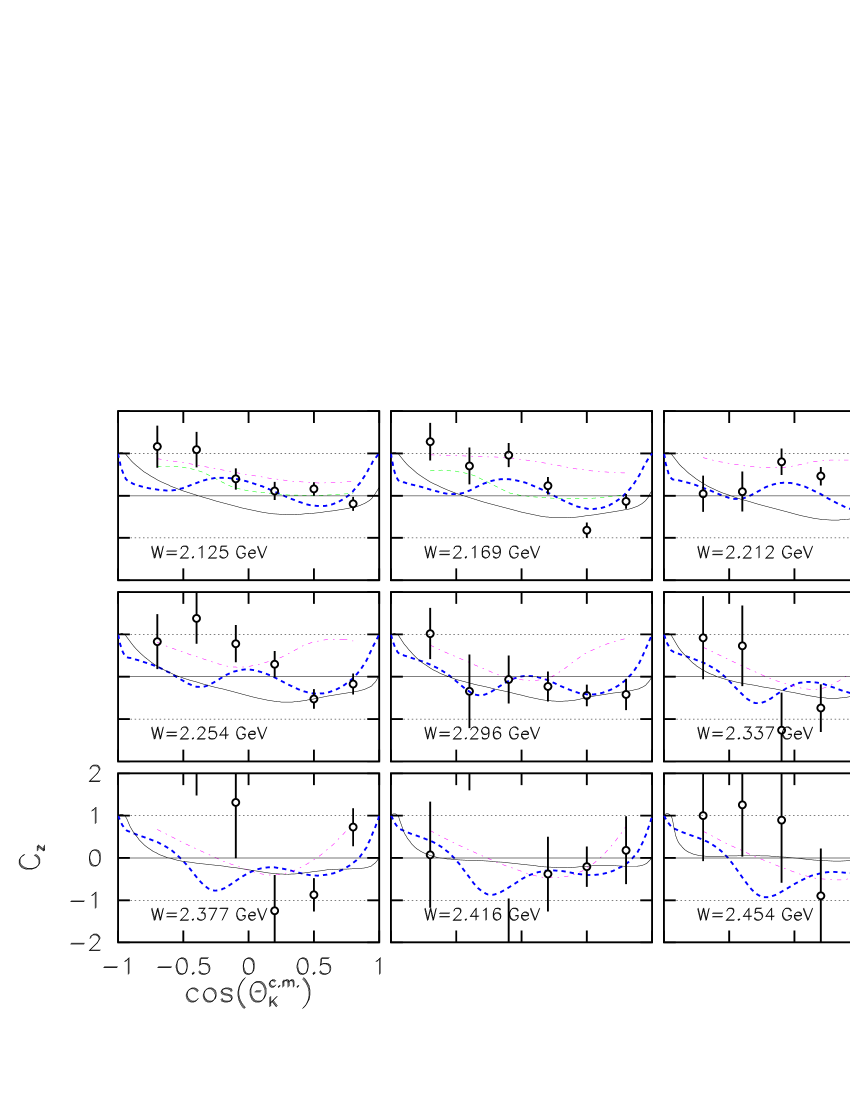
Figure 15: (Color online) The observable $C_{z}$ for the reaction $\vec{\gamma}+p\to K^{+}+\vec{\Sigma}^{0}$, plotted as a function of the kaon angle. The 16 panels are for increasing values of $W$ in steps of about 50 MeV. The circles are the results of this measurement, with uncertainties discussed in the text. The thin dashed (green) curves are from Kaon-MAID maid , the thick dashed (blue) curves are from BG sarantsev2 , the thin solid (black) curves are from RPR corthals , and the thick dot-dashed (magenta) curves are from GENT jan .

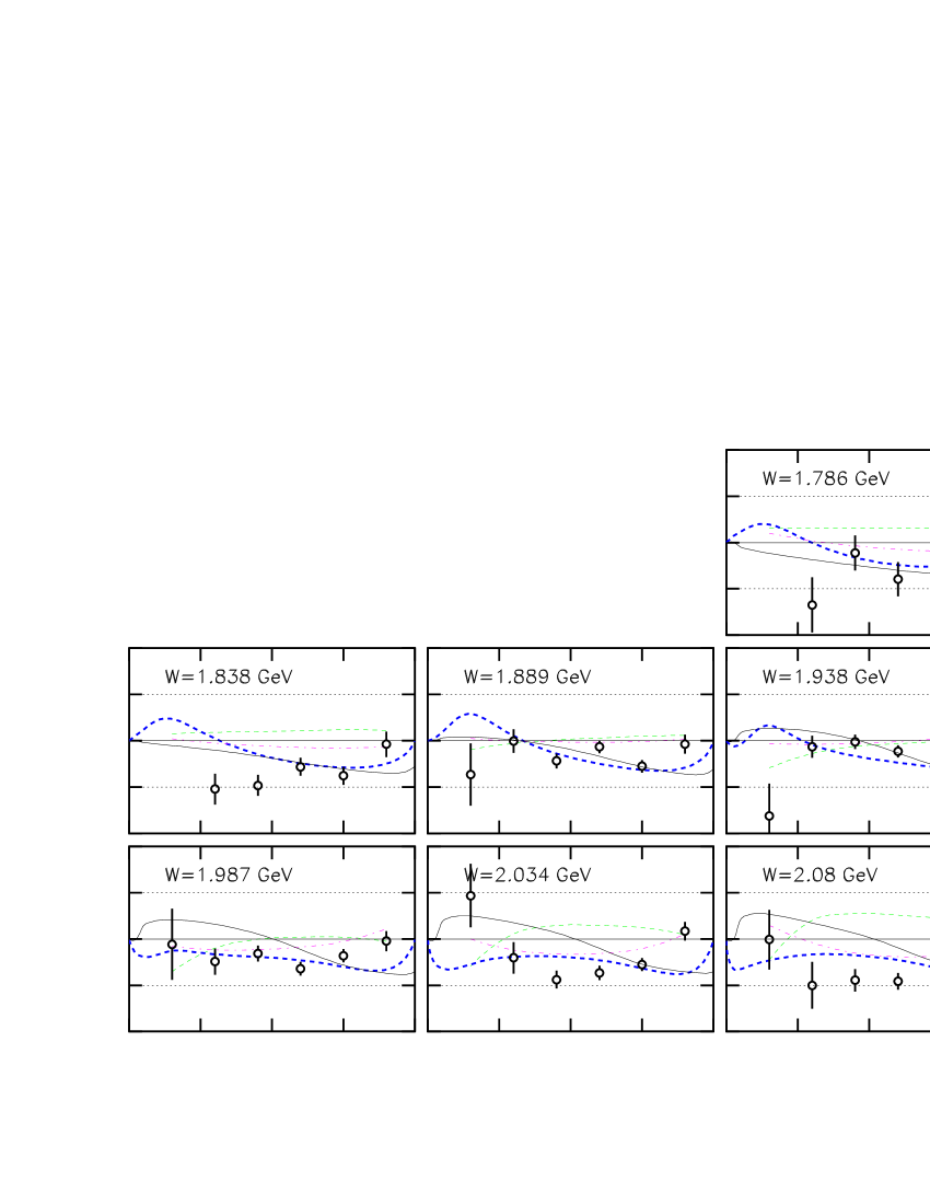
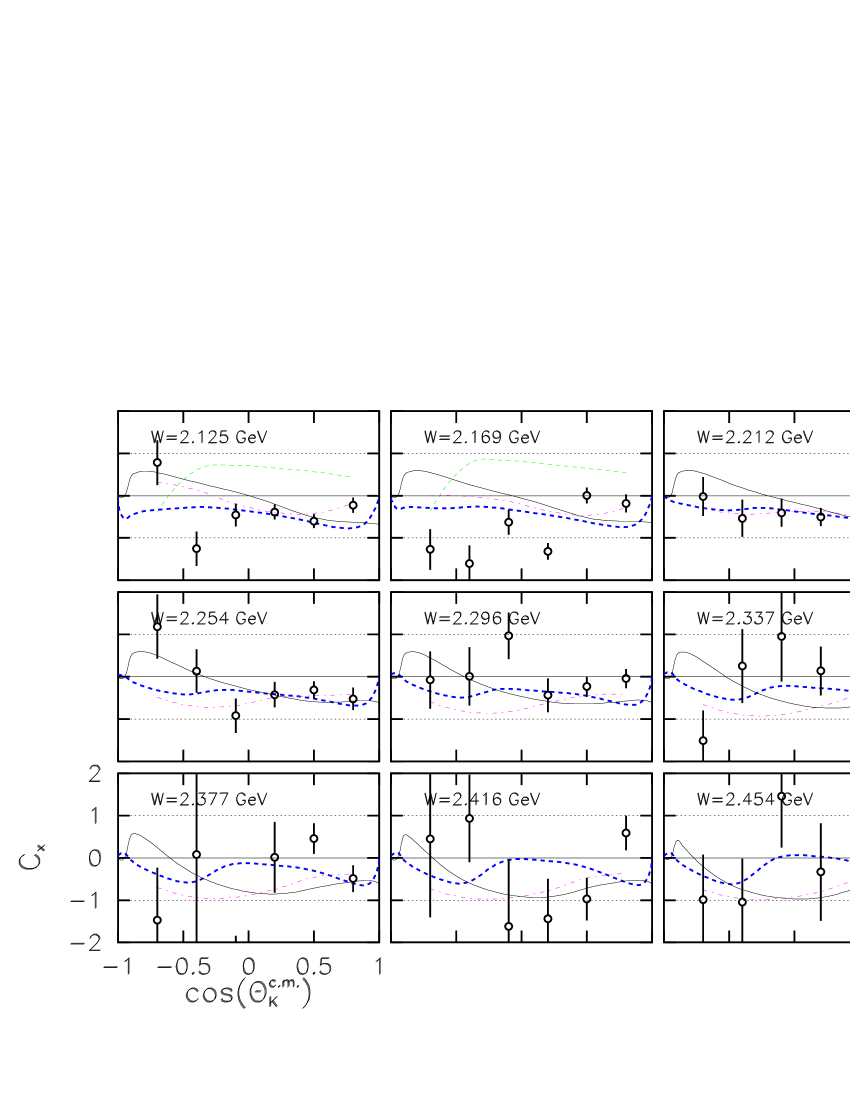
Figure 16: (Color online) The observable $C_{x}$ for the reaction $\vec{\gamma}+p\to K^{+}+\vec{\Sigma}^{0}$, plotted as a function of the kaon angle. The 16 panels are for increasing values of $W$ in steps of about 50 MeV. The circles are the results of this measurement, with uncertainties discussed in the text. The thin dashed (green) curves are from Kaon-MAID maid , the thick dashed (blue) curves are from BG sarantsev2 , the thin solid (black) curves are from RPR corthals , and the thick dot-dashed (magenta) curves are from GENT jan .

As was the case for the $\Lambda$ polarization, one expects that the magnitude of the polarization transfer coefficients, $R_{\Sigma^{0}}$, to be less than unity as per Eq. 13. The lesser statistical precision in the case of the $\Sigma^{0}$ for all three components of the combination $\{C_{x},P,C_{z}\}$ makes it more difficult to compute this precisely. However, we found that the angle and energy averaged value is

$$\overline{R}_{\Sigma^{0}}=0.82\pm.03,$$ (19)

which is clearly incompatible with the maximum possible value of unity. Thus, the $\Sigma^{0}$ cannot be said to be produced with $100\%$ polarization from a fully polarized beam. Thus, even if the quark-level dynamics leading to the creation of an $s\overline{s}$ quark pair were the same in both the $\Lambda$ and $\Sigma^{0}$ reaction channels, then the hadronization into a $\Lambda$ or a $\Sigma^{0}$ produces different final polarization states. If the quark-level dynamics are not relevant, one is left with the question of why the $\Lambda$ is formed fully spin polarized but not so the $\Sigma^{0}$.

The previous remarks about the comparison to existing reaction models apply to the $\Sigma^{0}$ case as well as the $\Lambda$ case. While none of the calculations can be said to agree well with the data, the calculation of Corthals et al. corthals at least reproduces the trend with $W$ at most angles, as shown in Fig. 13.

V.8 Further Discussion

In addition to comparison to dynamical models, as done above, one can ask what model-independent information is gained from these measurements. Photoproduction of pseudoscalar mesons from spin 1/2 baryons is described by four complex amplitudes that are functions of the reaction kinematics barker ; goldstein ; tabakin1 . For example, in the helicity basis where the photon has helicity $\pm 1$, one can easily enumerate four combinations of spins with overall helicity flips of zero ($N$), one ($S_{1}$), one ($S_{2}$), or two ($D$) units. The letter notation is that of Barker et al. barker . In a transversity basis in which the proton and hyperon have well-defined spin projections with respect to the $\hat{y}$ axis normal to the reaction plane there are linear combinations of the helicity amplitudes which are more convenient for studying polarization observables barker ; adelseck ; tabakin1 ; they are labeled $b_{1},b_{2},b_{3},b_{4}$. As shown in Table 4, these have an advantage that measurement of the cross sections (designated $A$) plus the three single spin observables $\Sigma$, $T$, $P$, yields the magnitudes of these four amplitudes. The double spin observables serve to define the three phases among the amplitudes. We note in passing that four CGLN amplitudes cgln form yet another set of amplitudes that could be used knoechlein . Table 4 shows the algebraic relations among the helicity and transversity amplitudes for the observables in hyperon photoproduction presented in this paper. At each value of Mandelstam $s$ and $t$ there are seven real numbers and an arbitrary overall phase which specify the scattering matrix. All observable quantities are expressible as bilinear products of the amplitudes, and thus there are 16 observables.

Table 4: Amplitude combinations leading to the measured observables in the helicity and transversity representations, adapted from Ref. barker . The axis convention is taken from that reference, and is rotated from the one in this paper, as discussed in the text.

Observable	Helicity	Transversity
	Representation	Representation
$A$, $d\sigma/dt$	$|N|^{2}+|S_{1}|^{2}+|S_{2}|^{2}+|D|^{2}$	$|b_{1}|^{2}+|b_{2}|^{2}+|b_{3}|^{2}+|b_{4}|^{2}$
$P$ $d\sigma/dt$	$2Im(S_{2}N^{*}-S_{1}D^{*})$	$|b_{1}|^{2}-|b_{2}|^{2}+|b_{3}|^{2}-|b_{4}|^{2}$
$C_{x^{\prime}}$ $d\sigma/dt$	$-2Re(S_{2}N^{*}+S_{1}D^{*})$	$2Im(b_{1}b_{4}^{*}-b_{2}b_{3}^{*})$
$C_{z^{\prime}}$ $d\sigma/dt$	$|S_{2}|^{2}-|S_{1}|^{2}-|N|^{2}+|D|^{2}$	$-2Re(b_{1}b_{4}^{*}+b_{2}b_{3}^{*})$

Barker et al. barker discuss which combinations of measured observables lead to complete determination of the amplitudes free of discrete ambiguities. In addition to the four measurements $A$, $\Sigma$, $T$, and $P$ they found that five double-spin observables were needed, with no four of them coming from the same set of Beam-Target, Beam-Recoil, or Target-Recoil observables. Chiang and Tabakin showed tabakin1 , however, that with careful selection of observables, a full determination of the amplitudes is possible with only four double polarization observable measurements. Still, this calls for a far-reaching program to measure the three single spin observables and at least four double spin observables chosen correctly from the available 12. According to the results in Ref. tabakin1 , the present measurements of $C_{x}$ and $C_{z}$ can be combined with almost any other pair of double spin observables to attain the desired full separation.

At present the only well-measured quantities for hyperons are the cross sections bradforddsdo ; bonn2 , induced recoil polarization $P$ mcnabb ; bonn2 ; graal , beam asymmetry $\Sigma$ leps , and the present results for $C_{x}$ and $C_{z}$. In the future, CLAS results are expected for $\Sigma$, $O_{x}$, $O_{z}$, and, pending the operation of a suitable polarized target frost , all the remaining double-spin observables. Thus, one cannot expect the present set of measurements to uniquely specify any of the underlying production amplitudes, but manipulation of the expressions in Table 4 reveals how much is accessible, in principle, from the information available with these new results. In the transversity representation, for example, let $b_{i}=r_{i}e^{-i\phi_{i}}$ and let $A$ represent the reduced cross section. Then one sees immediately that

$$A+P=2(r_{1}^{2}+r_{3}^{2})$$ (20)

$$A-P=2(r_{2}^{2}+r_{4}^{2}),$$ (21)

and after some algebra we find

$$\frac{C_{z^{\prime}}^{2}-C_{x^{\prime}}^{2}}{C_{z^{\prime}}^{2}+C_{x^{\prime}}^{2}}=\cos 2(\phi_{2}-\phi_{3})=\cos 2(\phi_{4}-\phi_{1}).$$ (22)

The latter statement is true if we select

$$(\phi_{1}+\phi_{2})-(\phi_{3}+\phi_{4})\equiv 0$$ (23)

to fix the overall phase. From present results, one thus obtains only the sums of squared magnitudes of pairs of amplitudes, and the difference between two pairs of phases. Similar expressions are obtained in the helicity representation. Thus, while a few constraints are placed on the amplitudes by these measurements, more information is needed to make the measurements a “complete” set.

VI CONCLUSIONS

In summary, we have presented results from an experimental investigation of the beam-recoil polarization observables $C_{x}$ and $C_{z}$ for $\Lambda$ and $\Sigma^{0}$ hyperon photoproduction from the proton, in the energy range from threshold through the nucleon resonance region. These are the first measurements of these observables. It is notable that the $\hat{z}$ component of $\Lambda$ polarization transfer is large and positive, indeed near $+1.0$, over a broad range of kinematics, where $\hat{z}$ is the direction of the initial state photon circular polarization. It is remarkable that the $\Lambda$ hyperon is produced fully polarized at all values of $W$ and scattering angle for a fully circularly polarized beam. The direction of this polarization is mostly along $\hat{z}$, but we have shown how $C_{x}$ and $P$ also are substantial in some kinematic regions. This phenomenon signifies some as yet unidentified dynamics in the photoproduction of strangeness. The $\Sigma^{0}$ hyperon was measured with lesser precision, but it is clear that it does not exhibit the same qualitative behavior, which is perhaps not a surprise since the spin structure of the $\Sigma^{0}$ and $\Lambda$ are different. There are no existing hadrodynamic or Regge models that do a good job of predicting these results, so it can be expected that reconsideration of these models in view of these new results may lead to new insights into the dynamics of strange quark photoproduction.

Appendix A Proton Angular Distribution in the $\Sigma^{0}$ Rest Frame

We compute the angular distribution of protons resulting from the decay of polarized $\Sigma^{0}$ ground state hyperons in the $\Sigma^{0}$ rest frame. The $\Sigma^{0}$ hyperon decays 100% according to

$$\Sigma^{0}\to\gamma+\Lambda$$ (24)

and the $\Lambda$ decays with a 64% branch via

$$\Lambda\to\pi^{-}+p.$$ (25)

A $\Sigma^{0}$ produced in a given reaction will generally be polarized to some degree, $\vec{P}_{\Sigma^{0}}$, and the $\Lambda$ arising in the decay will preserve part of the polarization. In the rest frame of the $\Lambda$ hyperon, we have the well-known parity-violating mesonic weak decay asymmetry that allows measurement of the polarization of the $\Lambda$ hyperon. For $\Lambda$ polarization component, $P_{\Lambda i}$, along a given axis in space, where $i\in\{x,y,z\}$, the proton intensity distribution, $I(\cos\theta_{pi})$, as a function of polar angle $\theta_{pi}$ is given by

$$I(\cos\theta_{pi})=\textstyle\frac{1}{2}(1+\alpha P_{\Lambda}\cos\theta_{pi}),$$ (26)

where the value of the weak decay asymmetry parameter, $\alpha$, is 0.642 pdg06 . This phenomenon arises from the interference of the parity violating $S$ and parity conserving $P$ -wave decay amplitudes perkins . To determine the $\Lambda$ polarization component, $P_{\Lambda i}$, one computes the distribution of protons with respect to $\cos\theta_{pi}$, and then determines the slope of the resulting straight line that is proportional to $P_{\Lambda i}$. This procedure must be performed in the $\Lambda$ rest frame.

In the rest frame of a $\Sigma^{0}$ hyperon the first decay is always a magnetic dipole $(M1)$ transition to a photon and a $\Lambda$. The $\Sigma^{0}$, with $J^{\pi}=1/2^{+}$, decays to a $\Lambda$ with $J^{\pi}=1/2^{+}$, and a photon with $J^{\pi}=1^{-}$. This is shown schematically in Fig. 17. As discussed below, for a given $\Sigma^{0}$ polarization axis it can be shown that the angular distribution of this decay is isotropic in the decay angle $\theta_{\Lambda}$. Crucial for this discussion is that the decay $\Lambda$ is polarized in an angle-dependent way. If the parent $\Sigma^{0}$ has polarization $\vec{P}_{\Sigma^{0}}$, then the daughter $\Lambda$ has polarization $\vec{P}_{\Lambda}$ given by

$$\vec{P}_{\Lambda}(\theta_{\Lambda})=-|\vec{P}_{\Sigma^{0}}|(\hat{z}\cdot\hat{\beta}_{\Lambda})\hat{\beta}_{\Lambda},$$ (27)

where $\vec{\beta}_{\Lambda}$ is the velocity vector of the $\Lambda$ in the $\Sigma^{0}$ rest frame. This relationship arises from evaluating the expectation value of the spin operator of the $\Lambda$ in terms of the transition matrix for this electromagnetic decay gatto ; dreitlein . This equation says that the $\Lambda$ is polarized along the axis it is emitted, with its magnitude scaled by the cosine of the emission angle, $\theta_{\Lambda}$, as indicated in the figure.

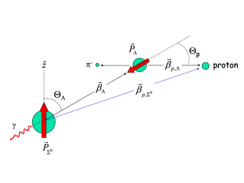
Figure 17: (Color online) The $\Sigma^{0}$ hyperon, polarized along the $\hat{z}$ axis, decays to a $\gamma$ and a $\Lambda$ at some angle $\theta_{\Lambda}$. The $\Lambda$ is polarized as shown, traveling at speed $\beta_{\Lambda}$. In the $\Lambda$ rest frame, the $\Lambda$ decays into a $\pi^{-}$ and a proton, where the proton emission angle with respect to $\hat{\beta}_{\Lambda}$ is $\theta_{p}$ and the speed of the proton is $\beta_{p,\Lambda}$.

In the $\Lambda$ rest frame, then, the decay angular distribution of the protons can be written

$$I(\hat{\beta}_{p,\Lambda})=c(1-\alpha P_{\Sigma^{0}}(\hat{z}\cdot\hat{\beta}_{\Lambda})(\hat{\beta}_{\Lambda}\cdot\hat{\beta}_{p,\Lambda})),$$ (28)

where $c$ is a normalization constant, or equivalently as

$$I(\cos\theta_{p})=c(1-\alpha P_{\Sigma^{0}}\cos\theta_{\Lambda}\cos\theta_{p}).$$ (29)

In situations where the photons are not detected, and the acceptance for the $\Lambda$ decay products is taken into account properly, we can integrate over all values of $\theta_{\Lambda}$. The only direction along which to measure an asymmetry is then $\hat{z}$, and we must measure the proton angle from this axis, which we will call $\theta_{p,\Sigma^{0}}$; this projection introduces another factor of $\cos\theta_{\Lambda}$. The solid-angle weighted average of $\cos^{2}\theta_{\Lambda}$ is $1/3$, leading to the equation

$$I_{avg}(\theta_{p,\Sigma^{0}})=c(1-\alpha P_{\Sigma^{0}}\frac{1}{3}\cos\theta_{p,\Sigma^{0}})$$ (30)

for the average distribution of protons in the $\Lambda$ hyperon rest frame. Thus, if the direction of the $\Lambda$ is not explicitly measured, the effective polarization component of the $\Lambda$ reduces along $\hat{z}$ to the relationship

$$P_{\Lambda}=-\frac{1}{3}P_{\Sigma^{0}}.$$ (31)

As a mnemonic, one can say that the average $\Lambda$ polarization is $-1/3$ of the $\Sigma^{0}$ polarization. However, this statement is true only in the sense of averaging over all possible $\Lambda$ emission angles.

Now we reach the statement of the problem at hand: what is the angular distribution of the protons from the decay of the $\Lambda$’s when measured in the $\Sigma^{0}$ rest frame instead of the $\Lambda$ rest frame? That is, how can the polarization of the parent $\Sigma^{0}$ be determined without boosting the protons to the rest frame of the $\Lambda$? This problem arises, for example, in the case of the fixed-target reaction

$$\gamma+p \to K^{+}+\vec{\Sigma}^{0}$$

$$\to K^{+}+(\gamma)+\vec{\Lambda}$$

$$\to K^{+}+(\gamma)+(\pi^{-})+p,$$

where the particles in parentheses are not detected and the vectors designate the polarized hyperons. The photon and the kaon define the boost to the $\Sigma^{0}$ rest frame, but without detecting the $\gamma$ or the $\pi^{-}$ it is impossible to define the boost to the $\Lambda$ rest frame. Determination of the induced or transferred polarizations of the $\Sigma^{0}$ necessitates using the angular distribution of the protons in the $\Sigma^{0}$ frame. There is enough kinematic definition to boost the detected proton to the $\Sigma^{0}$ rest frame, hence we need to compute the expected angular distribution of the protons in that frame.

A.1 The Calculations

The polarization of the parent $\Sigma^{0}$ particle is the expectation value of the Pauli spin operator, $P_{\Sigma^{0}}=<\vec{\sigma}>_{\Sigma}$. In a basis where the initial polarization direction is the quantization axis, the $\Lambda$ spin either is flipped or is not flipped relative to the $\Sigma^{0}$ spin. If the parent particle is in the $m_{\Sigma}=+1/2$ state, then it can be shown that the non-spin flip transition leads to an angular distribution, $I_{+1/2}$, proportional to $(1-\cos^{2}\theta_{\Lambda})$. The angular distribution for spin flip, $I_{-1/2}$, is proportional to $(1+\cos^{2}\theta_{\Lambda})$. Summing these two equal-strength non-interfering final states leads to two predictions. First, the net angular distribution of the $\Lambda$’s in the $\Sigma^{0}$ rest frame is isotropic, namely

$$I(\theta_{\Lambda})\sim I_{+1/2}+I_{-1/2}\sim 1.$$ (33)

Second, the polarization of the $\Lambda$ hyperons is given by

$$P_{\Lambda}(\theta_{\Lambda})=P_{\Sigma^{0}}\frac{I_{+1/2}-I_{-1/2}}{I_{+1/2}+I_{-1/2}}=-P_{\Sigma^{0}}\cos^{2}{\theta_{\Lambda}}$$ (34)

as stated in the introduction. Integration of the $I_{m}(\theta_{\Lambda})$’s over all values of $\theta_{\Lambda}$ leads to the result that 1/3 of the time the transition does not flip the spin (i.e. $m_{\Lambda}=+1/2$), while 2/3 of the time the transition flips the spin $(m_{\Lambda}=-1/2)$. The net average polarization of the $\Lambda$ along the initial polarization axis is then $-1/3$ of the parent $\Sigma^{0}$ polarization. We have done the detailed calculation of these results ourselves, and found corroboration in several places gatto ; dreitlein ; tabakin2 . However, the calculation of the proton distribution in the $\Sigma^{0}$ rest frame requires additional considerations.

In the $\Sigma^{0}$ rest frame the $\Lambda$ and $\gamma$ are produced with a momentum of 74.48 MeV/c, which corresponds to a speed of the $\Lambda$ of $\beta_{\Lambda}=0.0666$. In the $\Lambda$ rest frame the proton and the $\pi^{-}$ are produced with a momentum of 100.58 MeV/c, which corresponds to a speed of the proton of $\beta_{p}=0.1072$. Thus, both the $\Lambda$ and the proton are non-relativistic in the $\Sigma^{0}$ rest frame, so we will treat the frame transformation in terms of simple non-relativistic velocity addition. That is, we compute a weighted average over all possible $\Lambda$ velocities in the $\Sigma^{0}$ frame, $\vec{\beta}_{\Lambda}$, and all proton velocities in the $\Lambda$ frame, $\vec{\beta}_{p,\Lambda}$:

$$\vec{\beta}_{p,\Sigma^{0}}=\vec{\beta}_{p,\Lambda}+\vec{\beta}_{\Lambda}.$$ (35)

This can be computed either with an explicit numerical integration or by integration using a Monte Carlo technique.

A.1.1 Explicit Integration

To compute the proton distribution in the $\Sigma^{0}$ rest frame, $I_{p}(\cos\theta_{p,{\Sigma^{0}}})$, by means of an integration over all possible proton and $\Lambda$ orientations, each angle combination must be properly weighted by the underlying intensity distribution and the proper differential area element. As discussed above, the decay-$\Lambda$ distribution is isotropic, and so the density in three dimensions is equal to $1/4\pi$. The proton distribution in the $\Lambda$ rest frame in three dimensions is given by $(1/2\pi)I(\theta_{p})$, where $I(\theta_{p})$ is given by Eq. 29.

We take the initial polarization, $P_{\Sigma^{0}}$, to be 100%. The complete expression for evaluating the proton angular distribution in the $\Sigma^{0}$ rest frame is

$$I_{p}(\cos\theta_{p,{\Sigma^{0}}})=\int_{\theta_{\Lambda}=0}^{\pi}\frac{1}{4\pi}\int_{\theta_{p}=0}^{\pi}\int_{\phi_{p}=0}^{2\pi}\delta(\vec{\beta}_{p,\Sigma^{0}}(\theta_{p,\Sigma^{0}})-(\vec{\beta}_{\Lambda}(\theta_{\Lambda})+\vec{\beta}_{p,\Lambda}(\theta_{p},\phi_{p}))$$

$$\times\textstyle\frac{1}{2}\left(1+\alpha(-\cos^{2}\theta_{\Lambda})\cos\theta_{p}\right)d\phi_{p}\sin\theta_{p}d\theta_{p}\sin\theta_{\Lambda}d\theta_{\Lambda}.$$ (36)

The delta function formally enforces the requirement of selecting all those vector combinations of velocities which lead to a given value of the proton angle in the $\Sigma^{0}$ rest frame. In practice, the integral was evaluated by numerically sweeping over all values of $\theta_{p}$, $\phi_{p}$, and $\theta_{\Lambda}$, and accumulating the distribution of proton angles in the $\Sigma^{0}$ rest frame, $\theta_{p,\Sigma^{0}}$, with the weighting given by the rest of the integrand.

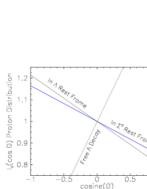
Figure 18: (Color online) The solid (blue) line shows the proton angular distribution in the $\Sigma^{0}$ rest frame, where $\theta$ is the polar angle with respect to the polarization axis $\hat{z}$. The dashed (black) line shows the expected slope of the proton distribution in the $\Lambda$ rest frame, where the angle $\theta$ in the graph is construed as the proton angle $\theta_{p}$, i.e. measured from the axis of the $\Lambda$’s velocity. The dotted (black) curve shows, for reference, the slope of the proton distribution in the case of fully polarized $\Lambda$ hyperons decaying, where the angle is $\theta_{p}$ with respect to the $\Lambda$ polarization axis.

The result is shown in Fig. 18. The calculation assumes a fully polarized $\Sigma^{0}$ hyperon. The solid line shows the result of the integration. In effect, the straight-line proton distribution in the $\Lambda$ rest frame (dot-dashed line) is shifted by the transformation to the $\Sigma^{0}$ rest frame. The fact that this result is a straight line rather than some inflected curve is significant. It shows that the $\Sigma^{0}$ polarization can be determined using the same method, in essence, as when determining a $\Lambda$’s polarization. Experimental data can be fitted with this slope and the actual polarization of the parent particle can be deduced from the scale factor. The first moment of the calculated distribution gives the slope. The value is $-0.1646$ in the $\Sigma^{0}$ rest frame. In the rest frame of the $\Lambda$, when all possible decay-$\Lambda$ angles are averaged the slope is given by $-(1/3)\alpha=-0.214$. Thus, the slope of the asymmetry is reduced by the frame transformation by an amount given by $1/(.2140/.1646)=1/1.300=0.769$. Thus, one can say the frame transformation reduces the slope by 30.0%, or alternatively, that the effective weak decay constant, $\alpha_{eff}$ is

$$\alpha_{eff}=-\alpha\times 0.256=\alpha\times\left(-\frac{1}{3.90}\right).$$ (37)

A.1.2 Monte Carlo Simulation

Two separate three-dimensional Monte Carlo simulations of the problem were performed. The frame-transformation calculation was treated non-relativistically, as in the explicit integration discussed in the previous section. The difference in approach entailed random weighted selection of the decay directions at each step, which eliminated the need to separately compute the solid-angle weighting factors. The results of the Monte Carlo and of the direct numerical integration methods agreed to three significant figures.

A.2 Appendix Summary

Using two independent calculation methods we have numerically evaluated the angular distribution of protons that arise from the two-step decay of $\Sigma^{0}$ hyperons in their rest frame. The result is a decay asymmetry that is well represented by a constant slope in $\cos{\theta_{p,{\Sigma^{0}}}}$. The distribution has a slope that is reduced by 30.0% with respect to the average slope expected in the rest frame of the intermediate $\Lambda$ hyperon. The effective weak decay constant is $-0.165$.

Appendix B Numerical Data

The polarization transfer results from the present work are given below. Each row gives the values for $C_{x}$ and $C_{z}$ for the stated values of photon energy and $\cos\theta_{K^{+}}^{c.m.}$, where $\theta_{K^{+}}^{c.m.}$ is the center-of-mass angle of the kaon. The quoted uncertainties are the statistical errors resulting from the proton yield asymmetry fitting combined with the point-to-point systematic uncertainty in the fitting procedures. Global systematic uncertainties were discussed in the main text. A zero value for an uncertainty means that no data point was extracted at that energy and angle. Electronic tabulations of the results are available from several archival sources bradfordthesis , clasdb , durham , contact .

Table 5: Results of CLAS measurements of $\gamma+p\to K^{+}+\Lambda$. The columns marked $C_{x}$ and $C_{z}$ are the polarization transfer coefficients of the photon to the hyperon in the $\gamma p$ center-of-mass (c.m.) frame, where $\hat{x}$ and $\hat{z}$ are defined in the text. The column $\cos\theta_{K^{+}}^{c.m.}$ gives the c.m. angle of the produced $K^{+}$ meson. The columns marked $\delta C_{x}$ and $\delta C_{z}$ are the associated uncertainties.

Index	$E_{\gamma}$	W	$\cos\theta_{K}^{c.m.}$	$C_{x}$	$\delta{C_{x}}$	$C_{z}$	$\delta C_{z}$
	(GeV)	(GeV)
1)	1.032	1.679	-0.75	0.000	0.000	0.000	0.000
2)	1.032	1.679	-0.55	0.114	0.724	0.698	0.542
3)	1.032	1.679	-0.35	-0.960	0.269	0.686	0.230
4)	1.032	1.679	-0.15	-0.304	0.186	0.812	0.172
5)	1.032	1.679	0.05	-0.470	0.169	0.917	0.160
6)	1.032	1.679	0.25	-0.700	0.175	0.838	0.154
7)	1.032	1.679	0.45	-0.444	0.139	0.555	0.131
8)	1.032	1.679	0.65	-0.216	0.154	0.821	0.135
9)	1.032	1.679	0.85	-0.126	0.190	0.901	0.189
10)	1.132	1.734	-0.75	0.000	0.000	0.000	0.000
11)	1.132	1.734	-0.55	-0.453	0.310	0.451	0.280
12)	1.132	1.734	-0.35	-0.543	0.186	0.742	0.179
13)	1.132	1.734	-0.15	-0.260	0.136	0.940	0.135
14)	1.132	1.734	0.05	-0.301	0.123	1.004	0.117
15)	1.132	1.734	0.25	-0.426	0.108	0.983	0.110
16)	1.132	1.734	0.45	-0.235	0.089	0.752	0.085
17)	1.132	1.734	0.65	-0.189	0.103	0.893	0.084
18)	1.132	1.734	0.85	-0.262	0.160	1.017	0.111
19)	1.232	1.787	-0.75	0.140	1.021	0.974	0.426
20)	1.232	1.787	-0.55	-0.224	0.228	1.002	0.205
21)	1.232	1.787	-0.35	-0.065	0.138	0.762	0.140
22)	1.232	1.787	-0.15	-0.375	0.112	0.848	0.113
23)	1.232	1.787	0.05	0.041	0.097	0.779	0.102
24)	1.232	1.787	0.25	-0.185	0.081	0.983	0.088
25)	1.232	1.787	0.45	-0.072	0.069	0.905	0.087
26)	1.232	1.787	0.65	-0.061	0.069	1.021	0.077
27)	1.232	1.787	0.85	-0.086	0.094	1.001	0.100
28)	1.332	1.839	-0.75	0.024	0.303	0.982	0.238
29)	1.332	1.839	-0.55	-0.094	0.148	0.869	0.146
30)	1.332	1.839	-0.35	-0.237	0.109	1.067	0.112
31)	1.332	1.839	-0.15	-0.160	0.089	1.067	0.094
32)	1.332	1.839	0.05	-0.056	0.081	0.891	0.098
33)	1.332	1.839	0.25	-0.086	0.067	0.943	0.074
34)	1.332	1.839	0.45	-0.139	0.063	1.016	0.066
35)	1.332	1.839	0.65	-0.044	0.062	0.998	0.064
36)	1.332	1.839	0.85	0.015	0.081	0.998	0.080
37)	1.433	1.889	-0.75	-0.099	0.155	1.125	0.149
38)	1.433	1.889	-0.55	-0.266	0.106	0.954	0.117
39)	1.433	1.889	-0.35	-0.145	0.097	1.203	0.101
40)	1.433	1.889	-0.15	0.050	0.078	1.044	0.086
41)	1.433	1.889	0.05	-0.074	0.070	0.900	0.080
42)	1.433	1.889	0.25	-0.047	0.058	1.076	0.069
43)	1.433	1.889	0.45	-0.149	0.053	0.881	0.066
44)	1.433	1.889	0.65	-0.218	0.050	0.966	0.063
45)	1.433	1.889	0.85	-0.038	0.067	1.075	0.076
46)	1.534	1.939	-0.75	-0.086	0.129	0.914	0.124
47)	1.534	1.939	-0.55	-0.104	0.115	0.723	0.105
48)	1.534	1.939	-0.35	-0.047	0.093	1.062	0.096
49)	1.534	1.939	-0.15	-0.027	0.080	0.928	0.084
50)	1.534	1.939	0.05	0.003	0.070	0.910	0.074
51)	1.534	1.939	0.25	0.002	0.054	0.886	0.063
52)	1.534	1.939	0.45	-0.076	0.047	0.853	0.058
53)	1.534	1.939	0.65	-0.191	0.046	1.011	0.054
54)	1.534	1.939	0.85	-0.084	0.060	1.051	0.066
55)	1.635	1.987	-0.75	-0.216	0.155	0.554	0.141
56)	1.635	1.987	-0.55	-0.058	0.135	0.632	0.129
57)	1.635	1.987	-0.35	-0.140	0.116	0.731	0.123
58)	1.635	1.987	-0.15	-0.014	0.112	0.897	0.097
59)	1.635	1.987	0.05	0.226	0.080	1.001	0.078
60)	1.635	1.987	0.25	-0.105	0.059	0.829	0.062
61)	1.635	1.987	0.45	-0.128	0.054	0.925	0.053
62)	1.635	1.987	0.65	-0.319	0.049	0.941	0.054
63)	1.635	1.987	0.85	-0.195	0.073	0.893	0.107
64)	1.737	2.035	-0.75	-0.121	0.145	0.472	0.136
65)	1.737	2.035	-0.55	-0.497	0.149	0.229	0.149
66)	1.737	2.035	-0.35	-0.305	0.141	0.554	0.163
67)	1.737	2.035	-0.15	-0.168	0.110	0.608	0.115
68)	1.737	2.035	0.05	-0.010	0.081	0.801	0.089
69)	1.737	2.035	0.25	0.120	0.063	0.843	0.064
70)	1.737	2.035	0.45	-0.112	0.050	1.022	0.057
71)	1.737	2.035	0.65	-0.241	0.055	0.886	0.047
72)	1.737	2.035	0.85	-0.331	0.071	0.942	0.090
73)	1.838	2.081	-0.75	-0.384	0.180	0.422	0.174
74)	1.838	2.081	-0.55	-0.618	0.189	0.207	0.192
75)	1.838	2.081	-0.35	-0.960	0.190	0.469	0.189
76)	1.838	2.081	-0.15	-0.056	0.139	0.489	0.150
77)	1.838	2.081	0.05	0.229	0.107	0.989	0.112
78)	1.838	2.081	0.25	0.087	0.071	0.850	0.080
79)	1.838	2.081	0.45	-0.109	0.056	0.946	0.068
80)	1.838	2.081	0.65	-0.335	0.065	0.831	0.103
81)	1.838	2.081	0.85	-0.448	0.074	0.870	0.063
82)	1.939	2.126	-0.75	-0.522	0.182	0.778	0.174
83)	1.939	2.126	-0.55	-1.082	0.181	0.499	0.177
84)	1.939	2.126	-0.35	-0.957	0.174	0.352	0.205
85)	1.939	2.126	-0.15	-0.558	0.150	0.786	0.149
86)	1.939	2.126	0.05	-0.034	0.111	0.743	0.125
87)	1.939	2.126	0.25	0.290	0.077	0.922	0.083
88)	1.939	2.126	0.45	-0.154	0.110	1.048	0.272
89)	1.939	2.126	0.65	-0.328	0.166	0.726	0.239
90)	1.939	2.126	0.85	-0.475	0.063	0.691	0.068
91)	2.039	2.170	-0.75	-0.501	0.186	0.469	0.171
92)	2.039	2.170	-0.55	-0.962	0.161	0.533	0.175
93)	2.039	2.170	-0.35	-0.896	0.168	0.486	0.220
94)	2.039	2.170	-0.15	-0.121	0.161	0.621	0.175
95)	2.039	2.170	0.05	0.053	0.121	0.908	0.141
96)	2.039	2.170	0.25	0.078	0.088	1.045	0.092
97)	2.039	2.170	0.45	-0.047	0.068	1.045	0.196
98)	2.039	2.170	0.65	-0.431	0.062	0.834	0.061
99)	2.039	2.170	0.85	-0.552	0.061	0.655	0.071
100)	2.139	2.212	-0.75	-0.983	0.252	0.987	0.204
101)	2.139	2.212	-0.55	-0.800	0.187	0.760	0.197
102)	2.139	2.212	-0.35	-0.711	0.273	0.569	0.198
103)	2.139	2.212	-0.15	-0.170	0.180	0.425	0.231
104)	2.139	2.212	0.05	-0.145	0.131	0.858	0.158
105)	2.139	2.212	0.25	0.034	0.106	0.886	0.106
106)	2.139	2.212	0.45	0.020	0.084	1.042	0.099
107)	2.139	2.212	0.65	-0.299	0.056	0.761	0.074
108)	2.139	2.212	0.85	-0.455	0.062	0.676	0.074
109)	2.240	2.255	-0.75	-0.690	0.226	0.674	0.228
110)	2.240	2.255	-0.55	-0.466	0.268	0.962	0.231
111)	2.240	2.255	-0.35	-0.931	0.252	0.872	0.278
112)	2.240	2.255	-0.15	-0.504	0.229	0.365	0.229
113)	2.240	2.255	0.05	0.206	0.194	0.576	0.213
114)	2.240	2.255	0.25	0.245	0.136	1.080	0.138
115)	2.240	2.255	0.45	-0.183	0.098	1.061	0.130
116)	2.240	2.255	0.65	-0.466	0.077	0.698	0.081
117)	2.240	2.255	0.85	-0.421	0.075	0.576	0.087
118)	2.341	2.296	-0.75	-0.357	0.384	1.015	0.296
119)	2.341	2.296	-0.55	-0.232	0.290	0.487	0.372
120)	2.341	2.296	-0.35	-0.354	0.261	1.266	0.307
121)	2.341	2.296	-0.15	-0.241	0.320	0.502	0.326
122)	2.341	2.296	0.05	0.280	0.299	1.016	0.322
123)	2.341	2.296	0.25	0.636	0.194	0.779	0.189
124)	2.341	2.296	0.45	0.032	0.130	1.147	0.128
125)	2.341	2.296	0.65	-0.492	0.083	0.638	0.099
126)	2.341	2.296	0.85	-0.450	0.087	0.610	0.121
127)	2.443	2.338	-0.75	-0.790	0.385	0.907	0.402
128)	2.443	2.338	-0.55	-0.697	0.422	1.412	0.416
129)	2.443	2.338	-0.35	-0.253	0.402	1.025	0.472
130)	2.443	2.338	-0.15	-0.521	0.366	0.932	0.429
131)	2.443	2.338	0.05	-0.097	0.278	0.866	0.317
132)	2.443	2.338	0.25	0.107	0.231	0.499	0.293
133)	2.443	2.338	0.45	0.191	0.156	1.439	0.170
134)	2.443	2.338	0.65	-0.393	0.334	0.508	0.386
135)	2.443	2.338	0.85	-0.416	0.157	0.360	0.172
136)	2.543	2.377	-0.75	-0.393	0.432	0.396	0.410
137)	2.543	2.377	-0.55	-0.007	0.420	0.281	0.669
138)	2.543	2.377	-0.35	-0.938	0.466	1.102	0.369
139)	2.543	2.377	-0.15	-0.188	0.406	1.170	0.471
140)	2.543	2.377	0.05	-0.521	0.403	0.525	0.596
141)	2.543	2.377	0.25	-0.289	0.401	0.390	0.290
142)	2.543	2.377	0.45	-0.426	0.189	0.809	0.235
143)	2.543	2.377	0.65	-0.258	0.126	0.698	0.145
144)	2.543	2.377	0.85	-0.450	0.114	0.504	0.164
145)	2.642	2.416	-0.75	-0.135	0.569	1.640	0.497
146)	2.642	2.416	-0.55	-0.102	0.554	1.580	0.624
147)	2.642	2.416	-0.35	-0.903	0.472	1.385	0.367
148)	2.642	2.416	-0.15	-0.866	0.533	0.649	0.478
149)	2.642	2.416	0.05	-0.052	0.534	0.587	0.459
150)	2.642	2.416	0.25	0.122	0.405	-0.369	0.399
151)	2.642	2.416	0.45	-0.126	0.238	0.887	0.240
152)	2.642	2.416	0.65	-0.385	0.140	0.548	0.157
153)	2.642	2.416	0.85	-0.155	0.205	0.397	0.238
154)	2.741	2.454	-0.75	0.534	0.796	0.667	0.610
155)	2.741	2.454	-0.55	0.064	1.182	0.000	0.833
156)	2.741	2.454	-0.35	0.105	0.713	-0.517	1.211
157)	2.741	2.454	-0.15	-0.289	0.442	1.129	0.618
158)	2.741	2.454	0.05	-0.549	0.717	-0.171	0.480
159)	2.741	2.454	0.25	0.071	0.402	0.117	0.354
160)	2.741	2.454	0.45	-0.083	0.233	0.906	0.318
161)	2.741	2.454	0.65	-0.474	0.213	0.809	0.222
162)	2.741	2.454	0.85	-0.449	0.212	0.283	0.527

Table 6: Results of CLAS measurements of $\gamma+p\to K^{+}+\Sigma^{0}$. The columns marked $C_{x}$ and $C_{z}$ are the polarization transfer coefficients of the photon to the hyperon in the $\gamma p$ center-of-mass (c.m.) frame, where $\hat{x}$ and $\hat{z}$ are defined in the text. The column $\cos\theta_{K^{+}}^{c.m.}$ gives the c.m. angle of the produced $K^{+}$ meson. The columns marked $\delta C_{x}$ and $\delta C_{z}$ are the associated uncertainties.

Index	$E_{\gamma}$	W	$\cos\theta_{K}^{c.m.}$	$C_{x}$	$\delta{C_{x}}$	$C_{z}$	$\delta C_{z}$
	(GeV)	(GeV)
1)	1.232	1.787	-0.70	0.000	0.000	0.000	0.000
2)	1.232	1.787	-0.40	-1.348	0.595	0.689	0.519
3)	1.232	1.787	-0.10	-0.227	0.379	1.477	0.347
4)	1.232	1.787	0.20	-0.792	0.371	0.760	0.301
5)	1.232	1.787	0.50	-0.438	0.305	1.391	0.302
6)	1.232	1.787	0.80	-0.286	0.442	1.334	0.383
7)	1.332	1.839	-0.70	0.000	0.000	0.000	0.000
8)	1.332	1.839	-0.40	-1.045	0.335	0.734	0.325
9)	1.332	1.839	-0.10	-0.963	0.226	1.092	0.208
10)	1.332	1.839	0.20	-0.563	0.193	1.019	0.189
11)	1.332	1.839	0.50	-0.756	0.192	0.744	0.184
12)	1.332	1.839	0.80	-0.077	0.277	0.585	0.279
13)	1.433	1.889	-0.70	-0.729	0.670	0.171	0.612
14)	1.433	1.889	-0.40	-0.007	0.257	0.475	0.239
15)	1.433	1.889	-0.10	-0.437	0.157	0.681	0.156
16)	1.433	1.889	0.20	-0.131	0.137	0.866	0.138
17)	1.433	1.889	0.50	-0.552	0.139	0.632	0.135
18)	1.433	1.889	0.80	-0.074	0.205	0.458	0.220
19)	1.534	1.939	-0.70	-1.622	0.693	1.482	0.619
20)	1.534	1.939	-0.40	-0.131	0.238	0.262	0.267
21)	1.534	1.939	-0.10	-0.020	0.156	1.075	0.162
22)	1.534	1.939	0.20	-0.227	0.134	0.528	0.142
23)	1.534	1.939	0.50	-0.410	0.140	0.706	0.148
24)	1.534	1.939	0.80	-0.309	0.218	0.351	0.205
25)	1.635	1.987	-0.70	-0.115	0.767	0.497	0.677
26)	1.635	1.987	-0.40	-0.490	0.283	0.697	0.281
27)	1.635	1.987	-0.10	-0.312	0.173	0.744	0.185
28)	1.635	1.987	0.20	-0.640	0.147	1.022	0.141
29)	1.635	1.987	0.50	-0.362	0.143	0.379	0.146
30)	1.635	1.987	0.80	-0.047	0.216	0.697	0.186
31)	1.737	2.035	-0.70	0.936	0.683	-0.965	0.592
32)	1.737	2.035	-0.40	-0.406	0.341	0.693	0.328
33)	1.737	2.035	-0.10	-0.878	0.195	0.854	0.194
34)	1.737	2.035	0.20	-0.731	0.153	0.419	0.149
35)	1.737	2.035	0.50	-0.550	0.139	0.149	0.141
36)	1.737	2.035	0.80	0.168	0.201	0.097	0.228
37)	1.838	2.081	-0.70	-0.011	0.644	-0.303	0.579
38)	1.838	2.081	-0.40	-1.000	0.507	1.215	0.386
39)	1.838	2.081	-0.10	-0.891	0.240	0.319	0.232
40)	1.838	2.081	0.20	-0.912	0.179	0.524	0.178
41)	1.838	2.081	0.50	-0.429	0.164	0.048	0.148
42)	1.838	2.081	0.80	-0.745	0.253	-0.082	0.178
43)	1.939	2.126	-0.70	0.782	0.529	1.157	0.493
44)	1.939	2.126	-0.40	-1.255	0.403	1.089	0.417
45)	1.939	2.126	-0.10	-0.458	0.264	0.397	0.249
46)	1.939	2.126	0.20	-0.388	0.176	0.111	0.213
47)	1.939	2.126	0.50	-0.601	0.166	0.159	0.155
48)	1.939	2.126	0.80	-0.227	0.182	-0.193	0.164
49)	2.039	2.170	-0.70	-1.268	0.480	1.279	0.444
50)	2.039	2.170	-0.40	-1.606	0.430	0.700	0.434
51)	2.039	2.170	-0.10	-0.629	0.294	0.958	0.284
52)	2.039	2.170	0.20	-1.315	0.196	0.235	0.208
53)	2.039	2.170	0.50	0.004	0.188	-0.818	0.182
54)	2.039	2.170	0.80	-0.185	0.216	-0.134	0.170
55)	2.139	2.212	-0.70	-0.019	0.457	0.047	0.429
56)	2.139	2.212	-0.40	-0.535	0.438	0.098	0.471
57)	2.139	2.212	-0.10	-0.405	0.332	0.800	0.314
58)	2.139	2.212	0.20	-0.507	0.214	0.462	0.219
59)	2.139	2.212	0.50	-0.029	0.183	-0.100	0.188
60)	2.139	2.212	0.80	0.002	0.209	-0.041	0.163
61)	2.240	2.255	-0.70	1.186	0.761	0.828	0.649
62)	2.240	2.255	-0.40	0.134	0.515	1.377	0.600
63)	2.240	2.255	-0.10	-0.920	0.404	0.783	0.440
64)	2.240	2.255	0.20	-0.424	0.300	0.294	0.310
65)	2.240	2.255	0.50	-0.312	0.203	-0.526	0.229
66)	2.240	2.255	0.80	-0.521	0.267	-0.170	0.245
67)	2.341	2.296	-0.70	-0.074	0.676	1.019	0.603
68)	2.341	2.296	-0.40	0.010	0.686	-0.344	0.869
69)	2.341	2.296	-0.10	0.970	0.550	-0.064	0.565
70)	2.341	2.296	0.20	-0.435	0.398	-0.227	0.353
71)	2.341	2.296	0.50	-0.232	0.240	-0.442	0.257
72)	2.341	2.296	0.80	-0.042	0.227	-0.418	0.366
73)	2.443	2.338	-0.70	-1.507	0.710	0.922	0.979
74)	2.443	2.338	-0.40	0.253	0.872	0.732	0.951
75)	2.443	2.338	-0.10	0.956	1.071	-1.261	0.881
76)	2.443	2.338	0.20	0.137	0.581	-0.738	0.562
77)	2.443	2.338	0.50	-0.530	0.337	-0.308	0.383
78)	2.443	2.338	0.80	-0.015	0.327	-0.348	0.341
79)	2.543	2.377	-0.70	-1.474	1.238	3.243	1.021
80)	2.543	2.377	-0.40	0.080	2.297	2.293	0.819
81)	2.543	2.377	-0.10	-3.047	1.204	1.311	1.325
82)	2.543	2.377	0.20	0.014	0.835	-1.254	0.847
83)	2.543	2.377	0.50	0.459	0.363	-0.869	0.394
84)	2.543	2.377	0.80	-0.490	0.315	0.727	0.446
85)	2.642	2.416	-0.70	0.446	1.850	0.072	1.251
86)	2.642	2.416	-0.40	0.933	1.030	2.485	0.890
87)	2.642	2.416	-0.10	-1.616	1.587	-2.157	1.191
88)	2.642	2.416	0.20	-1.441	0.948	-0.382	0.883
89)	2.642	2.416	0.50	-0.975	0.507	-0.207	0.476
90)	2.642	2.416	0.80	0.587	0.413	0.181	0.797
91)	2.741	2.454	-0.70	-0.986	1.066	0.999	1.074
92)	2.741	2.454	-0.40	-1.042	1.022	1.256	1.224
93)	2.741	2.454	-0.10	1.461	1.218	0.891	1.477
94)	2.741	2.454	0.20	-0.333	1.151	-0.899	1.118
95)	2.741	2.454	0.50	0.392	0.692	-1.106	0.504
96)	2.741	2.454	0.80	-0.743	0.505	-0.147	0.543

References

- (1) R. Bradford, R.A. Schumacher, J. W. C. McNabb, L. Todor, et al. (CLAS Collaboration), Phys. Rev. C 73 035202 (2006).
- (2) K.-H. Glander et al. (SAPHIR Collaboration), Eur. Phys. J. 19, 251 (2004).
- (3) M. Sumihama et al. (LEPS Collaboration), Phys. Rev. C73, 035214 (2006).
- (4) J. W. C. McNabb, R. A. Schumacher, L. Todor (CLAS Collaboration), et al., Phys. Rev. C 69, 042201(R) (2004).
- (5) A. Lleres et al. (GRAAL Collaboration) (to be published).
- (6) R. G. T. Zegers et al. (LEPS Collaboration), Phys. Rev. Lett. 91, 092001 (2003) [arXiv:nucl-ex/0302005].
- (7) K. H. Althoff et al. Nucl. Phys. B137, 269 (1978).
- (8) Robert Bradford and Reinhard Schumacher, Proc. of the Workshop on the Physics of Excited Nucleons, “NStar2005”, Tallahassee, FL, Oct. 2005, S. Capstick, V. Crede, P. Eugenio, Eds., World Scientific, 302, (2006); arXiv:nucl-ex/0602004 (2006).
- (9) S. Capstick and W. Roberts, Phys. Rev. D58, 074011 (1998), and references therein.
- (10) T. Mart, C. Bennhold, H. Haberzettl, and L. Tiator, “KaonMAID 2000” at www.kph.uni-mainz.de/MAID/kaon/kaonmaid.html.
- (11) T. Mart and C. Bennhold, Phys. Rev. C61, 012201(R) (1999); C. Bennhold, H. Haberzettl, and T. Mart, nucl-th/9909022 and Proceedings of the 2nd Int’l Conf. on Perspectives in Hadronic Physics, Trieste, S. Boffi, ed., World Scientific, (1999).
- (12) S. Janssen, J. Ryckebusch, D. Debruyne, and T. Van Cauteren, Phys. Rev C65, 015201 (2001); S. Janssen et al., Eur. Phys. J. A 11, 105 (2001); curves via private communication.
- (13) S. Janssen, D. G. Ireland, and J. Ryckebusch, Phys. Lett. B 562, 51 (2003) [arXiv:nucl-th/0302047].
- (14) B. Saghai, nucl-th/0105001, AIP Conf. Proc. 59, 57 (2001). See also: J. C. David, C. Fayard, G. H. Lamot, and B. Saghai, Phys. Rev. C53, 2613 (1996).
- (15) D. G. Ireland, S. Janssen, and J. Ryckebusch, Nucl. Phys. A 740 (2004) 147.
- (16) T. Corthals, J. Ryckebusch, and T. Van Cauteren, Phys. Rev. C 73, 045207 (2006).
- (17) G. Penner and U. Mosel, Phys. Rev. C 66, 055212 (2002).
- (18) B. Julia-Diaz, B. Saghai, T. S. Lee, and F. Tabakin, Phys. Rev. C 73, 055204 (2006); curves by private communication.
- (19) W. T. Chiang, Ph.D. Thesis, University of Pittsburgh (2000) (unpublished); Wen-Tai Chiang, B. Saghai, F. Tabakin, T. S. H. Lee, Phys. Rev. C 69, 065208 (2004).
- (20) V. Shklyar, H. Lenske, and U. Mosel, Phys. Rev. C 72, 015210 (2005) [arXiv:nucl-th/0505010]; curves by private communication.
- (21) A. V. Sarantsev, V. A. Nikonov, A. V. Anisovich, E. Klempt, and U. Thoma, Eur. Phys. J. A 25, 441 (2005). arXiv:hep-ex/0506011; curves by private communication.
- (22) A. Anisovich, E. Klempt, A. Sarantsev, and U. Thoma, Eur. Phys. J. A 24, 111 (2005).
- (23) A. V. Anisovich, A. V. Sarantsev, O. Bartholomy, E. Klempt, V. A. Nikonov, and U. Thoma, Eur. Phys. J. A 25, 427 (2005).
- (24) M. Guidal, J.-M. Laget, and M. Vanderhaeghen, Nucl. Phys. A627, 645 (1997).
- (25) M. Guidal, J.-M. Laget, and M. Vanderhaeghen, Phys Rev. C61, 025204 (2000).
- (26) I. S. Barker, A. Donnachie, and J. K. Storrow, Nucl. Phys. B95, 347 (1975).
- (27) G. Knochlein, D. Drechsel,and L. Tiator, Z. Phys. A 352, 327 (1995).
- (28) Wen-Tai Chiang and Frank Tabakin, Phys. Rev. C 55, 2054 (1997).
- (29) David R. Giebink, Phys. Rev. C 32, 502 (1985).
- (30) We have checked that the formula for of Giebink giebink is numerically equivalent to the less compact formulations given by Wijesooriya et al. wijesooriya . The alternative formula given by Dmitrasinovic dmitra appears numerically inconsistent with Refs. giebink and wijesooriya , though this does not alter the present discussion since the relevant angle limits are the same.
- (31) K. Wijesooriya et al. (Jefferson Lab Hall A Collaboration), Phys. Rev. C 66, 034614 (2002).
- (32) H. Schmieden, Eur. Phys. J. A 1, 427 (1998).
- (33) V. Dmitrasinovic, Phys. Rev. C 47, 2195 (1993) [Erratum-ibid. C 71, 059901 (2005)].
- (34) D. Sober et al., Nucl. Instrum. Methods A440, 263 (2000).
- (35) B. Mecking et al., Nucl. Instrum. Methods A503, 513 (2003), and references therein.
- (36) R. K. Bradford, Ph.D. Thesis, Carnegie Mellon University (2005) (unpublished). Available at www.jlab.org/Hall-B/general/clas_thesis.html.
- (37) J. W. C. McNabb, Ph.D. Thesis, Carnegie Mellon University (2002) (unpublished). Available at www.jlab.org/Hall-B/general/clas_thesis.html.
- (38) See Ref. clas0 . Also: D. S. Carman, CLAS Note 2002-018 (2002) (unpublished); available at www.jlab.org/Hall-B/notes/.
- (39) Haakon Olsen and L. C. Maximon, Phys. Rev. 114, 887 (1959).
- (40) W.-M. Yao et al. (Particle Data Group) J. Phys. G: Nucl. Part. Phys. 33, 1 (2006).
- (41) X. Artru, J.-M. Richard, and J. Soffer, nucl-th/0606050.
- (42) A. V. Sarantsev and V. Nikonov, curves by private communication, based on the published model Refs. sarantsev ; anisovich . “3pol-05” model. Coordinate rotation was applied by us.
- (43) U. Löring, B. Ch. Metsch, and H. R. Petry, Eur. Phys. J. A 10, 395 (2001).
- (44) M. Q. Tran et al., Phys. Lett. B445, 20 (1998); M. Bockhorst et al., Z. Phys. C63, 37 (1994).
- (45) R. M. Mohring et al. [E93018 Collaboration], Phys. Rev. C 67, 055205 (2003).
- (46) A. M. Boyarski et al., Phys. Rev. Lett. 22, 1131 (1969).
- (47) Andrei Afanasev, Carl E. Carlson, and Christian Wahlquist, Phys. Lett. B 398 393 (1997).
- (48) D. S. Carman et al. (CLAS Collaboration), Phys. Rev. Lett. 90 131804 (2003).
- (49) G. Goldstein, J. F. Owens, and J. P. Rutherfoord, Nucl. Phys. B80, 164 (1974).
- (50) R. A. Adelseck and B. Saghai, Phys Rev C 42, 108 (1990).
- (51) G. F. Chew, M. L. Goldberger, F. E. Low, and Y. Nambu, Phys. Rev. 106, 1345 (1957).
- (52) F. J. Klein, Proc. of the Workshop on the Physics of Excited Nucleons, “NStar2005”, Tallahassee, FL, Oct. 2005, S. Capstick, V. Crede, P. Eugenio, Eds., World Scientific, 159 (2006); arXiv:nucl-ex/0602004 (2006).
- (53) See, for example, D. H. Perkins, Introduction to High Energy Physics, 2nd ed. (Addison Wesley, Reading MA, 1982), p. 166.
- (54) R. Gatto, Phys. Rev. 109, 610 (1957).
- (55) J. Dreitlein and H. Primakoff, Phys. Rev. 125, 1671 (1962).
- (56) Frank Tabakin, private communication; Bradley Keister, private communication.
- (57) The CLAS Database archives all data from CLAS. It is reachable via http://clasweb.jlab.org/physicsdb.
- (58) Durham Database Group, Durham University (UK). http://durpdg.dur.ac.uk/HEPDATA/.
- (59) Text file available by sending email request to schumacher@cmu.edu.