Measurements of the Electron-Helicity Dependent Cross Sections of Deeply Virtual Compton Scattering with CEBAF at 12 GeV

Abstract

We propose precision measurements of the helicity-dependent and helicity independent cross sections for the $ep\rightarrow ep\gamma$ reaction in Deeply Virtual Compton Scattering (DVCS) kinematics. DVCS scaling is obtained in the limits $Q^{2}\gg\Lambda_{\rm QCD}^{2}$, $x_{\rm Bj}$ fixed, and $-\Delta^{2}=-(q-q^{\prime})^{2}\ll Q^{2}$. We consider the specific kinematic range $Q^{2}>2$ GeV², $W>2$ GeV, and $-\Delta^{2}\leq 1$ GeV². We will use our successful technique from the 5.75 GeV Hall A DVCS experiment (E00-110). With polarized 6.6, 8.8, and 11 GeV beams incident on the liquid hydrogen target, we will detect the scattered electron in the Hall A HRS-L spectrometer (maximum central momentum 4.3 GeV/c) and the emitted photon in a slightly expanded PbF₂ calorimeter. In general, we will not detect the recoil proton. The H$(e,e^{\prime}\gamma)X$ missing mass resolution is sufficient to isolate the exclusive channel with $3\%$ systematic precision.

I Introduction

I.1 Imaging the Nucleus

We have a quantitative understanding of the strong interaction processes at extreme short distances in terms of perturbative QCD. We also understand the long distance properties of hadronic interactions in terms of chiral perturbation theory. At the intermediate scale: the scale of quark confinement and the creation of [ordinary] mass we have an understanding of numerous observables at about the 20% level from lattice QCD calculations and semi-phenomenological models. This is an extremely impressive intellectual achievement. However, the questions we have today about nuclear physics, are questions at the 1%, or even 0.1$\%$, level relative to the confinement scale $\Lambda_{\rm QCD}\approx 300$ MeV/c. For example, the $n$-$p$ mass splitting of 1.3 MeV and the Deuteron binding energy of 2.2 MeV are $\leq 1\%$ effects that are crucial to the evolution of the universe. The patterns of binding energies of neutron and proton rich nuclei are even smaller effects, and are crucial to the synthesis of elements $Z>$Fe in supernovae and other extreme events. It is the QCD dynamics at the distance scale of $1/\Lambda_{\rm QCD}$ that gives rise to the origin of mass. To improve our understanding of confinement and of the origin of mass, we cannot rely solely on improvements in theory. We must have experimental observables of the fundamental degrees of freedom of QCD–the quarks and gluons–at the distance scale of confinement. The generalized parton distributions (GPDs) are precisely the necessary observables.

Measurements of electro-weak form factors determine the spatial structure of charges and currents inside the nucleon. However, the resolution scale $Q^{2}$ is not independent of the distance scale $1/\sqrt{Q^{2}}$ probed. Deep inelastic scattering of leptons (DIS) and related inclusive high $p_{\perp}$ hadron scattering measure the distributions of quarks and gluons as a function of light cone momentum fractions, but integrated over spatial coordinates. Ji Ji (1997), Radyushkin Radyushkin (1997), and Müller et al. Mueller et al. (1994), defined a set of light cone matrix elements, now known as GPDs, which relate the spatial and momentum distributions of the partons. This allows the exciting possibility of determining spatial distributions of quarks and gluons in the nucleon as a function of their wavelength.

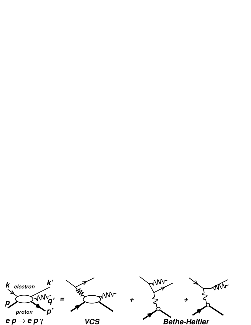
Figure 1: Lowest order QED diagrams for the process $ep\rightarrow ep\gamma$, including the DVCS and Bethe-Heitler (BH) amplitudes. The external momentum four-vectors are defined on the diagram. The virtual photon momenta are $q^{\mu}=(k-k^{\prime})^{\mu}$ in the DVCS- and $\Delta^{\mu}=(q-q^{\prime})^{\mu}$ in the BH-amplitudes.

The factorization proofs Ji and Osborne (1998); Collins and Freund (1999) established that the GPDs are experimentally accessible through deeply virtual Compton scattering (DVCS) and its interference with the Bethe-Heitler (BH) process (Fig. 1). In addition, the spatial resolution ($Q^{2}$) of the reaction is independent of the distance scale $\approx 1/\sqrt{t_{\rm min}-t}$ probed. Quark-Gluon operators are classified by their twist: the dimension minus spin of each operator. The handbag amplitude of Fig. 2 is the lowest twist (twist-2) $\gamma^{\ast}p\rightarrow\gamma p$ operator. The factorization proofs confirm the connection between DIS and DVCS. The proofs therefore suggest (but do not establish) that, just as in DIS, higher twist terms in DVCS will be only a small contribution to the cross sections at the $Q^{2}$ and $x_{\rm Bj}$ range accessible with electrons from 6–12 GeV.

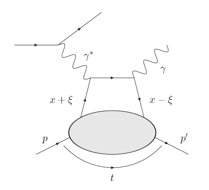
Figure 2: Leading twist $\gamma^{\ast}p\rightarrow\gamma p$ amplitude in the DVCS limit. The initial and final quarks carry light-cone momentum fractions $x+\xi$ and $x-\xi$ of the light-cone momenta $(1\pm\xi)(p+p^{\prime})^{+}$ (Eq. 7). The crossed diagram is also included in the full DVCS amplitude. The invariant momentum transfer squared to the proton is $t=\Delta^{2}$.

In the formalism we are using Belitsky et al. (2002), the matrix elements of operators of twist-$n$ are $Q^{2}$ independent (except for $\ln(Q^{2}/\Lambda_{\rm QCD}^{2})$ evolution), but all observables of twist-$n$ operators carry kinematic pre-factors that scale as $[(t_{\rm min}-t)/Q^{2}]^{n/2}$, $[(-t)/Q^{2}]^{n/2}$, or $[M^{2}/Q^{2}]^{n/2}$. Diehl et al., Diehl et al. (1997) showed that the twist-2 and twist-3 DVCS-BH interference terms could be independently extracted from the azimuthal-dependence ($\phi_{\gamma\gamma}$, §II.1) of the helicity dependent cross sections. Burkardt Burkardt (2000) showed that the $t$-dependence of the GPDs at $\xi=0$ is Fourier conjugate to the transverse spatial distribution of quarks in the infinite momentum frame as a function of momentum fraction. Ralston and Pire Ralston and Pire (2002) and Diehl Diehl (2002) extended this interpretation to the general case of $\xi\neq 0$. Belitsky et al., Belitsky et al. (2004) describe the general GPDs in terms of quark and gluon Wigner functions.

These elegant theoretical concepts have stimulated an intense experimental effort in DVCS. The H1 Aktas et al. (2005) Adloff et al. (2001) and ZEUS Chekanov et al. (2003) collaborations at HERA measured cross sections for $x_{\rm Bj}\approx 2\xi\approx 10^{-3}$. These data are integrated over $\phi_{\gamma\gamma}$ and are therefore not sensitive to the BH$\cdot$DVCS interference terms. The CLAS Stepanyan et al. (2001) and HERMES Airapetian et al. (2001) collaborations measured relative beam helicity asymmetries. HERMES has also measured relative beam charge asymmetries Ellinghaus (2002); Airapetian et al. (2006) and CLAS has measured longitudinal target relative asymmetries Chen et al. (2006). The HERA and HERMES results integrate over final state inelasticities of $M_{X}^{2}\leq 2.9\,{\rm GeV}^{2}$ (or greater). Relative asymmetries are a ratio of cross section differences divided by a cross section sum. In general, these relative asymmetries contain BH$\cdot$DVCS interference and DVCS^†DVCS terms in both the numerator and denominator (the beam charge asymmetry removes the DVCS^†DVCS terms only from the numerator). Absolute cross section measurements are necessary to obtain all DVCS observables.

In Hall A, E00-110Roblin et al. (2000) and E03-106Voutier et al. (2003), we measured absolute cross sections for H$(\vec{e},e^{\prime}\gamma)$p and D$(e,e^{\prime}\gamma)pn$ at $x_{\rm Bj}=0.36$. The following section describes the methods and results of E00-110. We propose to continue this program using the same experimental techniques, while taking advantage of the higher beam energy available with CEBAF at 12 GeV.

I.2 Review of Hall A DVCS E00-110 Methods and Results

The first draft publication of E00-110 can be found in Ref. Muñoz Camacho et al. (2006). Using a well understood experimental apparatus, this experiment measured both the unpolarized and polarized cross-section of the $\vec{e}p\rightarrow ep\gamma$ process in the Deeply Virtual Compton Scattering (DVCS) regime at $x_{\rm Bj}=0.36$ and for Q² at 1.5, 1.9, and 2.3 GeV² . With electrons detected in the HRS-L, we have an absolute acceptance for electron detection understood to 3%, and a precise measurement of the scattering vertex and the direction of the virtual photon. DVCS is a three body final state, but at high $Q^{2}$ and low $t$, the final photon is highly aligned with the virtual photon and therefore highly correlated with the scattered electron. Thus, even with a modest calorimeter, our coincidence acceptance for DVCS is essentially limited only by the electron spectrometer. As a consequence, very high values of the product of luminosity times coincidence acceptance are possible. The radiation hard PbF₂ calorimeter gives a fast (Cerenkov) time response, and each channel is recorded with a 1 GHz digitizer which allows off-line identification of the DVCS photon. The identification of the exclusive channel is illustrated in Fig. 3. In Hall A, our systematic errors are minimized by the combination of the Compton polarimeter, the well-understood optics and acceptance of the High Resolution Spectrometer (HRS), and a compact, hermetic, calorimeter. All of those factors allowed the measurements of cross-sections. The high-precision electron detection minimizes systematic errors on $t$ and $\phi_{\gamma\gamma}$. Therefore, we exploit the precision $\phi_{\gamma\gamma}$-dependence to extract the cross section terms which have the form of a finite Fourier series modulated by the electron propagators of the BH amplitude.

The strong point of experiment E00-100 is that we measured absolute cross-sections. For example, the $\sin(\phi)$ term (modulated by BH propagators) of the helicity dependent cross section measures the interference of the imaginary part of the twist-2 DVCS amplitude with the BH amplitude, with a small contribution from an additional twist-3 bilinear DVCS term. The $Q^{2}$-dependence of this term places a tight limit on the contribution of the higher twist terms to our extraction of the “handbag” amplitude. The unpolarized cross section is a sum of the BH cross section, the real part of the BH$\cdot$DVCS interference, and a twist-2 bilinear DVCS term. The E00-110 results show that the unpolarized cross section is not entirely dominated by the BH cross section, but also has a large contribution from DVCS. Explicit twist-3 terms were also extracted from the $\sin(2\phi_{\gamma\gamma})$ and $\cos(2\phi_{\gamma\gamma})$ dependence of the cross sections. These contribute very little to the cross sections.

In the kinematic regime of E00-100, neither the extracted Twist-2 or Twist-3 observables show any statistically significant dependence on Q² . This provides strong support to the original theoretical predictions that DVCS scaling is based on the same foundation as DIS scaling. We note that in the range $0.2\leq x_{\rm Bj}\leq 0.6$, both the higher twist terms and $\ln Q^{2}/\Lambda_{QCD}^{2}$ evolution terms are small in DIS, even for $\mbox{Q${}^{2}$ }\approx 2$ GeV² Schaefer et al. (2001); Osipenko et al. (2005); Eidelman et al. (2004). Thus we are well on our way to proving the dominance of the leading twist term of the amplitudes ( “handbag approximation”) where the virtual photon scatters off a single parton. This approximation is a corner stone of the study of the nucleon structure in terms of GPDs.

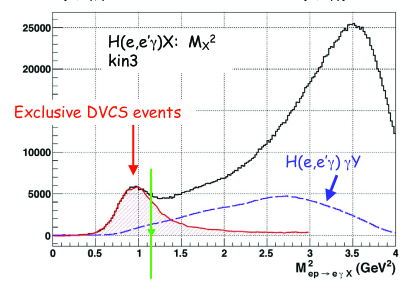
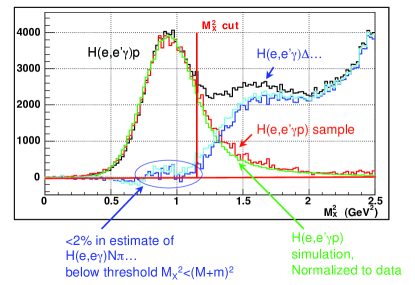
Figure 3: Missing mass squared distribution for the H$(e,e^{\prime}\gamma)X$ reaction, obtained in Hall A in E00-110. The left plot shows the raw spectrum (after accidental subtraction) and the statistical estimate of the contribution of $ep\rightarrow eY\pi^{0}$ events of the type H$(e,e^{\prime}\gamma)\gamma Y$. This estimate was obtained from the ensemble of detected H$(e,e^{\prime}\pi^{0})Y$ events, with both photons from the $\pi^{0}\rightarrow\gamma\gamma$ decay detected in the calorimeter. The right plot shows the H$(e,e^{\prime}\gamma)X$ spectrum, after the $\pi^{0}$ subtraction.

I.3 Physics Goals and Proposed DVCS Kinematics

The present proposal cannot fully disentangle the spin-flavor structure of the GPDs. We itemize here the measurements we will perform and the physical insights we expect to obtain.

• Measure the $\vec{e}p\rightarrow ep\gamma$ cross sections at fixed $x_{\rm Bj}$ over as wide a range in $Q^{2}$ as possible for $k\leq 11$ GeV. This will determine with what precision the handbag amplitude dominates (or not) over the higher twist amplitudes. More generally, we consider the virtual photon at high $Q^{2}$ as a superposition of a point-like elementary photon and a ‘hadronic’ photon ($q\overline{q}$, vector mesons) with a typical hadronic transverse size. The $Q^{2}$ dependence of the DVCS cross sections measures the relative importance of these two components of the photon Bauer et al. (1978).

• Extract all kinematically independent observables (unpolarized target) for each $Q^{2}$, $x_{\rm Bj}$, $t$ point. These observables are the angular harmonic superposition of Compton Form Factors (CFFs). As functions of $\phi_{\gamma\gamma}$, the observable terms are $\cos(n\phi_{\gamma\gamma})$ for $n\in\{0,1,2\}$, and $\sin(n\phi_{\gamma\gamma})$ for $n\in\{1,2\}$, with additional $1/[J+K\cos(\phi_{\gamma\gamma})]$ modulations from the electron propagators of the BH amplitude (§II.2). Each of these five observables isolates the $\Re\text{e}$ or $\Im\text{m}$ parts of a distinct combination of linear ($BH\cdot DVCS^{\dagger}$) and bilinear ($DVCS\cdot DVCS^{\dagger}$) terms.

• Measure the $t$-dependence of each angular harmonic term. The $t$-dependence of each CFF is Fourier-conjugate to the spatial distribution of the corresponding superposition of quark distributions in the nucleon, as a function of quark light-cone momentum-fraction. In a single experiment, we cannot access this Fourier transform directly, because we measure a superposition of terms. However, we still expect to observe changes in the $t$-dependence of our observables as a function of $x_{\rm Bj}$. In particular, the $r.m.s.$ impact parameter of a quark of momentum fraction $x$ must diminish as a power of $(1-x)$ as $x\rightarrow 1$. This is not a small effect, between $x=0.36$ and $x=0.6$, we expect a change in slope (as a function of $t$) of a factor two in individual GPDs.

• Measure the $\vec{e}p\rightarrow ep\pi^{0}$ cross section in the same kinematics as DVCS.
  This will test the factorization dominance of meson electro-production. The longitudinal cross section ($d^{2}\sigma_{L}$) is the only leading twist (twist-2) term in the electro-production cross section. In this experiment, we do not propose Rosenbluth separations of $d^{2}\sigma_{L}$ from $d^{2}\sigma_{T}$. However, as a function of $Q^{2}$, the ratio $d^{2}\sigma_{T}/d^{2}\sigma_{L}$ falls at least $\propto 1/Q^{2}$. Thus the handbag contribution to $d^{2}\sigma_{L}$ can be extracted, within statistical errors, from a $1/Q^{2}$ expansion. The $\sigma_{LT}$, $\sigma_{TT}$, and $\sigma_{LT^{\prime}}$ terms will be obtained from a Fourier decomposition of the azimuthal dependence of the cross section. These observables will provide additional constraints on both the longitudinal and transverse currents in pion electro-production.
  The handbag amplitude of pion electro-production is the convolution of the axial GPDs $\tilde{H}$ and $\tilde{E}$ with the pion distribution amplitude (DA) $\Phi_{\pi}$. For charged pion electro-production, the $\tilde{E}$ term is expected to be dominated by the pion-pole–this is the mechanism used to measure the pion form factor in electro-production on the proton. However, neutral pion electro-production will be dominated by the non-pion-pole contributions to $\tilde{H}$ and $\tilde{E}$.

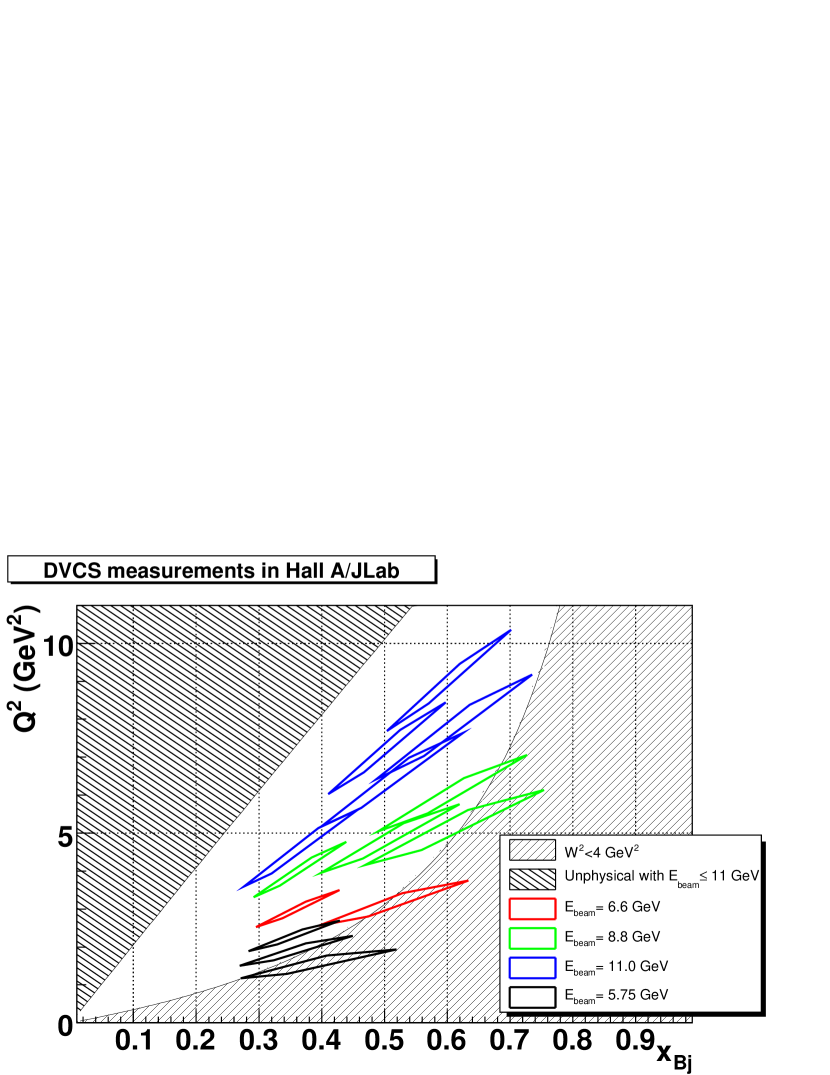
Figure 4: Proposed DVCS kinematics for H$(e,e^{\prime}\gamma)p$ measurements in Hall A with 3, 4, and 5 pass beams of CEBAF at 12 GeV. The diamond shapes trace the approximate acceptance of the HRS in each setting. The boundary of the unphysical region corresponds to the maximum possible $Q^{2}$ at a given $x_{\rm Bj}$ for 11 GeV. This corresponds to $180^{\circ}$ electron scattering, equivalent to $\theta_{q}=0^{\circ}$. The points at $E_{\text{B}eam}=5.75$ GeV were obtained in E00-110.

To study the DVCS process with CEBAF at 12 GeV, we limit our definition of DVCS to the following kinematic range for the central values of our Hall A configurations:

$$Q^{2} \geq 2\,{\rm GeV}^{2}$$

$$W^{2} \geq 4\,{\rm GeV}^{2}$$

$$-t < Q^{2}$$ (1)

Our proposed kinematics, and the physics constraints of Eq. I.3 are illustrated in Fig. 4. We propose a $Q^{2}$ scan of the cross sections for three values of $x_{B}$. Our maximum central $Q^{2}$ of 9 GeV² is higher than the $Q^{2}$ range of the $t$-distributions of published DVCS cross sections (integrated over $\phi_{\gamma\gamma}$) from HERA for $x_{\rm Bj}\approx 10^{-3}$. The beam time estimates for these high statistics measurements are listed in Table 1.

Within the experimental constraints which we detail in section III, our choice of kinematics responds to the physics goals of high beam energy DVCS measurements.

• At each $x_{\rm Bj}$ point, we measure the maximum possible range in $Q^{2}$. Although our preliminary data from E00-110 at $x_{\rm Bj}=0.36$ show no indication of $Q^{2}$ dependence in the observable $\Im\text{m}[{\mathcal{C}}^{\mathcal{I}}(\mathcal{F})]$, this could result from a compensation of terms of higher twist and QCD evolution. In this proposal, we will double the range in $Q^{2}$ at $x_{\rm Bj}=0.36$, and provide a nearly equal $Q^{2}$ range at $x_{\rm Bj}=0.5$ and $0.6$.

• Simple kinematics dictates that as the momentum fraction $x+\xi$ of the struck quark goes to 1, its impact parameter $b/(1+\xi)$ relative to the center of momentum of the initial proton must shrink towards zero. Burkardt has discussed the “shrinkage” of the proton as $x\rightarrow 1$ in the limit $\xi=0$. Burkardt (2004); Burkardt and Miller (2003). The perpendicular momentum transfer $\Delta_{\perp}$ is Fourier conjugate to the impact parameter $b$. As a function of $x$, the mean square transverse separation between the struck quark and the center-of-momentum of the spectator system is

  $$\langle{\bf r}_{\perp}^{2}\rangle(x)=\langle b^{2}\rangle/(1-x)^{2},$$ (2)

  where $\langle b^{2}\rangle$ is the mean square impact parameter of the struck quark. Burkardt considered GPD models of the form

  $$H_{f}(x,0,t)=q_{f}(x)\exp\left[at(1-x)^{n}/x\right].$$ (3)

  The bound that $\langle{\bf r}_{\perp}^{2}\rangle$ remain finite as $x\rightarrow 1$ requires $n\geq 2$. On the other hand, $n=1$ has been used extensively for modeling GPDs. At $x=0.6$, the choice of $n=1$ or $n=2$ changes the logarithmic slope $\partial\ln H/\partial t$ by a factor 2.5. This model illustrates that without measurements, there are very large uncertainties in the behavior of the GPDs at large $x$ (independent of the $t=0$ constraints), and that measurements will improve our understanding of the transverse distance scales of the quarks and gluons inside the proton.

Our specific choice of kinematics in Fig. 4 and Table 1 maximizes our range in $x_{\rm Bj}$, while maintaining measurements as a function of $Q^{2}$ for each value of $x_{\rm Bj}$.

$Q^{2}$	$k$	Beam Time			Total (Days)
(GeV2)	(GeV)	$\ x_{\rm Bj}=0.36\$	$\ x_{\rm Bj}=0.50\$	$\ x_{\rm Bj}=0.6\$	(Days)
3.0	6.6	3
4.0	8.8	2
4.55	11.0	1
3.1	6.6		5
4.8	8.8		4
6.3	11.0		4
7.2	11.0		7
5.1	8.8			13
6.0	8.8			16
7.7	11.0			13
9.0	11.0			20
TOTAL		6	20	62	88

Table 1: Proposed Beam Time as a function of $(Q^{2},k,x_{\rm Bj})$ DVCS kinematics.

II DVCS Observables

II.1 DVCS Kinematics and Definitions

Fig. 1 defines our kinematic four-vectors for the $ep\rightarrow ep\gamma$ reaction. The cross section is a function of the following invariants defined by the electron scattering kinematics:

$$s_{e} = (k+p)^{2}=M^{2}+2kM$$

$$Q^{2} = -q^{2}$$

$$W^{2} = (q+p)^{2}=M^{2}+Q^{2}\left[{1\over x_{\rm Bj}}-1\right]$$

$$x_{\rm Bj} = {Q^{2}\over 2q\cdot p}={Q^{2}\over W^{2}-M^{2}+Q^{2}}$$

$$y = q\cdot p/k\cdot p.$$ (4)

The DVCS cross section also depends on variables specific to deeply virtual electro-production: the DVCS scaling variable $\xi$, the invariant momentum transfer squared $t$ to the proton,azimuth $\phi_{\gamma\gamma}$ of the final photon around the ${\bf q}$-vector direction. The DVCS scaling variable $\xi$ is defined in terms of the symmetrized momenta:

$$\xi = {-\overline{q}^{2}\over\overline{q}\cdot P}$$ (5)

$$= x_{\rm Bj}{1+t/Q^{2}\over 2-x_{\rm Bj}(1-t/Q^{2})}$$

$$\rightarrow{x_{\rm Bj}\over 2-x_{\rm Bj}}\ \ {\rm for}\ |t|/Q^{2}<<1$$

$$\overline{q}^{\mu} = (q+q^{\prime})^{\mu}/2$$

$$P^{\mu} = (p+p^{\prime})^{\mu}.$$

$$P^{2} = 4M^{2}-t$$

$$t = (p^{\prime}-p)^{2}=\Delta^{2}.$$ (6)

In light cone coordinates $(p^{+},{\bf p}_{\perp},p^{-})$, with $p^{\pm}=(p^{0}\pm p^{z})/\sqrt{2}$, the four-vectors are:

$$p = \left[(1+\xi)P^{+},\frac{-\Delta_{\perp}}{2},\frac{M^{2}+\Delta_{\perp}^{2}/4}{2P^{+}(1+\xi)}\right]$$

$$p^{\prime} = \left[(1-\xi)P^{+},\frac{+\Delta_{\perp}}{2},\frac{M^{2}+\Delta_{\perp}^{2}/4}{2P^{+}(1-\xi)}\right]$$

$$P = \left[P^{+},0,\frac{4M^{2}-t}{2P^{+}}\right].$$ (7)

In Fig. 1, the initial (final) quark light cone momentum fraction is $x\pm\xi$ of the symmetrized momentum $P$ and $(x\pm\xi)/(1\pm\xi)$ of the initial (final) proton momentum $p^{+}$ ($p^{\prime\,+}$).

Our convention for $\phi_{\gamma\gamma}$ is defined as the azimuthal angle in a event-by-event spherical-polar coordinate system (in the lab):

$$\hat{z}_{q} = {\bf q}/|{\bf q}|$$

$$\hat{y}_{q} = \left[{\bf k}\times{\bf k}^{\prime}\right]/|{\bf k}\times{\bf k}^{\prime}|$$

$$\hat{x}_{q} = \hat{y}_{q}\times\hat{z}_{q}.$$ (8)

$$\tan(\phi_{\gamma\gamma}) = \left.({\bf q}^{\prime}\cdot\hat{y}_{q})\right/({\bf q}^{\prime}\cdot\hat{x}_{q})$$ (9)

$$= \left.\left[|{\bf q}|{\bf q}^{\prime}\cdot({\bf k}\times{\bf k}^{\prime}\right]\right/\left[{\bf q}\times{\bf q}^{\prime})\cdot({\bf k}\times{\bf k}^{\prime})\right].$$

The quadrant of $\phi_{\gamma\gamma}$ is defined by the signs of $({\bf q}^{\prime}\cdot\hat{y}_{q})$ and $({\bf q}^{\prime}\cdot\hat{x}_{q})$ We also utilize the laboratory angle $\theta_{\gamma\gamma}$ between the ${\bf q}$-vector and ${\bf q}^{\prime}$-directions:

$$\cos\theta_{\gamma\gamma} = \hat{z}_{q}\cdot{\bf q^{\prime}}/|{\bf q^{\prime}}|.$$ (10)

The impact parameter $b$ of the light-cone matrix element is Fourier conjugate to the $\Delta_{\perp}$, the momentum transfer perpendicular to the light cone direction defined by $P^{+}$:

$$\Delta^{2}_{\perp} = (t-t_{\rm min})\frac{(1-\xi^{2})}{(1+\xi^{2})}$$ (11)

$$t_{\rm min}=t(\theta_{\gamma\gamma}=0^{\circ}) = \frac{-4M^{2}\xi^{2}}{1-\xi^{2}}\approx\frac{-x_{\rm Bj}^{2}M^{2}}{\left[1-x_{\rm Bj}(1-M^{2}/Q^{2})\right]}.$$ (12)

II.2 DVCS Cross Section

The following equations reproduce the consistent expansion of the DVCS cross section to order twist-3 of Belitsky, Müller, and Kirchner Belitsky et al. (2002). Note that our definition of $\phi_{\gamma\gamma}$ agrees with the “Trento-Convention” for $\phi$ Bacchetta et al. (2004), and is the definition used in Airapetian et al. (2001) and Stepanyan et al. (2001). Note also that this azimuth convention differs from $\phi_{\text{\cite[cite]{\@@bibref{Authors Phrase1YearPhrase2}{Belitsky:2001ns}{\@@citephrase{(}}{\@@citephrase{)}}}}}$ defined in Belitsky et al. (2002) by $\phi_{\gamma\gamma}=\pi-\phi_{\text{\cite[cite]{\@@bibref{Authors Phrase1YearPhrase2}{Belitsky:2001ns}{\@@citephrase{(}}{\@@citephrase{)}}}}}$. In the following expressions, we utilize the differential phase space element $d^{5}\Phi=dQ^{2}dx_{\rm Bj}d\phi_{e}dtd\phi_{\gamma\gamma}$. The helicity-dependent ($\lambda=\pm 1$) cross section for a lepton of charge $\pm e$ on an unpolarized target is:

$$\frac{d^{5}\sigma(\lambda,\pm e)}{d^{5}\Phi} = \frac{d\sigma_{0}}{dQ^{2}dx_{\rm Bj}}\left|\mathcal{T}^{BH}(\lambda)\pm\mathcal{T}^{DVCS}(\lambda)\right|^{2}/|e|^{6}$$ (13)

$$= \frac{d\sigma_{0}}{dQ^{2}dx_{\rm Bj}}\left[\left|\mathcal{T}^{BH}(\lambda)\right|^{2}+\left|\mathcal{T}^{DVCS}(\lambda)\right|^{2}\mp\mathcal{I}(\lambda)\right]\frac{1}{e^{6}}$$

$$\frac{d\sigma_{0}}{dQ^{2}dx_{\rm Bj}} = \frac{\alpha_{\rm QED}^{3}}{16\pi^{2}(s_{e}-M^{2})^{2}x_{\rm Bj}}\frac{1}{\sqrt{1+\epsilon^{2}}}$$

$$\epsilon^{2} = 4M^{2}x_{\rm Bj}^{2}/Q^{2}$$ (14)

The $|\mathcal{T}^{BH}|^{2}$ term is given in Belitsky et al. (2002), Eq. 25, and will not be reproduced here, except to note that it depends on bilinear combinations of the ordinary elastic form factors $F_{1}(t)$ and $F_{2}(t)$. The interference term $\mathcal{I}$ is:

$$\frac{1}{e^{6}}\mathcal{I} = \frac{1}{x_{\rm Bj}y^{3}\mathcal{P}_{1}(\phi_{\gamma\gamma})\mathcal{P}_{2}(\phi_{\gamma\gamma})t}\left\{c_{0}^{\mathcal{I}}+\sum_{n=1}^{3}(-1)^{n}\left[c_{n}^{\mathcal{I}}(\lambda)\cos(n\phi_{\gamma\gamma})-\lambda s_{n}^{\mathcal{I}}\sin(n\phi_{\gamma\gamma})\right]\right\}.$$ (15)

The $(-1)^{n}$ and $(-\lambda)$ factors are introduced by our convention for $\phi_{\gamma\gamma}$, relative to Belitsky et al. (2002). The bilinear DVCS terms have a similar form:

$$\left|\mathcal{T}^{DVCS}(\lambda)\right|^{2}\frac{1}{e^{6}} = \frac{1}{y^{2}Q^{2}}\left\{c_{0}^{DVCS}+\sum_{n=1}^{2}(-1)^{n}c_{n}^{DVCS}\cos(n\phi_{\gamma\gamma})+\lambda s_{1}^{DVCS}\sin(\phi_{\gamma\gamma})\right\}$$ (16)

The Fourier coefficients $c_{n}$ and $s_{n}$ will be defined below (Eq. 21–27). The $c_{n}^{\mathcal{I}}$ and $s_{n}^{\mathcal{I}}$ are linear in the GPDs, the $c_{n}^{\mathcal{D}VCS}$ and $s_{n}^{\mathcal{D}VCS}$ are bi-linear in the GPDs (and their higher twist extensions). All of the $\phi_{\gamma\gamma}$-dependence of the cross section is now explicit in Eq. 15 and 16.

The $\mathcal{P}_{i}(\phi_{\gamma\gamma})$ are the electron propagators of the BH amplitude:

$$Q^{2}\mathcal{P}_{1}(\phi_{\gamma\gamma}) = (k-q^{\prime})^{2}$$

$$Q^{2}\mathcal{P}_{2}(\phi_{\gamma\gamma}) = (k^{\prime}+q^{\prime})^{2}.$$ (17)

After some algebra, the kinematic dependence of the pre-factor of Eq. 15 is more apparent:

$$\frac{1}{x_{\rm Bj}y^{3}\mathcal{P}_{1}(\phi_{\gamma\gamma})\mathcal{P}_{2}(\phi_{\gamma\gamma})t} = \frac{-(1+\epsilon^{2})^{2}(s_{e}-M^{2})/t}{Q^{2}\left(J-2K\cos\phi_{\gamma\gamma}\right)\left(1+J+(t/Q^{2})-2K\cos\phi_{\gamma\gamma}\right)}$$ (18)

$$J = \left[1-y-\frac{y\epsilon^{2}}{2}\right]\left(1+\frac{t}{Q^{2}}\right)+\left(1-x_{\rm Bj}\right)\left(2-y\right)\left(\frac{-t}{Q^{2}}\right)$$ (19)

$$\rightarrow\left[1-y-\frac{y\epsilon^{2}}{2}\right]\ \ {\rm as}\ t/Q^{2}\rightarrow 0$$

$$K^{2} = \frac{t_{\rm min}-t}{Q^{2}}\left(1-x_{\rm Bj}\right)\left[1-y-\frac{y^{2}\epsilon^{2}}{4}\right]\left[\sqrt{1+\epsilon^{2}}-\frac{x_{\rm Bj}W^{2}}{W^{2}-M^{2}}\frac{(t_{\rm min}-t)}{Q^{2}}\right]$$ (20)

$$\rightarrow\frac{t_{\rm min}-t}{Q^{2}}\left(1-x_{\rm Bj}\right)\left[1-y\right]\ \ {\rm as}\ t/Q^{2}\rightarrow 0$$

The coefficient $K$ appears not only in the BH propagators, but also in the kinematic prefactors of the Fourier decomposition of the cross section (see below). For fixed $Q^{2}$ and $x_{\rm Bj}$, $K$ depends on $t$ as $(t_{\rm min}-t)/Q^{2}$.

II.3 Fourier Coefficients and Angular Harmonics

The Fourier coefficients $c^{\mathcal{I}}_{n}$ and $s^{\mathcal{I}}_{n}$ of the interference terms are:

$$c_{0}^{\mathcal{I}} = -8(2-y)\Re\text{e}\left\{\frac{(2-y)^{2}}{1-y}K^{2}\mathcal{C}^{\mathcal{I}}(\mathcal{F})+\frac{t}{Q^{2}}(1-y)(1-x_{\rm Bj})\left[\mathcal{C}^{\mathcal{I}}+\Delta\mathcal{C}^{\mathcal{I}}\right](\mathcal{F})\right\}$$

$$\left\{{c_{1}^{\mathcal{I}}\atop\lambda s_{1}^{\mathcal{I}}}\right\} = -8K\left\{{(2-2y+y^{2})\atop-\lambda y(2-y)}\right\}\left\{{\Re\text{e}\atop\Im\text{m}}\right\}\mathcal{C}^{\mathcal{I}}(\mathcal{F})$$

$$\left\{{c_{2}^{\mathcal{I}}\atop\lambda s_{2}^{\mathcal{I}}}\right\} = \frac{-16K^{2}}{2-x_{\rm Bj}}\left\{{(2-y)\atop-\lambda y}\right\}\left\{{\Re\text{e}\atop\Im\text{m}}\right\}\mathcal{C}^{\mathcal{I}}(\mathcal{F}^{\rm eff})$$ (21)

The Fourier coefficients $c_{3}^{\mathcal{I}}$, $s_{3}^{\mathcal{I}}$ are gluon transversity terms. We expect these to be very small in our kinematics, though it would be exciting if they generated a measureable signal. The ${\mathcal{C}^{I}}$ and $\Delta{\mathcal{C}^{I}}$ amplitudes are the angular harmonic terms defined in Eqs. 69 and 72 of Belitsky et al. (2002) (we have suppressed the subscript “unp” since our measurements are only with an unpolarized target). These angular harmonics depend on the interference of the BH amplitude with the set ${\mathcal{F}}=\{{\mathcal{H},\,\mathcal{E},\,\tilde{\mathcal{H}},\,\tilde{\mathcal{E}}}\}$ of twist-2 Compton form factors (CFFs) or the related set ${\mathcal{F}}^{\rm eff}$ of effective twist-3 CFFs:

$${\mathcal{C}^{I}}({\mathcal{F}}) = F_{1}(t){\mathcal{H}}(\xi,t)+\xi G_{M}(t)\tilde{\mathcal{H}}(\xi,t)-{t\over 4M^{2}}F_{2}(t){\mathcal{E}}(\xi,t)$$ (22)

$${\mathcal{C}^{I}}({\mathcal{F}}^{\rm eff}) = F_{1}(t){\mathcal{H}}^{\rm eff}(\xi,t)+\xi G_{M}(t)\tilde{\mathcal{H}}^{\rm eff}(\xi,t)-{t\over 4M^{2}}F_{2}(t){\mathcal{E}}^{\rm eff}(\xi,t)$$ (23)

$$\left[{\mathcal{C}^{I}}+\Delta{\mathcal{C}^{I}}\right]({\mathcal{F}}) = F_{1}(t){\mathcal{H}}(\xi,t)-{t\over 4M^{2}}F_{2}(t){\mathcal{E}}(\xi,t)-\xi^{2}G_{M}(t)\left[{\mathcal{H}}(\xi,t)+{\mathcal{E}}(\xi,t)\right].$$ (24)

Note that $\left[{\mathcal{C}^{I}}+\Delta{\mathcal{C}^{I}}\right]$ depends only on ${\mathcal{H}}$ and ${\mathcal{E}}$. The usual proton elastic form factors, $F_{1}$, $F_{2}$ and $G_{M}=F_{1}+F_{2}$ are defined to have negative arguments in the space-like regime. The Compton form factors are defined in terms of the vector GPDs $H$ and $E$, and the axial vector GPDs $\tilde{H}$ and $\tilde{E}$. For example ($f\in\{u,d,s\}$) Belitsky et al. (2002):

$${\mathcal{H}}(\xi,t) = \sum_{f}\left[\frac{e_{f}}{e}\right]^{2}\Biggl{\{}i\pi\left[H_{f}(\xi,\xi,t)-H_{f}(-\xi,\xi,t)\right]$$ (25)

$$+{\mathcal{P}}\int_{-1}^{+1}dx\left[\frac{1}{\xi-x}-\frac{1}{\xi+x}\right]H_{f}(x,\xi,t)\Biggr{\}}.$$

Twist-3 CFFs contain Wandzura-Wilzcek terms, determined by the twist-2 matrix elements, and dynamic $qGq$ twist-3 matrix elements. The twist-2 and twist-3 CFFs are matrix elements of quark-gluon operators and are independent of $Q^{2}$ (up to logarithmic QCD evolution). The kinematic suppression of the twist-3 (and higher) terms is expressed in powers of $-t/Q^{2}$ and $(t_{\rm min}-t)/Q^{2}$ in e.g. the $K$-factor. This kinematic suppression is also a consequence of the fact that the the twist-3 terms couple to the longitudinal polarization of the virtual photon.

The bilinear DVCS Fourier coefficients are:

$$c_{0}^{\text{D}VCS} = 2(2-2y+y^{2})\mathcal{C}^{\text{D}VCS}(\mathcal{F},\mathcal{F}^{\ast})$$

$$\begin{Bmatrix}{c_{1}^{\text{D}VCS}}\\ {\lambda s_{1}^{\text{D}VCS}}\end{Bmatrix} = \frac{8K}{2-x_{\rm Bj}}\begin{Bmatrix}2-y\\ -\lambda y\end{Bmatrix}\begin{Bmatrix}\Re\text{e}\\ \Im\text{m}\end{Bmatrix}\mathcal{C}^{\text{D}VCS}(\mathcal{F}^{\text{e}ff},\mathcal{F}^{\ast})$$ (26)

The $c_{2}^{\text{D}VCS}$ coefficient is a gluon transversity term.

The DVCS angular harmonics are

$$\mathcal{C}^{DVCS}(\mathcal{F},\mathcal{F}^{\ast}) = \frac{1}{(2-x_{\rm Bj})^{2}}\left\{4(1-x_{\rm Bj})\left(\mathcal{H}\mathcal{H}^{\ast}+\tilde{\mathcal{H}}\tilde{\mathcal{H}}^{\ast}\right)-x_{\rm Bj}^{2}2\Re\text{e}\left[\mathcal{H}\mathcal{E}^{\ast}+\tilde{\mathcal{H}}\tilde{\mathcal{E}}^{\ast}\right]\right.$$ (27)

$$\left.-\left(x_{\rm Bj}^{2}+(2-x_{\rm Bj})^{2}\frac{t}{4M^{2}}\right)\mathcal{E}\mathcal{E}^{\ast}-x_{\rm Bj}^{2}\frac{t}{4M^{2}}\tilde{\mathcal{E}}\tilde{\mathcal{E}}^{\ast}\right\}.$$

The twist-3 term $\mathcal{C}^{DVCS}(\mathcal{F}^{\rm eff},\mathcal{F}^{\ast})$ has an identical form, with one CFF factor replaced with the set $\mathcal{F}^{\rm eff}$. The $\mathcal{C}^{DVCS}(\mathcal{F}_{T},\mathcal{F}^{\ast})$, appearing with a $\cos(2\phi_{\gamma\gamma})$ weighting, also has the same form as Eq. 27, but now with one set $\mathcal{F}$ replaced by the set $\mathcal{F}_{T}$ of (twist-2) gluon transversity Compton form factors.

II.4 BH$\cdot$DVCS Interference and Bilinear DVCS Terms

The BH$\cdot$DVCS interference terms are not fully separable from the bilinear DVCS terms. We analyze the cross section (e.g. Muñoz Camacho et al. (2006)) in the general form

$$\frac{d^{5}\sigma}{d^{5}\Phi} = \frac{d^{5}\sigma^{BH}}{d^{5}\Phi}+\frac{1}{\mathcal{P}_{1}(\phi_{\gamma\gamma})\mathcal{P}_{2}(\phi_{\gamma\gamma})}\sum_{n}\left\{K_{cn}\Re\text{e}\left[\mathcal{C}_{n}^{\mathcal{I},\rm exp}\right]\cos(n\phi_{\gamma\gamma})\right.$$ (28)

$$\left.+\lambda K_{sn}\Im\left[\mathcal{C}_{n}^{\mathcal{I},\rm exp}\right]\sin(n\phi_{\gamma\gamma})\right\}$$

The factors $K_{cn,sn}$ are the purely kinematic pre-factors defined in Eqs. 13–21. The experimental coefficients $\Re\text{e},\Im\text{m}\mathcal{C}_{n}^{\mathcal{I},\rm exp}$ include contributions from the bilinear DVCS terms, that mix into different orders in $\cos(n\phi)$ or $\sin(n\phi)$ due to the absence of the BH propagators $\mathcal{P}_{1}\mathcal{P}_{2}$ in the DVCS² cross section.

From Eq. 18, 15, and 16, we obtain the generic enhancement of the interference terms over the DVCS^†DVCS terms (of the same order in $\sin(n\phi_{\gamma\gamma})$ or $\cos(n\phi_{\gamma\gamma})$):

$$\left|\frac{BH\cdot DVCS}{DVCS^{\dagger}DVCS}\right| \propto \frac{y^{2}(s_{e}-M^{2})}{-t}.$$ (29)

In each setting $(x_{\rm Bj},Q^{2})$ setting, for each bin in $t$, we therefore have the following experimental Twist-2 DVCS observables

$$\Im\text{m}[\mathcal{C}^{\mathcal{I},\rm exp}(\mathcal{F})] = \Im\text{m}[\mathcal{C}^{\mathcal{I}}(\mathcal{F})]+\langle\eta_{s1}\rangle\Im\text{m}[\mathcal{C}^{DVCS}(\mathcal{F}^{\ast},\mathcal{F}^{\rm eff})]$$ (30)

$$\Re\text{e}\left\{[\mathcal{C}+\Delta\mathcal{C}]^{\mathcal{I},\rm exp}(\mathcal{F})\right\} = \Re\text{e}\left\{[\mathcal{C}^{\mathcal{I}}+\Delta\mathcal{C}^{\mathcal{I}}](\mathcal{F})\right\}+\langle\eta_{0}\rangle\,\Re\text{e}\left[\mathcal{C}^{\rm DVCS}(\mathcal{F}^{\ast},\mathcal{F})\right]$$ (31)

$$\Re\text{e}\left\{\mathcal{C}^{\mathcal{I},\rm exp}(\mathcal{F})\right\} = \Re\text{e}\left\{\mathcal{C}^{\mathcal{I}}(\mathcal{F})\right\}+\langle\eta_{c1}\rangle\,\Re\text{e}\left\{\mathcal{C}^{\rm DVCS}(\mathcal{F}^{\ast},\mathcal{F})\right\}.$$ (32)

The coefficients $\langle\eta_{\Lambda}\rangle$ are the acceptance averaged ratios of the kinematic coefficients of the bilinear DVCS terms to the BH$\cdot$DVCS terms. In addition, we have the experimental Twist-3 DVCS observables:

$$\Im\text{m}[\mathcal{C}^{\mathcal{I},\rm exp}(\mathcal{F}^{\rm eff})] = \Im\text{m}[\mathcal{C}^{\mathcal{I}}(\mathcal{F}^{\rm eff})]+\langle\eta_{s2}\rangle\Im\text{m}[\mathcal{C}^{DVCS}(\mathcal{F}^{\ast},\mathcal{F}^{\rm eff}))]$$ (33)

$$\Re\text{e}[\mathcal{C}^{\mathcal{I},\rm exp}(\mathcal{F}^{\rm eff})] = \Re\text{e}[\mathcal{C}^{\mathcal{I}}(\mathcal{F}^{\rm eff})]+\langle\eta_{c2}\rangle\Re\text{e}[\mathcal{C}^{DVCS}(\mathcal{F}^{\ast},\mathcal{F}^{\rm eff})].$$ (34)

The values of the $\eta_{\Lambda}$ coefficients in the E00-110 kinematics are summarized in Table 2. They are small, though they grow with $|t|$. The bilinear term in Eq. 30 is a Twist-3 observable, therefore the coefficient $\langle\eta_{s1}\rangle$ will decrease as $1/\sqrt{Q^{2}}$. Based on the values of Table 2, and using our results in E00-110 to estimate $\Im\text{m}[\mathcal{C}^{DVCS}(\mathcal{F}^{\ast},\mathcal{F}^{\rm eff}))]$, we conclude that the bilinear term likely makes less than a 10% contribution to $\Im\text{m}[\mathcal{C}^{\mathcal{I}\text{e}xp}(\mathcal{F})]$. In any case, any comparison of the experimental results with model calculations, or fit of model GPDs to the observables, must include the bilinear terms, with the experimental values of $\langle\eta_{\Lambda}\rangle$.

Table 2: Weighting factors of bilinear DVCS terms for BH$\cdot$DVCS observables in E00-110.

$t$ (GeV2)	$-0.37$	$-0.33$	$-0.27$	$-0.23$	$-0.17$
$\langle\eta_{s1}\rangle$	-0.0142	-0.0120	-0.0099	-0.0080	-0.0060
$\langle\eta_{s2}\rangle$	-0.048	-0.042	-0.036	-0.030	-0.023
$\langle\eta_{c1}\rangle$	-0.050	-0.048	-0.038	-0.033	-0.026
$\langle\eta_{0}\rangle$	+0.015	+0.024	+0.031	+0.039	+0.045
$\langle\eta_{c2}\rangle$	-0.038	-0.030	-0.022	-0.014	-0.010

III Description of Experiment Apparatus

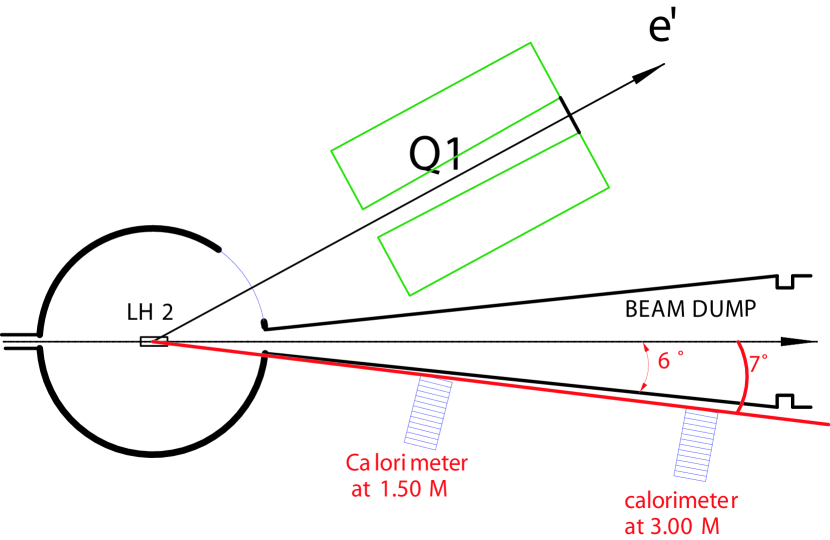
Figure 5: Hall A layout for DVCS with CEBAF at 12 GeV. The scattering chamber is identical to the E00-110 chamber, with a midplane 63 cm radius spherical section with 1 cm Al wall thickness, and a 16 mil Al window facing the HRS L. We propose a conical downstream beam pipe, with half-opening angle of 6 degrees on beam-right, and length 3m. The drawing shows the expanded PbF₂ calorimeter at beam-right, in the closest and farthest configurations: front face 150 cm and 300 cm, respectively, from target center. The calorimeter is shown in its smallest angle setting (inner edge at $7^{\circ}$).

Table 3: Detailed DVCS Kinematics. The first line is from E00-110, and is included for comparison purposes. The angle $\theta_{q}$ is the central angle of the virtual photon direction $q=(k-k^{\prime})$.

$Q^{2}$	$x_{\rm Bj}$	$k$	$k^{\prime}$	$\theta_{e}$	$\theta_{q}$	$q^{\prime}(0^{\circ})$	$W^{2}$
(GeV2)		(GeV)	(GeV)	$({}^{\circ})$	$({}^{\circ})$	(GeV)	(GeV2)
1.90	0.36	5.75	2.94	19.3	18.1	2.73	4.2
3.00	0.36	6.60	2.15	26.5	11.7	4.35	6.2
4.00	0.36	8.80	2.88	22.9	10.3	5.83	8.0
4.55	0.36	11.00	4.26	17.9	10.8	6.65	9.0
3.10	0.50	6.60	3.20	22.5	18.5	3.11	4.1
4.80	0.50	8.80	3.68	22.2	14.5	4.91	5.7
6.30	0.50	11.00	4.29	21.1	12.4	6.50	7.2
7.20	0.50	11.00	3.32	25.6	10.2	7.46	8.1
5.10	0.60	8.80	4.27	21.2	17.8	4.18	4.3
6.00	0.60	8.80	3.47	25.6	14.1	4.97	4.9
7.70	0.60	11.00	4.16	23.6	13.1	6.47	6.0
9.00	0.60	11.00	3.00	30.2	10.2	7.62	6.9

This proposal is based directly on the experience of E00-110. We present a sketch of the DVCS layout in Hall A in Fig. 5. We use the standard 15 cm liquid hydrogen target. We detect the electrons in the HRS-L and photons (and $\pi^{0}\rightarrow\gamma\gamma$) in a PbF₂ calorimeter at beam right. We note in Fig. 5 the modified scattering chamber from E00-110 and a new modified downstream beam pipe. The scattering chamber is 63 cm in radius, with a 1 cm Al spherical wall facing the PbF₂ calorimeter and a thin window (16 mil Al) facing the HRS-L.

The HRS-Left (HRS-L) limits the central values of the scattered electron momentum to

$$k^{\prime} \leq 4.3GeV/c,$$

$$\theta_{e} \geq 12.5^{\circ}.$$ (35)

As detailed in section III.3, to handle both the instantaneous pile-up and integrated radiation dose in the calorimeter, we limit the placement of the calorimeter to

$$\theta_{\rm PbF_{2}}^{\rm min}\geq 7^{\circ}.$$ (36)

At the same time, to ensure adequate azimuthal coverage in $\phi_{\gamma\gamma}$, we limit the placement of the calorimeter

$$\theta_{q}\geq 10^{\circ}.$$ (37)

The following subsections detail our technical solutions, and demonstrate that these technical constraints do not limit the physics scope of this proposal.

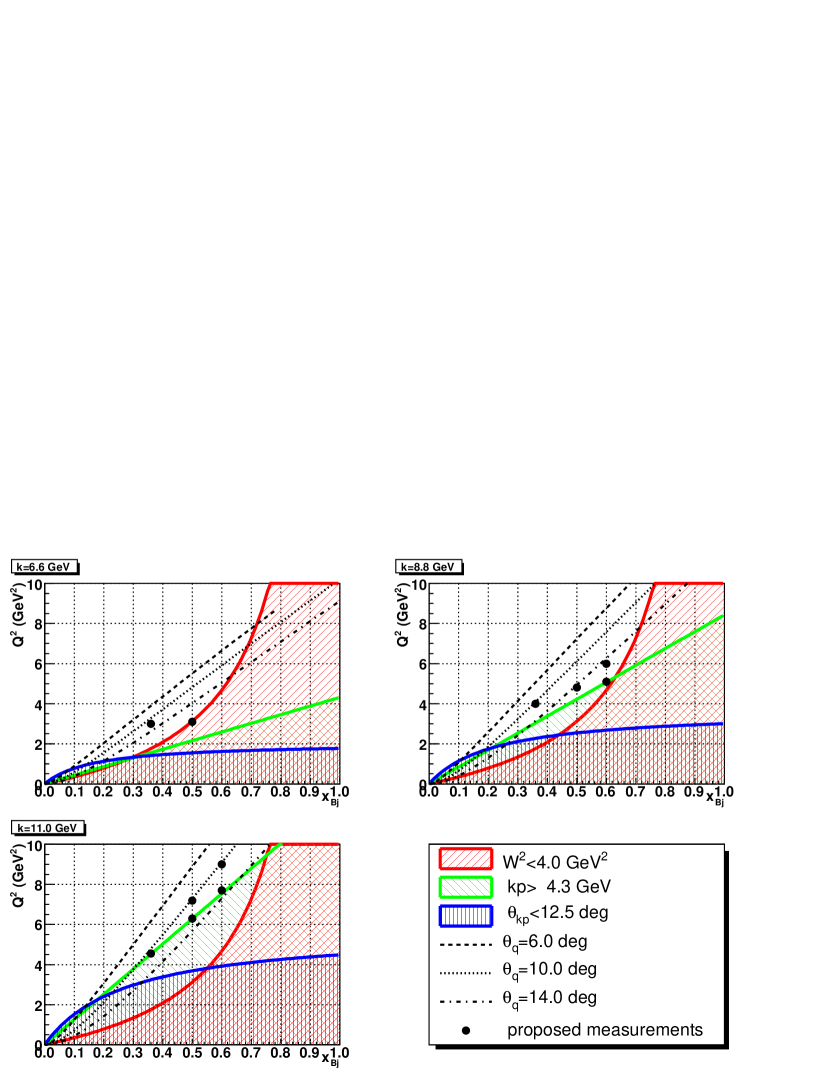
Figure 6: Proposed DVCS central kinematics for H$(e,e^{\prime}\gamma)p$ measurements in Hall A with 6.6, 8.8, and 11 GeV incident beam. The experimental constraints of Eq. 35,37 are indicated. Each experimental point is the center of one of the ’diamond’ regions of Fig. 4.

III.1 High Resolution Spectrometer

Our proposed kinematics, and the physics constraints of Eq. I.3 are illustrated in Fig. 4. The individual beam energies are illustrated in Fig. 6, with the HRS constraints (Eq. 35) superimposed. We note the following points with regard to the HRS and calorimeter (Eq. 37) constraints:

• The HRS constraints have no effect for $Q^{2}>2$ GeV² at $k=6.6$ GeV.

• At $k=8.8$ and 11 GeV, primarily the $k<4.3$ GeV constraint removes roughly the lower half of the $Q^{2}$ range at each $x_{\rm Bj}$. This $Q^{2}$ range for each $x_{\rm Bj}$ is covered by the lower beam energies.

• According to the Base Equipment plan for CEBAF, the three Halls A, B, C, when running simultaneously, must operate at different multiples of 2.2 GeV.

• The small angle calorimeter cut of $\theta_{q}>10^{\circ}$ removes the very highest physically allowed $Q^{2}$ values at each $x_{\rm Bj}$.

• All of the constraints prevent us from kinematics for $x_{\rm Bj}\leq 0.2$.

• Kinematics at $x_{\rm Bj}=0.7$ are allowed at $k=8.8$ and 11 GeV. At this time, it is very difficult to make reliable estimates of the DVCS signal at this extreme $x_{\rm Bj}$, and we do not include these kinematics in our proposal.

The detailed kinematics are summarized in Table 3.

The HRS performance is central to this experiment. Once we make a selection of exclusive H$(e,e^{\prime}\gamma)p$ events, the resolution in $t=(q-q^{\prime})^{2}$ is determined by approximately equal contributions from the HRS momentum resolution and the angular precision of the direction ${\bf\hat{q}^{\prime}}$. The resolution on the direction of ${\bf q}^{\prime}$ has equal contributions from the position resolution in the calorimeter and the vertex resolution, as obtained from the spectrometer. The combination of precise acceptance, kinematic, and vertex resolution in the HRS makes it possible to make precision extractions of the DVCS observables.

III.2 Beam Line

In E00-110 and E03-106, with the front face of the calorimeter 1.10 m from target center, we had a 6” diameter cylindrical beam pipe, welded directly to the scattering chamber. This aperture corresponds to roughly a $6^{\circ}$ half-opening angle from target center. We require placing the calorimeter at distances from 1.5 m to 3.0 m from the target ($\S$III.3). To avoid excess calorimeter background generated by secondaries striking the beam pipe, we propose a thin walled (1/8” Al) conical beam pipe, welded to the same aperture. The cone must be slightly off-axis, to prevent an interference with HRS-Q1 at the minimum spectrometer angle setting of $18^{\circ}$ (Table 3), while at the same time preserving a full $6^{\circ}$ aperture on Beam-right. The cone should be 3.0 m long, to continue downstream of the calorimeter. This will require moving or replacing a gate valve and pumping station.

III.3 PbF₂ Calorimeter

Table 4: Properties of PbF₂.

Density		7.77 g/cm3
Radiation Length		0.93 cm
Molière Radius		2.20 cm
Index of Refraction	($\lambda=180$ nm)	2.05
	($\lambda=400$ nm)	1.82
Critical Energy		9.04 MeV

We will detect the scattered photon in a $13\times 16$ element PbF₂ calorimeter. This is the existing $11\times 12$ E00-110 calorimeter, with 76 additional elements. Each block is $3\times 3$ cm${}^{2}\times 20X_{0}$. The additional blocks will add two more rows on the top and bottom, and two columns on the wide angle side. The properties of PbF₂ are summarized in Table 4. The important design considerations for DVCS are as follows.

• PbF₂ is a radiation hard pure Cerenkov crystal medium Woody et al. (1993);

• With no scintillation lightAnderson et al. (1994), the calorimeter signal is insensitive to low energy nuclear particles, and the pulse rise and fall time is determined only by geometry and the response of the PMT. This allows us to use the 1GHz Analog Ring Sampler (ARS) digitizerF. Feinstein (2003) to minimize pileup.

• The high luminosity of this proposal requires fast response PMTs operated at low gain and capacitively coupled to a pre-amplifier. The low gain reduces the DC anode current. The capacitive coupling removes the average pile-up from low energy $\gamma$-rays.

• The small Molière radius (2.2 cm) allows us to separate closely space showers from $\pi^{0}$ decay, and minimize shower leakage at the boundary.

• The short radiation length minimizes fluctuations in light collection from fluctuations in the longitudinal profile of the shower.

• The low value $9$ MeV of the critical energy (roughly the energy threshold for which bremsstrahlung energy loss exceeds ionization loss for electrons) also improves the resolution e.g. relative to Pb-Glass.

• In E00-110, we obtained a signal of 1 photo-electron per MeV of deposited energy in the E.M. shower, and a energy resolution of 2.4% from elastic H$(e,e^{\prime}_{\text{C}alo}p_{\text{H}RS})$ electron of 4.2 GeV. For our simulations, we project a resolution of $\sigma_{E}/E=2.0\%\oplus(3.2\%)\sqrt{(1\,{\rm GeV})/q^{\prime}}$. We also achieved a spatial resolution of 2 mm at 4.2 GeV. From the combination of energy and spatial resolution, we obtained a $\pi^{0}\rightarrow\gamma\gamma$ mass resolution of 9 MeV.

The size, granularity, and position of the calorimeter must accommodate the following constraints:

1. Nearly $2\pi$ azimuthal photon acceptance for $|\Delta_{\perp}|<0.6$ GeV/c. independent of the central kinematics. The angular size required therefore shrinks as $\Delta_{\perp}^{\rm max}/q^{\prime}(0^{\circ})$.

2. Good separation of the two clusters from the $\pi^{0}\rightarrow\gamma\gamma$ decay, in order to measure the H$(e,e^{\prime}\pi^{0})p$ reaction. For $\pi^{0}\rightarrow\gamma\gamma$ reconstruction, we require a center to center separation of 3 PbF₂ blocks, or 9 cm. In high energy DVCS or deep virtual $\pi^{0}$ kinematics, $q^{\prime}_{\rm DVCS}\approx E_{\pi}$. In this limit, the minimum half opening angle of the $\pi^{0}\rightarrow\gamma\gamma$ decay is $\theta_{\pi\gamma}\geq m_{\pi}/q^{\prime}$. The minimum distance of the calorimeter from the target, based on the cluster separation requirement is given as the $D$ parameter in Table 1. Furthermore, 50% of the $\pi^{0}$ decay events yield both photons within a half angle cone of $\theta_{\pi\gamma}\leq(\sqrt{3/2})(m_{\pi}/q^{\prime})$.

3. Maximum distance from target to minimize pile-up and radiation dose per block at fixed luminosity.

Item 2 requires us to increase $D$ in proportion to $q^{\prime}$. However, from item 1 we see that the acceptance is $\Delta_{\perp}$ remains invariant. The solid angle per PbF₂ block at the distance $D$ determines the maximum feasible luminosity for each setting. Therefore item 3 allows us to increase the luminosity in proportion to $D^{2}\propto q^{\prime\,2}$.

We will calibrate the central blocks of the calorimeter via elastic H$(e,e^{\prime}_{\text{C}alo}p_{\text{H}RS})$ measurements We anticipate three sequences of elastic measurements of one day each at the beginning, middle, and end of each scheduled period of running time. We will then cross calibrate all of the blocks and maintain a continuous monitor of the calibration with the $\pi^{0}$ mass reconstruction from H$(e,e^{\prime}\pi^{0})X$ events. We anticipate sufficient statistics to obtain an independent calibration from each day of running. The elastic calibrations also serve to verify the geometrical surveys of the spectrometer and calorimeter.

III.4 Luminosity Limits and Optical Curing of Calorimeter

In E03-106, we took $D(e,e^{\prime}\gamma)X$ data at a maximum luminosity (per nucleon) of $4\cdot 10^{37}/$cm²/s, with the front face of the PbF₂ calorimeter at 110 cm from the target center. We did not obtain any degradation of resolution in the calorimeter from pileup of signals. During the entire 80 day run of E00-110 and E03-106, we delivered a total of 12 C to the 15 cm liquid Hydrogen and Deuterium targets. We performed absolute calibrations of the calorimeter with elastic H$(e,e_{\rm Calo}^{\prime}p_{\rm HRS})$ events at the beginning and end of data taking. We observed up to 20% decrease in signal amplitude in individual blocks, without observable loss in missing mass resolution after recalibration. Custom pre-amplifiers were used to keep the PMT anode current small. Therefore the loss of amplitude is attributed to degradation of the transmission properties of the blocks, and not to degradation of the photo-cathodes of the PMTs. Independent numericalDegtiarenko (2006) and analytic simulations indicate that below 10 degrees, the radiation dose to the calorimeter is dominated by Møller electrons (and related bremsstrahlung). Beyond 20 degrees, the dominant background arises from decay photons from inclusive $\pi^{0}$ photo-production. The simulations also indicate that from 7.5 to 11.5 degrees, the radiation dose diminishes by a factor 5. On this basis, we conclude that roughly $50\%$ of the radiation dose received by the small angle blocks of the calorimeter occurred when the small angle edge of the calorimeter was at $7^{\circ}$. This is the same minimum angle we will use in the present proposal.

Achenbach et al. studied the radiation damage and optical curing of PbF₂ crystalsAchenbach et al. (1998). They found the radiation damage to be linear for doses up to 8 KGy (from a ⁶⁰Co source). For a dose of 1 KGy, they observed a loss of $25\%$ in transmission for blue light of $\lambda=400$ nm. They also obtained good results for curing the radiation damage by exposure to blue light. The front face of the 1000 element A4 array was exposed for 17 hours to a Hg(Ar) pencil lamp (filtered to pass only $\lambda>365$ nm) at a distance of 50 cm (intensity on the calorimeter surface of $2\,\mu$W/cm²). The transmission of 400 nm and 330 nm light returned to 100% and 97%, respectively, of its initial value.

At this stage, it is not possible to compare the absolute dose in our simulations with the dose recorded in the MAMI-A4 trials. The A4 dose is recorded as a volumetric dose (1Gy = 1Joule/kg) yet the gamma rays from ⁶⁰Co are predominantly absorbed in a layer of thickness 1/10 the transverse size of the crystals. The radiation dose in Hall A during a DVCS experiment is primarily from photons and electrons 50–1000 MeV. Thus we consider the absolute scale of dose comparison to be uncertain by a factor of 10. Instead, we normalize the future radiation damage of the calorimeter to the maximum value for the fractional signal attenuation per integrated luminosity obtained in conditions during E00-110 and E03-106 that were nearly identical our proposed configuration. We utilize the studies from MAMI-A4 to determine that a radiation-dose induced attenuation of up to 25% ($\lambda=400$ nm) can be cured (to within $1\%$) with a 17 hour exposure to blue light. This curing must be followed by several dark hours to allow the phosphorescence of the PMT photo-cathodes to decay.

Pile-up within the 20 ns analysis window of the pulse shape analysis of the PbF₂ signals will limit our instantaneous luminosity. Based on our previous experience we can operate at an instantaneous luminosity times acceptance per PbF₂ block of

$$\mathcal{L}(D) = \left[\frac{(4.0\cdot 10^{37})}{{\rm cm}^{2}\cdot{\rm s}}\right]\,\left[\frac{D}{(110\,{\rm cm})}\right]^{2}.$$ (38)

with $D$ the distance from target to calorimeter. Our projected count rates and beam times are based on this luminosity as a function of the kinematic setting.

We plan to use blue light curing of the blocks every time the signal attenuation reaches $20\%$. For those settings with the minimum edge of the calorimeter $\theta_{\rm Calo}^{\rm min}$ equal to $7^{\circ}$, this corresponds to 5 days of running at the luminosity of Eq. 38. We will use the $\pi^{0}\rightarrow\gamma\gamma$ mass resolution from both single arm H$(e,\pi^{0})Y$ (prescaled) and coincidence H$(e,e^{\prime}\pi^{0})X$ events to monitor the light yields in the PbF₂ array. At larger calorimeter angle settings, the time between curing will be correspondingly longer. We estimate a total of 10–12 curing days during the experiment (in addition to the running time).

III.5 Trigger

The electron detector stack in the HRS will be the standard configuration of VDC I and II, segmented S1 and S2, gas Cerenkov, and Pb-Glass calorimeter. The Cerenkov ($\check{C}er$) and Pb-Glass provide redundant electron identification in the off-line analysis. The main HRS trigger is

$${\rm HRS} = \left[\cup_{i,j}(S1R_{i}\cap S1L_{i})\cap(S2R_{j}\cap S2L_{j})\right]\cap\check{C}er.$$ (39)

This requires a coincidence between the PMTs at the two ends of at least one scintillator paddle in each of $S1$ and $S2$. In addition, we require a coincidence with the Cerenkov counter. Supplementary prescaled triggers with either $S1$, $S2$, or $\check{C}er$ removed from the coincidence will monitor the efficiency of each trigger detector.

In addition to the HRS electron trigger, we will upgrade our present coincidence validation/fast-clear logic. The calorimeter signals are continuously recorded by the 128 sample $\otimes$ 1GHz ARS F. Feinstein (2003); Roblin et al. (2000) array. This array is digitized, at a slower rate, following a trigger validation. For each HRS trigger, we stop the ARS sampling, and trigger a Sample and Hold (SH) circuit, that is coupled to the calorimeter signals via a high impedance input (in the future, we may replace this with a pipeline ADC). The SH signals are digitized and then in a field programmable gate array (FPGA), we will form the following trigger validation signals.

1. A validation of the HRS-electron trigger, based on detecting at least one $2\times 2$ cluster above a programmable threshold $E_{\gamma}^{\rm Th}$.

2. A $\pi^{0}$ trigger based on detecting at least two separated $2\times 2$ clusters, with each cluster above a programmable threshold $E_{1}$ and the sum of the two clusters above a programmable threshold $E_{\pi}$. This trigger will select candidate H$(e,e^{\prime}\pi^{0})X$ events.

If a valid signal is found, the ARS array is digitized and recorded (together with the HRS signals). If the HRS trigger is not validated by the calorimeter signals, a fast clear is issued to the ARS array, no digitization occurs, and acquisition resumes. During E00-110, the SH/Fast-clear cycle took 500 ns. With upgrades to the FPGA, we can shorten this deadtime by a factor of two. In addition, upgrades to the VME standard will allow us to increase the total bandwidth of data acquisition for this proposal.

IV Projected Results

Table 5: Experimental Conditions for DVCS. For each $(Q^{2},k,x_{\rm Bj})$ setting, we present: Maximum photon energy $q^{\prime}(0^{\circ})$; Calorimeter distance $D$; Virtual photon direction $\theta_{q}$; Angle $\theta_{calo}^{min}$ of the edge of the calorimeter, relative to the beam line; Kinematic minimum $|t_{\rm min}|$ and upper bound $|t_{\rm max}|$ for approximately full acceptance in $\phi_{\gamma\gamma}$; Resolution $\sigma(M_{X}^{2})$ in H$(e,e^{\prime}\gamma)X$ missing mass squared; Luminosity $\mathcal{L}$; H$(e,e)X$ inclusive trigger rate, H$(e,e^{\prime}\gamma)p$ exclusive DVCS count rate. The beam time is calculated to obtain an estimated 250K events at each setting, or at least 40,000 events per bin in $t_{\rm min}-t$. The distance $D$ of the front face of the calorimeter from the target center is optimized for the separation of the clusters from $\pi^{0}\rightarrow\gamma\gamma$ decay (section III.3). The intrinsic missing mass resolution in E00-110 is $\sigma(M_{X}^{2})=0.20$ GeV². The luminosity is determined by the maximum rate allowed by pileup in the calorimeter. This luminosity is proportional to $D^{2}$ ($\S$III.4).

$Q^{2}$	$k$	$x_{\rm Bj}$	$q^{\prime}(0^{\circ})$	$D$	$\theta_{q}$	$\theta_{calo}^{min}$	$t_{min}$	$t_{max}$	$\sigma(M_{X}^{2})$	${\mathcal{L}}/10^{38}$	HRS	DVCS	Time
(GeV2)	(GeV)		(GeV)	(m)	(deg)	(deg)	(GeV2)	(GeV2)	(GeV2)	(cm-2/s)	(Hz)	(Hz)	(days)
3.0	6.6	0.36	4.35	1.5	11.7	7.1	-0.16	-0.42	0.23	0.75	479	1.16	3
4.0	8.8	0.36	5.83	2.0	10.3	7.0	-0.17	-0.42	0.26	1.3	842	1.74	2
4.55	11.0	0.36	6.65	2.5	10.8	7.0	-0.17	-0.42	0.27	2	2460	4.63	1
3.1	6.6	0.5	3.11	1.5	18.5	11.0	-0.37	-0.64	0.17	0.75	873	0.77	5
4.8	8.8	0.5	4.91	2.0	14.5	8.9	-0.39	-0.70	0.20	1.3	716	0.82	4
6.3	11.0	0.5	6.50	2.5	12.4	7.9	-0.40	-0.72	0.20	2.	778	0.99	4
7.2	11.0	0.5	7.46	2.5	10.2	7.0	-0.40	-0.75	0.25	2.	331	0.53	7
5.1	8.8	0.6	4.18	1.5	17.8	10.4	-0.65	-1.06	0.16	0.75	338	0.27	13
6.0	8.8	0.6	4.97	2.0	14.8	9.2	-0.67	-1.05	0.18	1.3	227	0.22	16
7.7	11.0	0.6	6.47	2.5	13.1	8.6	-0.69	-1.10	0.20	2.	274	0.28	13
9.0	11.0	0.6	7.62	3.0	10.2	7.3	-0.71	-1.14	0.22	3.	117	0.17	20

The detailed $(e,e^{\prime})$ kinematics, calorimeter configuration, H$(e,e^{\prime}\gamma)X$ missing mass resolution in $M_{X}^{2}$, count-rates, and beam time are summarized in Table 5. The beam time is chosen to give a total statistics of 250K events per $(x_{\rm Bj},Q^{2})$ setting.

IV.1 Systematic (Instrumental) Errors

Table 6 shows the main systematic errors on the cross-sections extraction during estimation of those errors for the proposed experiment. The main improvements of the errors are due to :

• The beam polarization measurements: the upgrade of the Compton polarimeter along the Hall A beam line will reduce the relative precision $\Delta P/P$ from 2% to 1%. The average beam polarization for E00-110 was 75% and is expected to be 85% for the proposed experiment.

• Drift chamber multi-tracks : the number of events for which multiple tracks are reconstructed in the focal plane of the HRS is proportional to the single rates. Multiple tracks events are discarded during the analysis and the live time of the experiment corrected accordingly. Because the proposed experiment is measured deeper in the DIS region, we expect that the correction will be smaller as well as its uncertainty.

• $\pi^{0}$ subtraction : the limitation on the precision of the correction for E00-110 was both statistical and limited by the kinematical range of the recorded $\pi^{0}$ events. For the proposed experiment, we plan to improve the trigger such that more $\pi^{0}$ events are recorded. A special trigger with lower threshold but the requirement of two clusters being above it, will be implemented.

• e(p,e’$\gamma$)$\pi$N contamination : the missing mass squared resolution is the key ingredient for this contamination. The proposed estimation takes into account the variation of this resolution for the new kinematics.

The systematic errors in Table 6 are summarized separately for the cross section sum $d\overrightarrow{\sigma}+d\overleftarrow{\sigma}$, and for the cross section difference $d\overrightarrow{\sigma}-d\overleftarrow{\sigma}$.

Type		Relative errors (%)
		E00-110	proposed
Luminosity	target length and beam charge	1	1
HRS-Calorimeter	Drift chamber multi-tracks	1.5	1
	Acceptance	2	2
	Trigger dead-time	0.1	0.1
DVCS selection	$\pi^{0}$ subtraction	3	1
	e(p,e’$\gamma$)$\pi$N contamination	2	3
	radiative corrections	2	1
Total cross section sum		4.9	4.1
Beam	Polarization $\Delta P/P$	2	1
Total cross section difference		5.3	4.2

Table 6: Relative systematic error budget for E00-110 and for the proposed experiment.

IV.2 Statistics

Fig. 7–9 show acceptance, counting statistics, and cross section distributions for specific $(x_{\rm Bj},Q^{2})$ kinematics. In each figure, we present the cross section weighted acceptance distribution of a basic set of kinematic variables in the upper left panel. The central plot of this panel is the H$(e,e^{\prime}\gamma)X$ missing mass squared $M_{X}^{2}$ distribution for simulated exclusive events. The blue curve is a simulation for E00-110. The missing mass resolution $\sigma(M_{X}^{2})$ for each setting is tabulated in Table 5. For E00-110, the resolution is $\sigma(M_{X}^{2})=0.20$ GeV². In the lower right kinematic plot, The green rectangle is the fiducial surface of $11\times 14$ blocks of the calorimeter (we require the centroid of EM shower to be a a minimum of of one block from the calorimeter edge). The points in red on this plot show the distribution of directions of the ${\bf q}$-vector. The upper right panel of the figures shows the counting statistics (helicity sum and helicity difference) as functions of $\phi_{\gamma\gamma}$ for five bins in $t$. As $-t$ increases from left to right, the simulation shows the gradual loss of acceptance for $\phi_{\gamma\gamma}$ near $0^{\circ}$, due to the off-centered calorimeter. The bottom right panel shows the projected helicity sum and helicity difference cross sections, with statistical errors, in the same bins in $t$ and $\phi_{\gamma\gamma}$. The statistics are for the projected beam time of this proposal. These estimates were made with our simulation code TCHIB. The cross section model for these estimates is described in §IV.3.

With 250K events in each $(x_{\rm Bj},Q^{2})$ setting, we obtain a high precision determination of all the observables detailed in the Section II.4.

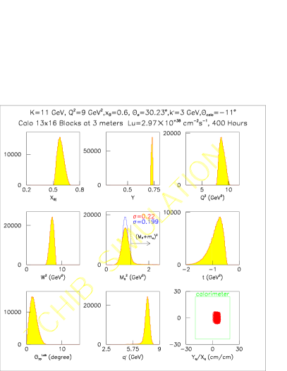
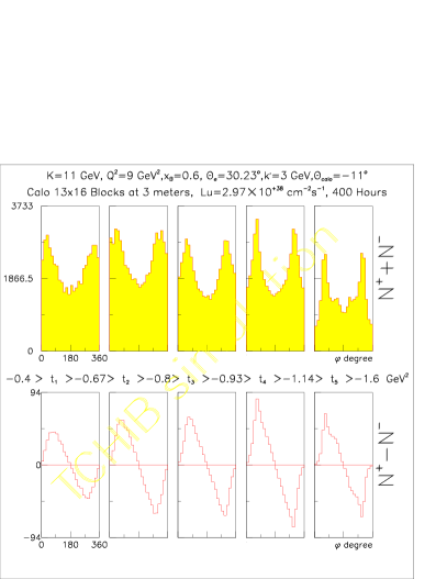
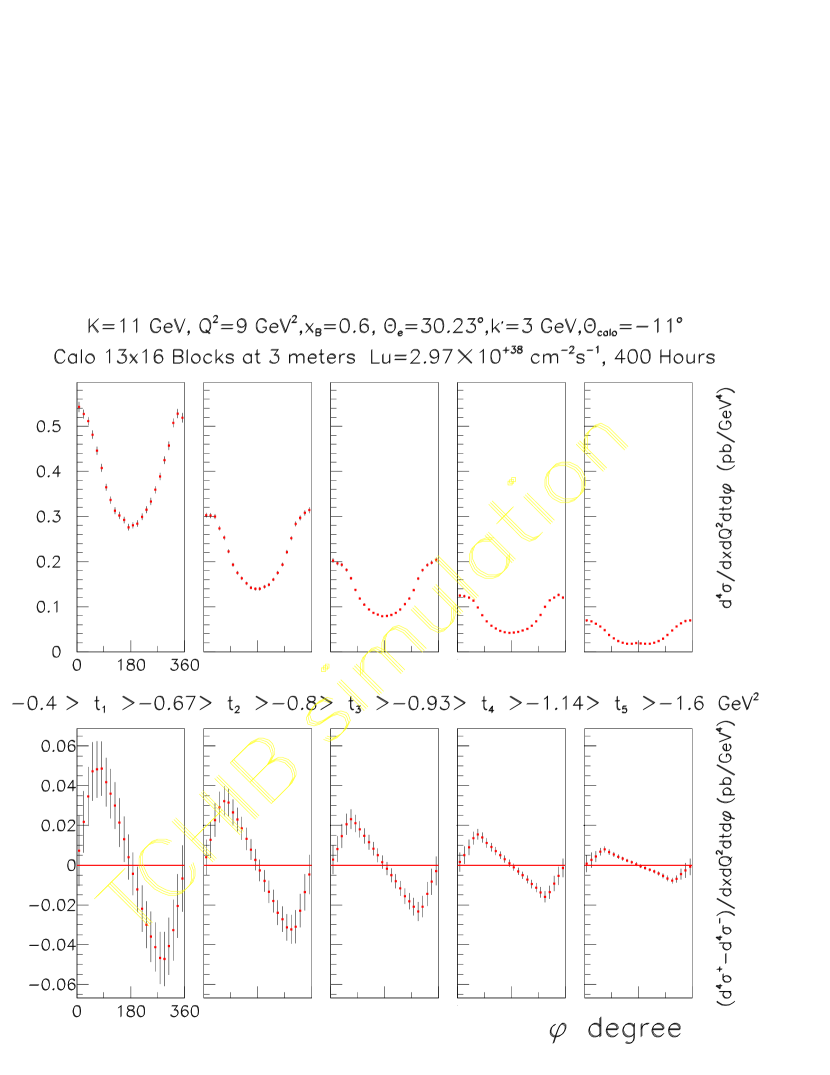
Figure 7: DVCS Distributions for setting $k=11$ GeV, $Q^{2}=9$ GeV², $x_{\rm Bj}=0.6$.
Top Left: Cross section weighted acceptance distributions.
Top Right: Helicity sum and helicity difference projected counts as a function of $\phi_{\gamma\gamma}$ in five bins in $t$.
Bottom Right: Helicity sum and helicity difference projected cross sections, with statistical uncertainties, as functions of $\phi_{\gamma\gamma}$ in the same bins in $t$.

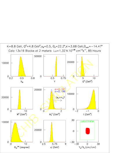
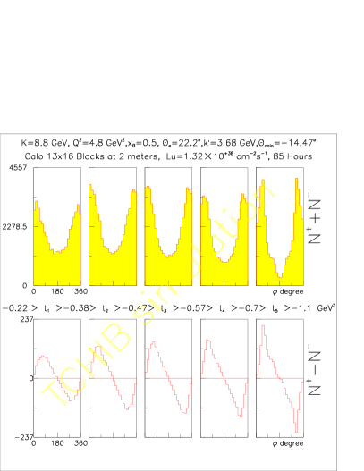
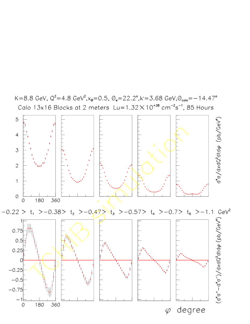
Figure 8: DVCS Distributions for setting $k=8.8$ GeV, $Q^{2}=4.8$ GeV², $x_{\rm Bj}=0.5$.
Top Left: Cross section weighted acceptance distributions.
Top Right: Helicity sum and helicity difference projected counts as a function of $\phi_{\gamma\gamma}$ in five bins in $t$.
Bottom Right: Helicity sum and helicity difference projected cross sections, with statistical uncertainties, as functions of $\phi_{\gamma\gamma}$ in the same bins in $t$.

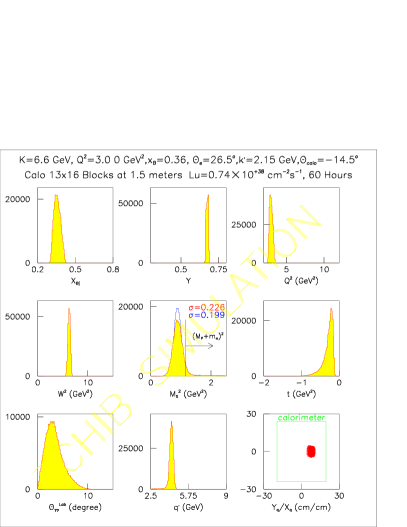
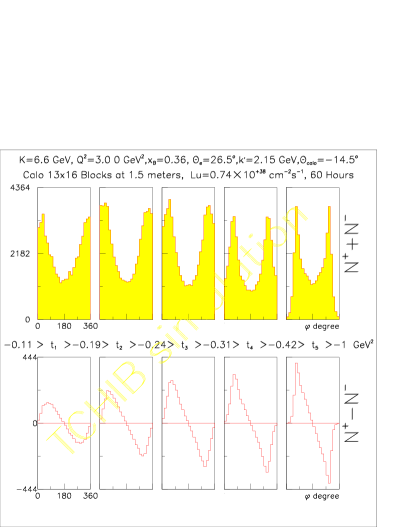
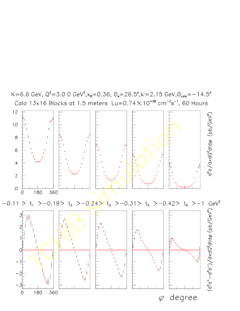
Figure 9: DVCS Distributions for setting $k=6.6$ GeV, $Q^{2}=3.0$ GeV², $x_{\rm Bj}=0.36$.
Top Left: Cross section weighted acceptance distributions.
Top Right: Helicity sum and helicity difference projected counts as a function of $\phi_{\gamma\gamma}$ in five bins in $t$.
Bottom Right: Helicity sum and helicity difference projected cross sections, with statistical uncertainties, as functions of $\phi_{\gamma\gamma}$ in the same bins in $t$.

IV.3 Illustration of Prospective Physics

In each setting $(x_{\rm Bj},Q^{2})$ setting, we will extract in the $t$-bins defined in Fig. 7–9, the experimental Twist-2 and Twist-3 BH$\cdot$DVCS interference observables defined in Section. II.4. In addition, we will obtain upper bounds on the gluon transversity terms $\cos(3\phi_{\gamma\gamma})$ and $\sin(3\phi_{\gamma\gamma})$.

We illustrate the possible $x_{\rm Bj}$-dependence of the Twist-2 coefficients in Fig. 10. The principal-value integrals in the $\Re\text{e}\mathcal{C}^{\mathcal{I}}$ and $\Re\text{e}\Delta\mathcal{C}^{\mathcal{I}}$ must change sign somewhere in the range $0\leq\xi<1$. In Fig. 11, we present the impact on $\Im\text{m}[\mathcal{C}^{\mathcal{I}}]$ of the DGLAP evolution of $H(x,\xi,t;Q^{2})$ in the VGG model Vanderhaeghen et al. (1999); Goeke et al. (2001); Guidal et al. (2005). The VGG model uses the double distributions for $H$:

$$H_{f}(x,\xi,t) = \int d\beta d\alpha\delta(x-\beta-\alpha\xi)F_{f}(\beta,\alpha,t)$$ (40)

$$F_{f}(\beta,\alpha,t) = \left.h(\beta,\alpha)q_{f}(\beta)\right/\beta^{\alpha^{\prime}t}$$ (41)

$$h(\beta,\alpha) = C(b)\left[(1-|\beta|)^{2}-\alpha^{2}\right]^{b}\left/\left(1-|\beta|\right)^{2b+1}\right.$$ (42)

The limits of integration in Eq. 40, and the normalization constant $C(b)$ are defined in Goeke et al. (2001). In these illustrative plots, we have taken the profile parameter $b=1$ and the Regge parameter $\alpha^{\prime}=0.8$ GeV^-2. A similar form is used for $\tilde{H}$, with $q_{f}(\beta)$ replaced with $\Delta q_{f}(\beta)$. We also set $E=0$ in these figures. For our count rate estimates in the previous section, we have used the factorized ansatz which is obtained in the $b\rightarrow\infty$ limit. In Fig. 11, the DGLAP evolution is applied only to the parton distributions $q_{f}(\beta)$. We note that the experimental contribution of the Twist-3 term $\langle\eta_{1}\rangle\Im\text{m}[\mathcal{C}_{1}^{\rm DVCS}]$ (Eq. 30) will decrease in proportion to $1/\sqrt{Q^{2}}$. At the same time, higher twist contributions in $\Im\text{m}[\mathcal{C}^{\mathcal{I}}]$ will decrease in proportion to $1/Q^{2}$ (or higher powers). Thus it should be possible to extract the Twist-2 and Twist-3 contributions from the $Q^{2}$-dependence, with only a small model dependence from the distinct QCD evolution of the three contributing GPDs.

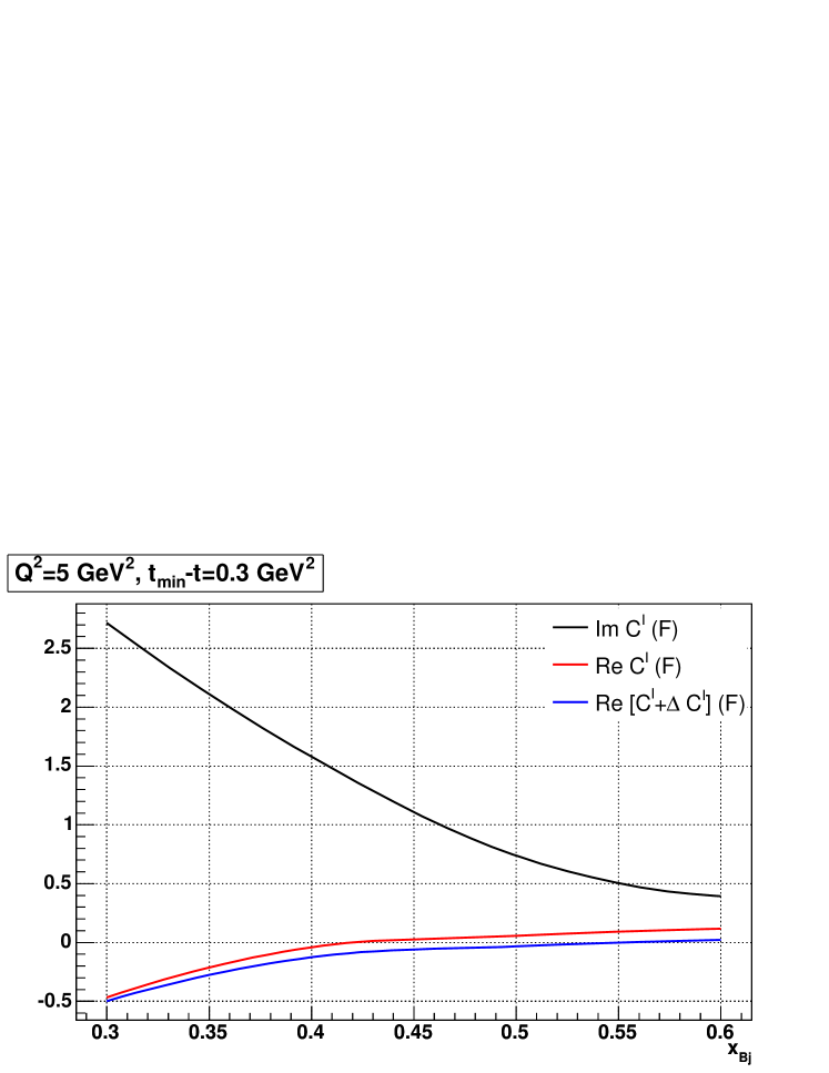
Figure 10: The three Twist-2 observables, as functions of $x_{\rm Bj}$ at $t_{\text{m}in}-t=0.3$ GeV². The model is from VGG Vanderhaeghen et al. (1999); Goeke et al. (2001); Guidal et al. (2005).

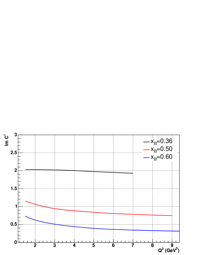
Figure 11: QCD evolution of $\mathcal{C}^{\mathcal{I}}$, as obtained from DGLAP evolution of $H(x,\xi,t;Q^{2})$ in the VGG model Vanderhaeghen et al. (1999); Goeke et al. (2001); Guidal et al. (2005).

Fig. 12 illustrates the $t$-dependence of $\Im\text{m}\mathcal{C}^{\mathcal{I}}(\mathcal{F})$, plotted here as a function of $t_{\text{m}in}-t$ for our three values of $x_{\rm Bj}$. The $t$-dependence of this observable is the bilinear combination of the Compton form factors with the proton form factors in the BH amplitude.

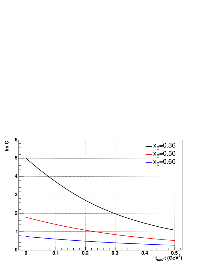
Figure 12: Dependence of $\Im\text{m}\mathcal{C}^{\mathcal{I}}(\mathcal{F})$ as a function of $t_{\text{m}in}-t$ for the three values of $x_{\rm Bj}$ of this proposal at constant $Q^{2}$. The curves are obtained from the contributions of $H(x,\xi,t)$ and $\tilde{H}(x,\xi,t)$ in the VGG model Vanderhaeghen et al. (1999); Goeke et al. (2001); Guidal et al. (2005).

V Summary

With a high precision spectrometer, and a compact, hermetic high-performance calorimeter in Hall A, we can obtain high statistics absolute measurements of $\vec{e}p\rightarrow ep\gamma$ cross sections in a wide DVCS kinematic domain with CEBAF at 12 GeV. We expect to obtain precision measurements of three Twist-2 DVCS observables and two Twist-3 DVCS observables. The $Q^{2}$ dependence will provide stringent tests of the factorization theorem, and quantify the contribution of higher twist terms (which can be modelled as the hadronic content of the photon). The $t$-dependence as a function of $x_{\rm Bj}$ (or $\xi$) of the observables will provide our first study of transverse profile of the proton as a function of quark light-cone momentum fraction. We note that in this kinematic region, models such as the VGG model presented in §IV.3 must be considered uncertain by at least a factor of two. Our separations of the $\Re\text{e}$ and $\Im\text{m}$ parts of the DVCS observables will provide a calibration for present and future measurements of relative asymmetries. Through the principle value integrals, the $\Re\text{e}$ part provides access to regions of $(x,\xi)$-space that are not directly accessible via the $\Im\text{m}$ part of the GPDs. The $\Im\text{m}$ part observables restrict the GPDs to the sum of the points $x=\pm\xi$.

We will obtain precision measurements of the $\sigma_{L}+\sigma_{T}/\epsilon_{L}$, $\sigma_{LT}$, $\sigma_{TT}$ and $\sigma_{LT^{\prime}}$ cross sections of neutral pion electro-production H$(e,e^{\prime}\pi^{0})p$. The factor $\epsilon_{L}$ is the degree of longitudinal polarization of the virtual photon.. The transverse cross section $\sigma_{T}$ is expected to fall faster with $Q^{2}$ (by one power of $1/Q^{2}$) than the leading twist term in the longitudinal cross section $d\sigma_{L}$. Therefore, from the $Q^{2}$ dependence of the H$(e,e^{\prime}\pi^{0})p$ cross section, we can extract the leading twist (handbag) contribution to this process.

We require 88 days of production running, with an anticipated additional 12 days interlaced for optical curing of the calorimeter. This will provide a major survey of proton DVCS in almost the entire kinematic range accessible with CEBAF at 12 GeV.

REFERENCES

Appendix A Contributions to Hall A Equipment for 11 GeV

Our committments to the Hall A Base Equipment are detailed in Table 7. The collaboration will also seek additional funds for the upgrade to the calorimeter and beam line.

Table 7: Contributions of DVCS Collaboration to Hall A Base Equipment

Institution	Funding Source	Project Description	Equipment
LPC-Clermont-Ferrand	IN2P3-CNRS	Compton Polarimeter:	$125K
		HRS Trigger Electronics	$39K
Technical Manpower for Base Equipment			(months)
LPC-Clermont-Ferrand	IN2P3-CNRS	Compton Polarimeter:
		E  ngineer .	24
		T  echnician	24
		P  hysicist .	12
		HRS Trigger Electronics
		E  ngineer .	6
		T  echnician	6
Old Dominion U.	DOE	HRS DAQ Faculty	4
	(ongoing grant)	PostDoc	12

Appendix B Preparation of Extensions

We are actively preparing a number of extensions of this proposal, which will lead to a comprehensive program of measurements exploiting the unique capabilities of Hall A.

B.1 Deuterium

We currently have preliminary quasi-free and coherent DVCS data from Hall A E03-106 in the channels D$(e,e^{\prime}\gamma)pn\oplus{\rm D}(e,e^{\prime}\gamma)D$. These two channels are (partially) separated experimentally by the differential recoil of the coherent deuteron. In a plot of $M_{X}^{2}$, calculated for H$(e,e^{\prime}\gamma)p$ kinematics, the coherent Deuteron peak appears at $M_{X}^{2}=M_{p}^{2}+t/2$ (Fig. 13). The smearing of the quasi-elastic D$(e,e^{\prime}\gamma)pn$ events by the internal momentum distribution of the $np$ wavefunction of the deuteron is less than our experimental resolution. Thus our isolation of the D$(e,e^{\prime}\gamma)pn$ channel from the inelastic D$(e,e^{\prime}\gamma)NN\pi$ channel is only slightly degraded compared to the identification of the H$(e,e^{\prime}\gamma)p$ exclusive channel.

In a Quasi-Free (QF) model, the neutron DVCS cross section can be obtained from the following subtraction:

$$d^{5}\sigma(\vec{e}n\rightarrow e^{\prime}\gamma n)= d^{5}\sigma(\vec{e}D\rightarrow e^{\prime}\gamma np)-d^{5}\sigma(\vec{e}p\rightarrow e^{\prime}\gamma p)$$ (43)

All observables on the neutron have the same form as for the proton. Using isospin symmetry, the neutron observables interchange the role of up and down quarks. Whereas the proton cross sections are four times more sensitive to up than down quarks, the reverse is true for the neutron. As a consequence, based on the forward parton limits of the GPDs and the Form Factor constraints of the first moments of the GPDs, we expect the neutron observable $\mathcal{C}^{\mathcal{I}}$ to be dominated by the GPD $E$.

In Fig. 13, we show the helicity correlated statistics in three zones in missing mass of the ’neutron’ spectrum of Eq. 43. We note that the signal obtained in the ’$NN$-coherent’ region $M_{X}^{2}<0.6$ GeV² is of opposite sign from the signal in the Quasi-Free region near $M_{X}^{2}=M^{2}$.

We expect to prepare a separate proposal for $D(e,e^{\prime}\gamma)$ measurements for the next 12 GeV PAC. We expect the Deuterium proposal to include a subset of the present kinematics. We would propose to run the two experiments concurrently, with alternating sequences of Hydrogen and Deuterium data taking, to minimize systematic errors.

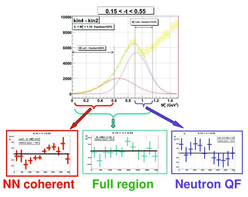
Figure 13: Top: Missing mass distribution of E03-106 D$(e,e^{\prime}\gamma)X$ events, after subtracting a normalized ensemble of H$(e,e^{\prime}\gamma)X$ events. The kinematics are $Q^{2}=1.9$ GeV², $x_{\rm Bj}=0.36$, and $\langle t\rangle=-0.3$ GeV². The missing mass is calculated for $N(e,e^{\prime}\gamma)N$ kinematics. Thus the quasi-free $n(e,e^{\prime}\gamma)n$ peak appears at $M_{X}^{2}=M^{2}$ and and the coherent D$(e,e^{\prime}\gamma)$D peak is broadened by the $t$-acceptance of the events, and appears at $M_{X}^{2}=M^{2}+t/2$. In the region $M_{X}^{2}>M^{2}+t/2$, there can also be a contribution from D$(e,e^{\prime}\gamma)np$ on high momentum correlations in the initial state of the Deuteron (’$NN$-Coherent’). The curves are a two-gaussian fit, with the relative positions constrained to $t/2$. The bottom three plots show the helicity weighted statistics $N(+)-N(-)$ in the three missing mass regions: $0.0<M_{X}^{2}<0.6$ GeV² (left); $0.0<M_{X}^{2}<1.15$ GeV² (center); and $0.9<M_{X}^{2}<1.15$ GeV² (right). The ’$NN$-coherent’ and ’Quasi-Free Neutron’ regions have opposite asymmetry.

B.2 Recoil Polarimetry

A full DVCS program requires proton polarization measurements. and detection of nuclear recoils in coherent $A(e,e\gamma A)$ DVCS reactions. The single- and double-spin observables of proton recoil polarization in $\vec{e}p\rightarrow e^{\prime}\vec{p}\gamma$ and functionally equivalent to the observables for polarized targets: $\vec{e}\vec{p}\rightarrow e^{\prime}p\gamma$ (D. Müller, private communication 2006). We are working on a conceptual design for a large acceptance recoil polarimeter. With an analyzer of 7 cm C, we can achieve a Figure of Merit $\geq 0.005$ (scattering probability times analyzing power squared) for $p_{p}>550$ MeV/c. This could measure both longitudinal and transverse recoil proton polarization in DVCS. This would operate in an axial magnetic field at high luminosity in Hall A, in conjunction with the equipment of this proposal. We intend to have a proposal ready for PAC 32. (Summer 2007).

REFERENCES

- Ji (1997) X.-D. Ji, Phys. Rev. Lett. 78, 610 (1997), eprint hep-ph/9603249.
- Radyushkin (1997) A. V. Radyushkin, Phys. Rev. D56, 5524 (1997), eprint hep-ph/9704207.
- Mueller et al. (1994) D. Mueller, D. Robaschik, B. Geyer, F. M. Dittes, and J. Horejsi, Fortschr. Phys. 42, 101 (1994), eprint hep-ph/9812448.
- Ji and Osborne (1998) X.-D. Ji and J. Osborne, Phys. Rev. D58, 094018 (1998), eprint hep-ph/9801260.
- Collins and Freund (1999) J. C. Collins and A. Freund, Phys. Rev. D59, 074009 (1999), eprint hep-ph/9801262.
- Belitsky et al. (2002) A. V. Belitsky, D. Mueller, and A. Kirchner, Nucl. Phys. B629, 323 (2002), eprint hep-ph/0112108.
- Diehl et al. (1997) M. Diehl, T. Gousset, B. Pire, and J. P. Ralston, Phys. Lett. B411, 193 (1997), eprint hep-ph/9706344.
- Burkardt (2000) M. Burkardt, Phys. Rev. D62, 071503 (2000), eprint hep-ph/0005108.
- Ralston and Pire (2002) J. P. Ralston and B. Pire, Phys. Rev. D66, 111501 (2002), eprint hep-ph/0110075.
- Diehl (2002) M. Diehl, Eur. Phys. J. C25, 223 (2002), eprint hep-ph/0205208.
- Belitsky et al. (2004) A. V. Belitsky, X.-d. Ji, and F. Yuan, Phys. Rev. D69, 074014 (2004), eprint hep-ph/0307383.
- Aktas et al. (2005) A. Aktas et al. (H1), Eur. Phys. J. C44, 1 (2005), eprint hep-ex/0505061.
- Adloff et al. (2001) C. Adloff et al. (H1), Phys. Lett. B 517, 47 (2001), eprint hep-ex/0107005.
- Chekanov et al. (2003) S. Chekanov et al. (ZEUS), Phys. Lett. B573, 46 (2003), eprint hep-ex/0305028.
- Stepanyan et al. (2001) S. Stepanyan et al. (CLAS), Phys. Rev. Lett. 87, 182002 (2001), eprint hep-ex/0107043.
- Airapetian et al. (2001) A. Airapetian et al. (HERMES), Phys. Rev. Lett. 87, 182001 (2001), eprint hep-ex/0106068.
- Ellinghaus (2002) F. Ellinghaus (HERMES), Nucl. Phys. A711, 171 (2002), eprint hep-ex/0207029.
- Airapetian et al. (2006) A. Airapetian et al. (HERMES) (2006), eprint hep-ex/0605108.
- Chen et al. (2006) S. Chen, H. Avakian, V. Burkert, and P. Eugenio (CLAS) (2006), eprint hep-ex/0605012.
- Roblin et al. (2000) Y. Roblin et al. (the Hall A DVCS Collaboration) (2000), JLab Experiment E00-110, Deeply Virtual Compton Scattering at 6 GeV, URL http://hallaweb.jlab.org/experiment/DVCS/dvcs.pdf.
- Voutier et al. (2003) E. Voutier et al. (the Hall A DVCS Collaboration) (2003), JLab Experiment E03-106, Deeply virtual Compton Scattering on the Neutron, URL http://hallaweb.jlab.org/experiment/DVCS/ndvcs.pdf.
- Muñoz Camacho et al. (2006) C. Muñoz Camacho et al. (Hall A DVCS) (2006), eprint nucl-ex/0607029.
- Schaefer et al. (2001) S. Schaefer, A. Schafer, and M. Stratmann, Phys. Lett. B514, 284 (2001), eprint hep-ph/0105174.
- Osipenko et al. (2005) M. Osipenko et al., Phys. Lett. B609, 259 (2005), eprint hep-ph/0404195.
- Eidelman et al. (2004) S. Eidelman et al. (Particle Data Group), Phys. Lett. B592, 1 (2004), URL pdg.lbl.gov.
- Bauer et al. (1978) T. H. Bauer, R. D. Spital, D. R. Yennie, and F. M. Pipkin, Rev. Mod. Phys. 50, 261 (1978).
- Burkardt (2004) M. Burkardt, Phys. Lett. B595, 245 (2004), eprint hep-ph/0401159.
- Burkardt and Miller (2003) M. Burkardt and G. A. Miller (2003), eprint hep-ph/0312190.
- Bacchetta et al. (2004) A. Bacchetta, U. D’Alesio, M. Diehl, and C. A. Miller, Phys. Rev. D70, 117504 (2004), eprint hep-ph/0410050.
- Woody et al. (1993) C. Woody et al., IEEE Trans. Nucl. Sci. 40, 546 (1993).
- Anderson et al. (1994) D. F. Anderson, J. A. Kierstead, S. Stoll, C. L. Woody, and P. Lecoq, Nucl. Instrum. Meth. A342, 473 (1994).
- F. Feinstein (2003) F. Feinstein, Nucl. Instrum. Meth. A504, 258 (2003).
- Degtiarenko (2006) P. Degtiarenko (2006), private communication, URL www.jlab.org/~pavel/cehw.
- Achenbach et al. (1998) P. Achenbach et al., Nucl. Instrum. Meth. A416, 357 (1998).
- Vanderhaeghen et al. (1999) M. Vanderhaeghen, P. A. M. Guichon, and M. Guidal, Phys. Rev. D60, 094017 (1999), eprint hep-ph/9905372.
- Goeke et al. (2001) K. Goeke, M. V. Polyakov, and M. Vanderhaeghen, Prog. Part. Nucl. Phys. 47, 401 (2001), eprint hep-ph/0106012.
- Guidal et al. (2005) M. Guidal, M. V. Polyakov, A. V. Radyushkin, and M. Vanderhaeghen, Phys. Rev. D72, 054013 (2005), eprint hep-ph/0410251.