Study of $\omega$–meson production in pp collisions at ANKE

Abstract

The production of $\omega$-mesons in the $pp\to{}pp\omega$ reaction has been investigated with the COSY–ANKE spectrometer for excess energies of 60 and 92 MeV by detecting the two final protons and reconstructing their missing mass. The large multipion background was subtracted using an event-by-event transformation of the proton momenta between the two energies. Differential distributions and total cross sections were obtained after careful studies of possible systematic uncertainties in the overall ANKE acceptance. The results are compared with the predictions of theoretical models. Combined with data on the $\phi$-meson, a more refined estimate is made of the Okubo-Zweig-Iizuka rule violation in the $\phi/\omega$ production ratio.

1 Introduction

The nucleon–nucleon system is strongly coupled to channels that contain one or multiple mesons. The production of these in $NN$-collisions, preferably near their respective thresholds, will test and constrain theoretical models since, in these cases, only few partial waves contribute. The production of pions and heavier pseudoscalar mesons including kaons has been systematically studied in proton-proton interactions in the near–threshold region Hanhart . Now vector mesons, such as the $\rho$ and the $\omega$, are significant contributors to the $NN$ force at short distances but for these particles much less information is available on their production mechanism due to the lack of experimental data. The relative production of the isoscalar $\omega$ and $\phi$ mesons has recently received renewed interest in connection with the so–called Okubo–Zweig–Iizuka (OZI) rule OZI . This ratio may give information on the admixture of strange quarks in the nucleon only if the production mechanism is known to be the same for both mesons Nakayama ; Kampfer ; Fuchs . This can be best controlled through near–threshold measurements but, as yet, the experimental data set is rather limited.

In the $\omega$ case, the $pp\to{}pp\omega$ total cross section was measured for excess energies $Q\leq 30\,$MeV at SATURNE by detecting the two protons in the SPESIII magnetic spectrometer and identifying the meson by the missing–mass method SPES . In a more exclusive experiment, the DISTO collaboration also measured $\omega$ production but at much higher energy ($Q\approx 320\,$MeV) DISTO . The only data between were taken at COSY–TOF, a non–magnetic time–of–flight spectrometer, where the reaction was studied at $Q=92$ and 173 MeV TOF . This latter energy is in fact the lowest for which differential distributions are available. Extra data are therefore required to fill the gap and confirm the energy dependence. For this purpose we here present $\omega$ results obtained using the COSY–ANKE facility at 60 and 92 MeV. It is relevant within the OZI context to note that the DISTO group measured $\phi$ production at 82 MeV, and we have recently published similar data at 18.5, 34.5, and 75.9 MeV Hartmann .

The experimental facility at our disposal is described in section 2, where particle identification and efficiency determination, as well as the extraction of the luminosity, are also discussed. Since the $\omega$-meson production is identified from the missing mass of two final protons, one of the major problems is a large background under the $\omega$ peak arising from the production of two or more pions. We use the same kinematic transformation as proposed in the SPESIII analysis to estimate this multipion background by employing data obtained at the other energy. This is the crucial element of the $pp\rightarrow{}pp\omega$ event selection, which is treated in detail in section 3. The acceptance of the two protons from the $pp\to{}pp\omega$ reaction in ANKE was far from complete and so a thorough investigation of various one–dimensional differential distributions was undertaken and compared with the results of simulations obtained on the basis of various model assumptions to be found in section 4. The values of the total cross sections given in section 5 are compared with the results of several theoretical approaches. Also to be found there is a discussion of how our data influence the extraction of the OZI ratio from near–threshold $\omega/\phi$ production. Our conclusions and thoughts for future investigations are presented in section 6.

2 Experimental set-up and raw data analysis

The measurement has been carried out at the ANKE installation ANKE , using the internal hydrogen cluster–jet target Khoukaz and COSY circulating proton beam. To reduce systematic effects, the beam momentum was changed every 10 minutes between 2.85 GeV/c and 2.95 GeV/c, corresponding to excess energies of 60 MeV and 92 MeV, respectively. Charged particles resulting from beam–target interactions, and going forward with laboratory polar angles up to 20^∘, were deflected by the central dipole D2 onto the ANKE detector systems. In the present investigation, one final proton was detected in the ANKE forward detector (FD), passing through a set of three multiwire proportional chambers (MWPC) and two layers of scintillators placed downstream of D2 and close to the beam pipe. The other proton was detected in coincidence in the positive charge detector system (PD), positioned to the right of D2. This system includes one layer of 23 thin start scintillators (SA) placed close to the exit window of the D2 vacuum chamber, two MWPCs, and one layer of six large stop scintillators (SW) within the ANKE Side Wall. Only that part of the PD which has acceptance for the $pp\rightarrow pp\omega$ reaction was used in this experiment.

In order to suppress the very large count rate from proton–proton elastic scattering, the coincidence of signals from the FD and SW scintillators was chosen as the main trigger. However, 1$\%$ of the count rate from the FD scintillators alone was added to the trigger stream so that the data could be normalised. The momenta of these particles were reconstructed and $pp$ elastic scattering identified from the clear peak in the missing–mass distribution at the nominal proton mass. The data were corrected for the efficiency of the FD MWPCs on an event–by–event basis, as described below. The number of protons elastically scattered between laboratory angles of $6.6^{\circ}$ and $8.8^{\circ}$ was determined from a fit of the peak by a Gaussian, with a polynomial background. The contribution of the background under the peak was found to be $(1.8\pm 0.8)\%$. Using predictions for the differential cross section from the SAID database SAID , the same average luminosity of $7.5\times 10^{30}\,\textrm{cm}^{-2}\textrm{s}^{-1}$ was found for the two incident momenta, the values being constant over the angular range to better than $2\%$. The corresponding integral luminosities were 0.280 pb^-1 and 0.273 pb^-1 at 2.85 GeV/c and 2.95 GeV/c, respectively. The overall systematic error of about 5$\%$ was estimated taking into account the uncertainty in the SAID calibration standard ($\sim 3\%$), the efficiency determination ($\sim 1\%$), and the $0.1^{\circ}$ precision in the determination of the scattering angle ($\sim 3\%$).

Figure 1: The time–of–flight distributions of particles detected in one of the SA and one of the SW scintillators, obtained before (dashed) and after (solid line) the determination of their momenta. The reduced number of events in the latter case is the result of the efficiencies of the MWPCs and the track–finding algorithm. The left and right peaks arise, respectively, from pions and protons emitted from the target.

As the $pp\rightarrow pp\omega$ reaction has to be identified from the missing mass with respect to the two protons, these were distinguished from other particles, mostly pions, using the time–of–flight (TOF) technique and momentum determination.

Although the SW scintillators are capable of delivering a momentum acceptance of the PD up to 1.6 GeV/c, in the actual configuration of the equipment the momentum range had to be limited to be below 1.1 GeV/c. Under these conditions, the time of flight between SA and SW scintillators alone provided sufficient particle identification. As an example of this, Fig. 1 represents the TOF spectrum corresponding to the worst case of pion–proton separation.

The total efficiency of the momentum reconstruction in the PD could be determined for each of the SA–SW combinations because both of the MWPCs are placed between these scintillators. The numbers of protons before and after the reconstruction of their momenta were extracted from the corresponding TOF spectrum, which is similar to the one presented in Fig. 1. The accidental background was significantly suppressed by the requirement to have some particle track reconstructed in the FD. The efficiency was found to decrease smoothly from $92\%$ to $86\%$ with increasing particle momentum and track inclination but to remain constant in the vertical direction for all SA–SW combinations involved in the later analysis.

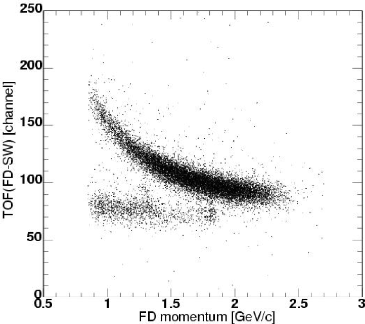
Figure 2: The TOF difference between particles detected in the FD and protons in SW scintillators versus the momentum of particles in the FD. Protons detected in the FD produce the upper curved band whereas the TOF of pions is almost independent of the momentum.

In contrast to the PD, the two layers of scintillators used in the FD are placed very close to each other and, in order to identify protons, the TOF difference between the SW and FD scintillators had to be combined with the measurement of the momentum of particles detected in the FD, as shown in Fig. 2. Coincident protons were selected in the PD as described above and their momenta reconstructed to make a correction for the different trajectory lengths. In the momentum range of interest, which is below 1.8 GeV/c, the proton and pion bands are well separated except in the vicinity of 1.75 GeV/c. Here the numbers of pions are strongly enhanced by the proton–neutron final state interaction in the $pp\rightarrow pn\pi^{+}$ reaction. However, if misidentified as protons, such pions will produce a peak in the $pp$ missing–mass distribution at 0.65 GeV/c² and 0.68 GeV/c² for 2.85 GeV/c and 2.95 GeV/c, respectively. This allows the possibility to control the proton selection also in the overlap region of Fig. 2. The total loss of protons as a result of the selection was estimated to be $(7\pm 2)\%$.

To determine the efficiency of a single FD MWPC, the trajectory of a particle has been found using only information from the other two MWPCs. Having calculated the point at which the trajectory intersects the sensitive plane of the MWPC under investigation, the presence of a valid neighbouring cluster has been checked to satisfy all requirements applied in the track–finding algorithm Dymov . This procedure resulted in an efficiency map for each of the sensitive planes, which was subsequently used to introduce the efficiency correction on an event–by–event basis. Only one sensitive plane among the seven involved in the FD track reconstruction was found to have an inhomogeneous distribution of efficiency in approximately $30\%$ of its sensitive area, with an average value of $88\%$. All the others had homogeneous maps with average efficiencies above $96\%$.

The influence of the total efficiency corrections on the missing–mass distributions has been checked using the ratio of corrected to uncorrected spectra, which was found to be constant to within experimental errors. The average efficiency was about 75%.

3 Selection of $\mathsf{pp\to pp\omega}$ events

Histograms representing the overall missing–mass ($m_{X}$) distributions from the $pp\rightarrow ppX$ reaction at the two beam momenta are shown in Fig. 3.

Figure 3: The missing–mass distributions of the $pp\rightarrow ppX$ reaction measured (a) at 2.85 GeV/c and (b) at 2.95 GeV/c. There is clear evidence for peaks corresponding to the production of both the $\eta$ and $\omega$ (indicated by arrows) but sitting on a large multipion background.

Both spectra show similar features. There is a sharp rise from the kinematic limit on the right due to the multiparticle phase space, whereas the more gentle fall to the left is mainly a reflection of the ANKE acceptance. Sitting on top of this multipion background there are small peaks due to the production of the $\eta$– and $\omega$–mesons. Evidence for the $pp\rightarrow pp\pi^{0}$ reaction was also found below 0.4 GeV/c², but the pion peak has a large width because the effects of momentum uncertainties are significantly amplified in this region of large excess energies.

The accuracy of the missing–mass reconstruction was verified using the $pp\rightarrow{}pp\eta$ and the $pp\rightarrow{}pn\pi^{+}$ reactions, with the results being presented in Table 1.

Table 1: Missing masses of various reactions in MeV/c² for the two beam momenta.

$m_{X}$	2.85 GeV/c	2.95 GeV/c
$m_{n}(\pi^{+}_{PD},p_{F\!D})$	$939.3\pm 0.1$	$939.6\pm 0.1$
$m_{n}(p_{PD},\pi^{+}_{F\!D})$	$939.2\pm 0.2$	$939.8\pm 0.2$
$m_{\eta}(p_{PD},p_{F\!D})$	$547.8\pm 0.1$	$547.4\pm 0.1$
$m_{\omega}(p_{PD},p_{F\!D})$	$782.3\pm 0.4$	$782.7\pm 0.4$

In the pion case, the neutron mass was reconstructed in both possible variants, either when the proton was found in the FD and the pion in the PD or vice versa. Given the good agreement achieved in these cases, one should expect to find the $\omega$ peak at its nominal position. However, in the vicinity of the $\omega$ mass, the large background from multipion production is strongly peaked, due to the specific acceptance of the ANKE magnetic spectrometer, and the challenge is to extract the number of $pp\rightarrow{}pp\omega$ events. To select the $\omega$ signal from Fig. 3, a kinematical transformation of the experimental missing–mass distribution from one beam momentum to the other was applied, as illustrated in Fig. 4. This approach was proposed and successfully used in the study of $\omega$ production at lower excess energies with the SPESIII spectrometer SPES . It avoids the need to construct specific models for a background that is unlikely to follow phase space. The scheme involves an event–by–event Lorentz transformation of the momenta of both final protons from the laboratory system where they were actually measured to the laboratory system at another beam momentum. If the phase space of the multipion production processes is much larger than the experimental acceptance, the shape of the missing–mass distribution related to this background is expected to be fixed by the acceptance and to remain the same in both systems. On the other hand, a peak corresponding to the production of a single meson is shifted by approximately the difference in centre–of–mass energies, as seen clearly for $\eta$ production in Fig. 4. The solid histogram in the top panel of this figure represents the missing–mass distribution actually measured at 2.85 GeV/c (see Fig. 3a). The dashed histogram represents the result of such a transformation of the missing–mass distribution obtained at the 2.95 GeV/c beam momentum (see Fig. 3b) to the 2.85 GeV/c. The transformed distribution is normalised by the ratio of the sums of events in the 0.6–0.7 GeV/c² range, which gives a factor of $1.054\pm 0.006$.

Figure 4: Upper frame: The missing–mass distribution of the $pp\rightarrow ppX$ reaction measured at 2.85 GeV/c (solid line, Fig. 3a) is shown together with the analogous distribution obtained at 2.95 GeV/c (Fig. 3b) and kinematically transformed to the 2.85 GeV/c (dashed line), as described in the text. Lower frame: The bin–by–bin difference of these two distributions is represented by points. The solid lines show simulations of the $pp\rightarrow{}pp\eta$ and $pp\rightarrow{}pp\omega$ reactions convoluted with acceptance. The widths of the peaks, which are strongly influenced by effects of momentum reconstruction, are very well reproduced.

The difference between the actual and transformed distributions, shown by points in the lower frame of Fig. 4, demonstrates clear positive (negative) peaks corresponding to $\eta$ and $\omega$ production in the actual (transformed) cases. These peaks are in a good agreement with the simulations of these reactions (solid line). The missing–mass distributions simulated at 2.95 GeV/c were transformed to 2.85 GeV/c and subtracted in the same way as the experimental one. The $\eta$ and $\omega$ experimental widths arise mainly from the uncertainties in the momentum reconstruction. Finally, the difference spectrum for $m_{X}>0.65\,$MeV/c² was fitted by two Gaussian functions in order to extract the number of events in the $\omega$ peak, its statistical uncertainty, and the position of the peak at $Q=60\,$MeV (see Table 1).

The same procedure was applied to extract the total number of $\omega$-mesons detected at $Q=92$ MeV. In this case the missing–mass distribution measured at a beam momentum of 2.85 GeV/c was transformed to 2.95 GeV/c.

However, the good agreement found for the shapes of the background spectra in the region between the $\eta$ and $\omega$ peaks does not necessarily prove that the same is true also underneath the $\omega$ peaks. In principle, up to six pions might be produced at our energies, but only those with two and three pions in the final state have phase spaces much larger than the ANKE acceptance. Although the total cross sections for the production of four or more pions are at least an order of magnitude smaller, they have larger acceptances in ANKE and populate missing masses mostly near the kinematical limit.

The direct way of verifying the shape of the background under the $\omega$ peak, by interpolating between two transformed distributions measured above and below the given excess energy, is not possible here since data were taken at only two energies. An attempt to describe the multipion background with the help of phase–space simulations, adjusting the relative contribution of reactions with different number of pions, was also undertaken. However, no set of parameters could simultaneously provide an appropriate reproduction of the background shape in different parts of the acceptance, probably due to the neglect of all resonance effects. We have therefore used the following procedure to evaluate the possible variation in the shape near the kinematical limit in the missing mass.

Figure 5: The missing–mass distribution of the $pp\rightarrow{}ppX$ reaction obtained at 2.85 GeV/c within a restricted part of the total acceptance (closed circles) is shown together with the corresponding distribution kinematically transformed from the 2.95 GeV/c to 2.85 GeV/c (crosses). The thick solid line represents a fit to the distribution at 2.85 GeV/c while the thin one shows the background function under the $\omega$ peak found in this case. The same fit procedure was applied to the transformed distribution and the resulting background function shown by the dashed line.

Due to the characteristics of the ANKE installation, the shape of background varies across the total spectrometer acceptance. Using this feature, an acceptance range was found where the shape of background could be directly established from the fit procedure. The results from this are shown in Fig. 5. Both the measured and the transformed distributions were then separately fitted, using the same function to describe the background, together with a Gaussian function for the $\omega$ peak. The transformed distribution in Fig. 5 was scaled by $1.086\pm 0.011$, i.e. the ratio of the integrals under the background functions obtained in this way. The ratio of the background functions is not quite constant over the range but, apart from the 5–7 MeV/c² interval next to the kinematical limit, the deviation from unity is rather small. The difference between the background functions observed near the maximum of the distribution does not exceed $5\%$, changing sign in vicinity of 0.75 GeV/c², and staying at the $2\%$ level at smaller masses. Since the accuracy of the fit is similar to these deviations, a variation of $3\%$ has been considered as a measure of the systematics when the number of events under the $\omega$ peak could be determined only from the difference of experimental distributions at different energies.

The total numbers of $\omega$-mesons deduced from fits to the distribution at 2.85 GeV/c shown in the lower frame of Fig. 4, and the analogous one at 2.95 GeV/c, were found to be:

$5560\pm 540(\textrm{stat.})\pm 660(\textrm{syst.})$ at $Q=60$ MeV,

$5360\pm 480(\textrm{stat.})\pm 720(\textrm{syst.})$ at $Q=92$ MeV.

The large statistical errors are the result of the subtraction procedure as well as the need to describe two peaks of opposite sign situated close to each other.

4 Analysis of differential distributions

The restriction on the particle momenta registered in the PD leads to some mismatch in the FD and the PD momentum ranges and this in turn results in a limitation on the $pp\rightarrow{}pp\omega$ phase space available within the ANKE acceptance. The acceptance corrections can therefore not be done in a model–independent way and some assumptions have to be made on the differential distributions to determine the total cross section. To test the validity of these assumptions, we have compared a number of one–dimensional $pp\to{}pp\omega$ experimental distributions with the results of simulations. The following observables have been considered:

• The excitation energy in the two–proton rest frame:
  $\varepsilon_{pp}=M_{\rm inv}(p,p)-2m_{p}$.

• The excitation energy of the $\omega$-meson and the proton detected in the PD: $\varepsilon_{\omega p}=M_{\rm inv}(\omega,p)-m_{p}-m_{\omega}$.
  In this case, the total range of the Dalitz plot projection could be covered due to the large FD momentum acceptance. The range of the other projection, where the proton was detected in the PD, was less than 40 MeV and 75 MeV at excess energies of 60 MeV and 92 MeV, respectively.

• The angle of the $\omega$-meson with respect to the beam direction in the overall centre–of–mass system: $\cos\Theta_{\rm cm}$.

• The angle of a proton momentum $\vec{q}$ with respect to the beam direction in the $pp$ rest frame: $\cos\Theta_{pp}$.

• The angle of $\vec{q}$ with respect to the momentum of the $\omega$-meson in the $pp$ rest frame: $\cos\Psi_{pp}$.

The number of $\omega$-mesons in each bin of such a distribution was determined from the corresponding missing–mass spectrum using approaches that depended slightly on the shape of background and the position of the $\omega$ peak relative to the upper edge of the spectrum.

• When, as in Fig. 5, the shape of the background could be clearly established, a preference was given to the fit procedure described above. The missing–mass transformation was used to check that the description of the background below the $\omega$ peaks was reasonable. It was found that the normalisation factor of the transformed missing–mass distribution to the measured one is not constant, but may vary by up to $7\%$. Therefore, this factor had to be determined for each bin.

• In cases where the fit procedure could only be applied at a single excess energy, generally at 92 MeV, the background function for the corresponding transformed distribution was obtained. A simple scaling of this function was then allowed which, together with a Gaussian $\omega$ peak, was used to fit the distribution measured at the other excess energy. The scaling parameter thus obtained was used for the normalisation of the transformed distribution to the measured one. The number of $\omega$-mesons obtained as a result of the fit was verified using the difference of distributions of the type shown in Fig. 4. This procedure was also applied at $\varepsilon_{pp}>60\,$MeV, where the distributions transformed from 2.85 GeV/c to 2.95 GeV/c no longer contained the $\omega$ peak.

• The scenarios outlined above describe more than $80\%$ of our data. For the remainder, the transformed distribution was normalised by the ratio of the numbers determined after excluding the range covered by the actual and the transformed $\omega$–peaks from each of the spectra. It was verified that the sum of background events under the actual $\omega$–peak found in this and the previous two cases is equal within errors to the total number of background events shown in Fig. 4.

In all the cases, different assumptions regarding the background functions and/or different normalisation factors were tested in order to establish possible systematic errors, and these are incorporated into the vertical error bars on the points presented in Fig. 6.

The $pp\rightarrow{}pp\omega$ reaction was simulated at both excess energies using the PLUTO event generator PLUTO under different assumptions on the distribution of events over the total phase space of the reaction. Both protons were traced through the ANKE acceptance with the help of the GEANT3 package GEANT . To check the tracing procedure, the momentum and angular acceptances of all the scintillators, as well as their images in the MWPCs, have been evaluated and compared with the corresponding experimental ones. They were found to coincide to within the experimental errors. Finally, the total number of accepted events simulated at each excess energy was normalised to the corresponding total number of $\omega$-mesons obtained in the experiment.

Figure 6: The distributions of experimental (points) and simulated (lines) $\omega$-meson yields for different reaction observables at 60 MeV (left panels) and 92 MeV (right panels). The different simulations correspond to pure phase space PS (solid line), full FSI (dashed line), phase space distorted by an angular dependence in the $\Psi_{pp}$ variable (dash–dotted line), and partial FSI with the distorted angular distribution (dotted line), as described in the text. The corresponding total cross sections are given in Table 2.

The solid lines in the Fig. 6 demonstrate the distributions expected in the case of a three–body phase space (PS), whereas those shown by dashed lines take into account the final state interaction (FSI) between the two protons. Following Goldberger and Watson Gold , the FSI enhancement factor $I(q)$ was calculated using the Jost function $J(q)$:

$$I(q)=|J(q)|^{-2}=\left(\frac{q^{2}+\beta^{2}}{q^{2}+\alpha^{2}}\right)\>,$$ (4.1)

where $q=|\vec{q}|$ is the magnitude of the proton momentum in the $pp$ rest frame. On the basis of the $pp$ scattering length and effective range we took $\alpha=-20.5\,$MeV/c, $\beta=167\,$MeV/c.

Figure 7: Missing–mass distribution of the $pp\rightarrow{}ppX$ reactions obtained at $Q=92\,$MeV in the $10<\varepsilon_{pp}<30\,$MeV range (closed circles) is shown together with the corresponding transformed distribution (crosses). The thick solid line represents the fit result for the measured spectrum. The dashed and dashed–dotted lines show two extreme cases of the background behaviour. The maximum systematic error was established to be $25\%$.

Due to the selection of one proton in the FD and the other in the PD, the experiment had no acceptance for $\varepsilon_{pp}<10\,$MeV. As a consequence, and as shown by the left panels of Fig. 6, the distributions at $Q=60\,$MeV cannot distinguish between the pure PS and FSI models. However, at $Q=92\,$MeV, the experimental yield in the $10<\varepsilon_{pp}<30\,$MeV range is about a factor of two lower than that expected on the basis of the FSI model. It must be noted that the yield in this bin can be determined very reliably, as shown by the corresponding missing–mass spectrum in Fig. 7. The fit procedure applied to the missing–mass distribution at $Q=92\,$MeV would give an even smaller yield than that found taking into account the behavior of the transformed spectrum under the peak. Different background functions were tested, but none of them could increase the yield by more than $25\%$ assuming a smooth shape under the $\omega$ peak.

The low experimental yield at $Q=92\,$MeV for $\varepsilon_{pp}<30\,$MeV is similar to that observed in the analogous $pp\to{}pp\eta$ reaction at 74 MeV, where the effects of the FSI in the $pp$ system were found to be very small Pauly . This may be an indication that the $pp$ $S$–wave is weak and that higher $pp$ partial waves are important. In this connection it should be noted that the distributions in the proton angles in the $pp$ rest frame, especially, $\Psi_{pp}$, would allow some anisotropy. This contrasts with the yield distributions in the meson centre–of–mass angle, which correspond quite well to an isotropic $\textrm{d}\sigma/\textrm{d}\cos\Theta_{\rm cm}$ at both the excess energies. The TOF collaboration reported a similar behaviour TOF .

The dash–dotted lines in Fig. 6 were calculated assuming that the three–body phase space is modified by a factor

$$1+a\,P_{2}(\cos\Psi_{pp})\,,$$ (4.2)

where $P_{2}(\cos\Psi_{pp})$ is a Legendre polynomial, and $a=0.6$ at $Q=92\,$MeV. It is interesting that this assumption gives a better description of the data, not only for the $\cos\Psi_{pp}$ distribution, but also for that of $\cos\Theta_{\rm cm}$ in the $-0.9$ region. At $Q=60\,$MeV we would expect any anisotropy to be smaller. The case of $a=0.2$ was tested but, for all the observables other than $\cos\Psi_{pp}$, the results differ little from the PS case.

Although the introduction of an angular dependence through eq. (4.2) provides a quite adequate description of all the distributions, with no need for the $S$–wave FSI, it seems unlikely that this would be suppressed completely. To test some of the possibilities, we have adjusted the contribution of the FSI to provide a slightly better description of the data; the results shown by dotted lines in Fig. 6 were achieved by decreasing the FSI enhancement by factors of $0.8$ and $0.4$ at $Q=60\,$MeV and 92 MeV, respectively. The values of the total cross sections obtained on the basis of these various assumptions are presented in Table 2. Other variants, including allowing some dependence on $\Theta_{pp}$, invariably give results that lie within the ranges shown in the table.

Table 2: Total cross sections for different models. The form of the FSI factor is given in eq. (4.1) and that of the assumed angular dependence in eq. (4.2).

	$Q=60\,$MeV	$Q=92\,$MeV
Model	$a=0.2$	$a=0.6$
	$k=0.8$	$k=0.4$
PS	5.0 $\mu$b	10.8 $\mu$b
PS + FSI(100%)	7.1 $\mu$b	14.3 $\mu$b
PS + $a\,P_{2}(\cos\Psi_{pp})$	4.8 $\mu$b	10.4 $\,\mu$b
PS + $k\times$FSI + $a\,P_{2}(\cos\Psi_{pp})$	6.6 $\mu$b	12.0 $\mu$b

5 Results and Discussion

Combining the results of all the variants that can hardly be distinguished within the errors, we find total cross sections lying in the ranges $4.8-7.1\mu$b at $Q=60\,$MeV and $10.4-14.3\mu$b at 92 MeV, respectively. The highest values are achieved with the rather unrealistic pure FSI model and so we take rather the last two lines of Table 2 as an indication of the model–dependence of the results. These give

$\sigma(Q=60\,$MeV$)=$	$\,\phantom{1}(5.7\pm 0.6_{\rm stat}\pm 0.8_{\rm syst}\pm 0.9_{\rm mod})\>\mu$b,
$\sigma(Q=92\,$MeV$)=$	$\,(11.2\pm 1.1_{\rm stat}\pm 1.7_{\rm syst}\pm 0.8_{\rm mod})\>\mu$b ,

where the first error represents the statistical uncertainty. The second figure stands for the total experimental systematic uncertainty, which includes contributions from the luminosity determination, the possible change of acceptance due to uncertainties in the detector positioning, but mainly the determination of the total number of $pp\omega$ events. These were all treated as independent errors. The final number is our estimate of the influence of the model on the acceptance calculation.

Figure 8: The energy dependence of the $pp\rightarrow{}pp\omega$ total cross section. Our two points (closed circles) are compared with earlier data from Refs. SPES (triangles), DISTO (square), and TOF (open circles). In all cases, systematic and statistical eros have been added in quadrature. The chain and dashed curves show respectively the normalised energy dependence of eq. (5.4) with and without smearing over the finite $\omega$ width. The solid line is a purely phenomenological interpolation of the whole data set given by eq. (5.3).

Our $pp\to{}pp\omega$ total cross sections are shown in Fig. 8 with vertical error bars estimated from the quadratic sum of both the systematic and statistical errors presented above. Also shown are the results of other experiments at low $Q$ SPES ; DISTO ; TOF . The 92 MeV value is slightly higher than that of TOF, though the error bars do overlap. With the possible exception of the highest SPESIII point, the results are consistent with a smooth energy dependence and a global fit to the whole data set yields

$$\log_{10}\sigma=-0.855+0.495\log_{10}Q+0.230\left(\log_{10}Q\right)^{2},$$ (5.3)

where $Q$ is measured in MeV and the cross section in $\mu$b. This is also shown in the figure.

In the SPESIII work SPES , the energy dependence of the total cross section was compared with a simplistic model, consisting only of three–body phase space but modified by the $S$–wave $pp$ FSI GFW . This leads to the analytic result:

$$\sigma(pp\to pp\omega)=C_{\omega}\>\left(\frac{Q/\epsilon}{1+\sqrt{1+Q/\epsilon}}\right)^{\!\!2},$$ (5.4)

where $\epsilon\approx 0.45$ MeV. However, at low excess energies it is important to smear this function over the width of the $\omega$–meson. Both these forms are shown in Fig. 8, with the value of $C_{\omega}=37\,$nb being chosen to fit the SPESIII points rather than those at higher energy. Although the $S$–wave assumption is clearly untenable at larger $Q$, the curves do suggest that $P$ or higher partial waves are important there and a good representation of the data can be obtained by adding a small amount of pure phase–space distribution to the FSI of eq. (5.4). While presenting a baseline against which one can judge the more refined theoretical models, this approach also shows that the finite–width effects are negligible in our energy domain.

The predictions of three microscopic models Nakayama ; Kampfer ; Fuchs are shown in Fig. 9. All of them are versions of a meson–exchange model, but with different emphasis on the role of the $N^{*}$ isobars. It should be noted that these calculations involve a large number of parameters, some of which have been adjusted in order to optimise agreement with the published data, including the differential distribution at 173 MeV TOF .

Figure 9: Experimental data on the $pp\rightarrow{}pp\omega$ total cross section shown in Fig. 8 compared with the predictions from microscopic theoretical models shown by the chain (Nakayama ), solid (Kampfer ), and dashed (Fuchs ) curves.

In the early work of Tsushima and Nakayama Nakayama , nucleonic and mesonic current contributions were considered but the energy dependence of the total cross section is described better by the inclusion of effects of nucleon resonances, and it is that curve which is shown in Fig. 9. Nevertheless, this calculation still underestimates the SPESIII data by about a factor of two even though the finite $\omega$ width was taken into account. Despite neglecting this, and the initial state interaction, Kaptari and Kämpfer Kampfer got good agreement with the then available data without relying on any $N^{*}$ contribution. It was shown there that the effects of the $S$–wave FSI are particularly important, for without it a phase–space energy dependence of the $Q^{2}$ type is predicted. The Tübingen group Fuchs had extensive recourse to several nucleon resonances, especially the $N^{*}(1535)$, but the novel feature of their approach is the coupling to off–shell $\omega$–mesons, which is particularly important close to the reaction threshold. If this is correct then one would expect interesting effects when the $\omega$ is measured exclusively through its $e^{+}e^{-}$ decay mode Fuchs .

Having established the energy dependence of the total cross section for $pp\to{}pp\omega$, we are now in a position to investigate further the OZI rule in near–threshold production processes. If the $(\omega,\phi)$ mixing in the vector meson nonet were ideal, such that the $\phi$ were a pure $s\bar{s}$ state, then its three-pion decay would be forbidden by the OZI rule OZI . That it takes place at all is interpreted as an indication that the mixing is not quite ideal. Using the Gell-Mann–Okubo mass formulae, Lipkin Lipkin estimated that the ratio of coupling strengths of the $\phi$ and $\omega$ to non–strange hadrons should be

$$R_{\mathrm{OZI}}=4.2\,\times 10^{-3}\>.$$ (5.5)

It is therefore useful to evaluate the ratio of the $\phi$ and $\omega$ production cross sections in $pp$ collisions at the same value of the excess energy:

$$R_{\phi/\omega}\equiv\frac{\sigma(pp\to{}pp\phi)}{\sigma(pp\to pp\omega)}\,\cdot$$ (5.6)

Taking the recent measurement Hartmann of the total cross section for $\phi$ production in $pp$ collisions at $Q=18.5$, 34.5, and 75.9 MeV in conjunction with the global fit of eq. (5.3) to the data set of Fig. 8, we find at these energies $R_{\phi/\omega}=(3.1\pm 0.6)\times 10^{-2}$, $(3.0\pm 0.7)\times 10^{-2}$, and $(2.4\pm 0.7)\times 10^{-2}$, respectively, where all error bars have been compounded quadratically. Applying the same procedure to the $\phi$ point reported by the DISTO collaboration leads to $R_{\phi/\omega}=(2.2\pm 1.0)\times 10^{-2}$ at 83 MeV. The mean value of $R_{\phi/\omega}=(2.8\pm 0.4)\times 10^{-2}\approx 7\times R_{\mathrm{OZI}}$, is lower than that obtained in Ref. Hartmann because of the higher values for $\omega$ production that are now apparent in Fig. 8. Although not statistically significant, there are indications from these numbers that $R_{\phi/\omega}$ might decrease with rising $Q$ but, to test this, data would be needed on $\phi$ production at higher values of $Q$. However, it should be noted that such a slow decline had been predicted in model calculations. This arises there through the decreasing effect of the destructive interference between the nucleonic and mesonic contributions to $\omega$ production as the energy is raised Speth .

6 Conclusions

We have presented new measurements of the $pp\to{}pp\omega$ reaction at excess energies of 60 and 92 MeV. The SPESIII technique SPES of kinematically shifting the data at one energy to estimate the background at a neighbouring energy was successfully employed for differential as well as total spectra. In this way the small $\omega$ signal in the missing–mass distribution could be identified despite the large amount of multipion production. With the setup actually employed for studying this reaction at ANKE, the acceptance, especially at small $\varepsilon_{pp}$, was limited. A variety of assumptions were tested against one–dimensional spectra in order to assess the model–dependence of the total $\omega$ production cross section that we obtained in this way. This led to uncertainties that were comparable to the statistical and other systematic errors. The value for the total cross section at 92 MeV is a little higher than that found by the TOF group TOF , but our two points join smoothly with the results of other experiments. There is evidence from the anisotropic $pp$ angular distribution at 92 MeV that $P$ or higher $pp$ partial waves are significant at this energy.

The new data allow us to extract the OZI ratio with greater confidence and smaller error bars than before. This results in a slightly smaller value of $R_{\phi/\omega}$ than previously quoted Hartmann , with possibly a hint of some energy dependence (but see also Ref. Sibirtsev ).

All three theoretical calculations considered Nakayama ; Kampfer ; Fuchs appeared after the broad outlines of the energy dependence of the total cross section had been determined experimentally and in some cases the model parameters were adjusted to reproduce this. Other experimental observables such as differential cross sections or decay angular distributions are needed to constrain the models more tightly and it is encouraging to note that analysing power results will soon be made available by the COSY–TOF collaboration Brinkmann . Since good data exist on $pn\to d\phi$ at low energies Yoshi , further data on $\omega$ production with a neutron target would be particularly helpful pndomega .

The WASA at COSY facility will soon become operational WASA . The production of the $\omega$ in $pp$ collisions could then be investigated, with larger geometrical acceptance and lower background, via the detection of the $\omega\to\pi^{0}\gamma$ decay ($BR\approx 9\%$) and the reconstruction of its invariant mass. Such an approach would also have the advantage of leading to a determination of the tensor polarisation of the $\omega$, a quantity which is very sensitive to the presence of higher partial waves. A similar sensitivity also exists in the spin–spin correlation in $\stackrel{{\scriptstyle\to}}{{p}}\stackrel{{\scriptstyle\to}}{{p}}\to pp\omega$, which could be measured at ANKE SPIN .