STAR Collaboration
Strange Particle Production in Collisions at = 200 GeV
Abstract
We present strange particle spectra and yields measured at mid-rapidity in GeV proton-proton () collisions at RHIC. We find that the previously observed universal transverse mass () scaling of hadron production in collisions seems to break down at higher and that there is a difference in the shape of the spectrum between baryons and mesons. We observe mid-rapidity anti-baryon to baryon ratios near unity for and baryons and no dependence of the ratio on transverse momentum, indicating that our data do not yet reach the quark-jet dominated region. We show the dependence of the mean transverse momentum () on measured charged particle multiplicity and on particle mass and infer that these trends are consistent with gluon-jet dominated particle production. The data are compared to previous measurements from CERN-SPS, ISR and FNAL experiments and to Leading Order (LO) and Next to Leading order (NLO) string fragmentation model predictions. We infer from these comparisons that the spectral shapes and particle yields from collisions at RHIC energies have large contributions from gluon jets rather than quark jets.
pacs:
25.75.-q, 25.75.Dw, 25.40.EpVersion 4.2
I Introduction
The production of particles in elementary proton-proton () collisions is thought to be governed by two mechanisms. Namely, soft, thermal-like processes which populate the low momentum part of the particle spectra (the so-called underlying event) and the hard parton-parton interaction process. In this scenario, the low transverse momentum () part of the spectrum is exponential in transverse mass () while fragmentation, in leading order models, introduces a power law tail at high . We investigate the validity of these assumptions at RHIC energies by studying the spectral shapes and the yields of identified strange hadron spectra from the lightest strange mesons () to the heavy, triply-strange baryon.
In this paper we report the results for transverse momentum spectra and mid-rapidity yields () of , , , , , , and measured by the STAR experiment during the 2001-2002 =200 GeV running at RHIC. After a brief introduction in Section II of the experimental setup and the conditions for this run, we provide a description of the event selection criteria and the efficiency of reconstructing the primary interaction vertex in Section III.1. Specific attention will be given to the complications introduced by more than one event occurring in the detector during readout, a condition referred to as “pile-up”. The details of strange particle reconstruction and the efficiency thereof will be discussed in Sections III.2, III.3, and III.4. In Section IV.1 we describe the final measured spectra and mid-rapidity yields. We also describe the functions that were used to parameterize the spectra in order to extrapolate the measurement to zero . We will show that the previously widely used power-law extrapolation for and collisions Bocquet96 does not yield the best results for the strange baryons and we will consider alternatives. Section IV.2 introduces the idea of transverse mass scaling (-scaling) and its applicability to our data. The measured anti-particle to particle ratios are presented in Section IV.3. Interesting trends of increasing mean transverse momentum, , with particle mass have been previously observed in collisions at ISR energies (20 63 GeV) Alper75 . Mean transverse momentum has also been found to increase with event multiplicity in collisions at SpS ( GeV) Bocquet96 and FNAL energies (300 GeV 1.8 TeV) E735 ; E735-2 . We will show the dependence of our measurements on both particle mass and event multiplicity in Section IV.4. We discuss the details of the experimental errors and then compare our results in Section V with several models that attempt to describe particle production in collisions via pQCD, string fragmentation, and mini-jets Gyulassy92 . We conclude in Section VI with a discussion of the major results and some remarks about future directions for the ongoing analyses.
II Experimental Setup
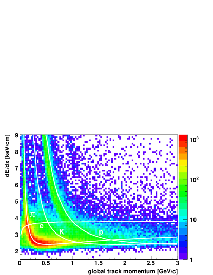
The data presented in this paper were collected with the STAR detector STAR . The primary detector sub-system used for these analyses is the large cylindrical Time Projection Chamber (TPC), which is able to track charged particles in the pseudo-rapidity range with full azimuthal coverage TPC . The TPC has 45 pad rows in the radial direction allowing a maximum of 45 hits to be located on a given charged particle track. A uniform magnetic field of 0.5 T is applied along the beam line by the surrounding solenoidal coils allowing the momentum of charged particles to be determined to within 2-7% depending on the transverse momentum of the particle. The field polarity was reversed once during the 2001-2002 run to allow for studies of systematic errors. The TPC tracking efficiency in collisions is greater than 90% for charged particles with MeV/ in the pseudorapidity region TPC . Particle identification may be achieved via measurements of energy loss due to specific ionization from charged particles passing through the TPC gas (). The , when plotted vs. rigidity separates the tracks into several bands which depend on the particle mass. A semi-empirical formula describing the variation of with rigidity is provided by the Bethe-Bloch equation Bichsel . An updated form, which accounts for the path length of a given particle through matter, has been given by Bichsel and provides a reasonable description of the band centers for the particles presented in this paper Bichsel . The Bichsel curves are shown in Figure 1.
The dataset analyzed in this paper consisted of minimally-biased events before cuts. After applying a cut requiring the location of the primary vertex to be within 50 cm of the center of the TPC along the beam axis, to limit acceptance variations, events remained. In all events, the detectors were triggered by requiring the simultaneous detection of at least one charged particle at forward rapidities () in Beam-Beam scintillating counters (BBCs) located at both ends of the TPC. This is referred to as a minimally biased trigger. The BBCs are sensitive only to the non-singly diffractive (NSD) part (30 mb) of the total inelastic cross-section (42 mb) ppSpecPaper ; STARBBCs . A more detailed description of STAR in general STAR and the complete details of the TPC in particular TPC can be found elsewhere.
III Analysis
III.1 Primary Vertex Finding and Event Selection
The position of the interaction vertex is calculated by considering only those tracks which can be matched to struck slats of the STAR central trigger barrel (CTB) CTB . The CTB is a scintillating detector coarsely segmented into 240 slats placed azimuthally around the outside of the STAR TPC at a radius of 2 m. It has a total pseudorapidity coverage of and has a fast response time of 10-60 ns, which is roughly one quarter of the time between beam bunch crossings (218 ns in the 2001-2002 run). Therefore, in approximately 95.6% of our collisions, only charged particles from the triggered event will produce signals in the CTB which ensures that the primary vertex is initiated with tracks from the triggered event only (note that, unlike the BBCs, the CTB itself is not used as a trigger detector for the event sample presented here). Furthermore, the primary vertex is assumed to be located somewhere along the known beam line. The z co-ordinate (along the beam) of the primary vertex is then determined by minimizing the of the distance of closest approach of the tracks to the primary vertex.
The RHIC beams were tuned so as to maximize the luminosity and, consequently, the number of collisions that can be recorded. The average RHIC luminosities, which varied from to , produce collisions more frequently (on the order of 2-200 kHz) than the TPC can be read out (100 Hz). During running, as many as five pile-up events can overlap (coming in the 39 s before or after an event trigger) in the volume of the TPC. Pile-up events come earlier or later than the event trigger and tracks from pile-up events may therefore be only partially reconstructed as track fragments. These track fragments from a pile-up event can distort the determination of the location of the primary interaction vertex as they do not point back to the vertex of the triggered event. To solve this, tracks that do not match to a struck CTB slat are not used in the determination of the primary vertex position. The remaining pile-up tracks, which match by chance to fired CTB slats, can then be removed with a reasonably restrictive (2-3 cm) analysis cut on a track’s distance of closest approach to the determined primary vertex.
Another problem faced in the event reconstruction is the observation that for many minimally-biased triggers no primary vertex is reconstructed. The problem is systematically worse for the low multiplicity events. Therefore, a correction must be applied to account for the events that are triggered on yet lost in the analyses due to an unreconstructed primary vertex.
The efficiency of the primary vertex finding software was investigated by generating Monte Carlo (MC) events, propagating the Monte Carlo produced particles through the STAR detector simulation (GEANT), then adding the resulting simulated signals into the abort-gap events. In an abort-gap event, the detectors are intentionally triggered when there are no protons in one or both of the beam bunches passing through the detector. Abort-gap events therefore contain background due to the interaction of beam particles with remnant gas in the beam pipe and may also contain background remaining in the TPC from collisions in the crossings of previous or subsequent beam bunches. Abort-gap events provide a realistic background environment in which to simulate the vertex finding process. The embedded simulated event is then passed through the full software chain and tracks are reconstructed. These events are then compared to the input from the MC events. A quantity , representing the difference along the z (beam) axis between the actual embedded MC primary vertex and the reconstructed primary vertex is defined as follows:
| (1) |
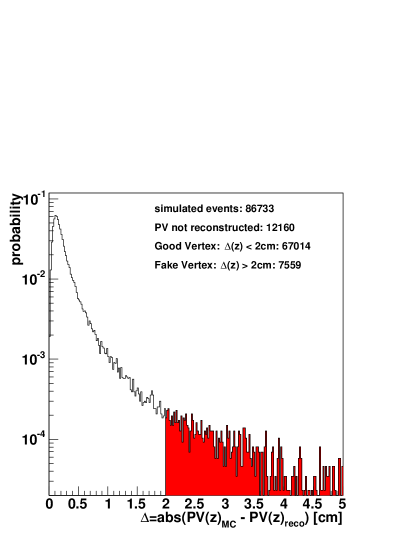
The probability distribution of is shown in Figure 2 for approximately 87,000 simulated events. We separate events where the software finds a vertex into two classes. An event with a good primary vertex is defined as having 2 cm, whereas a fake vertex event is one in which 2 cm. Whilst this limiting value is somewhat arbitrary, it does relate to offline cuts in our particle reconstruction that are sensitive to the accuracy of the found vertex.
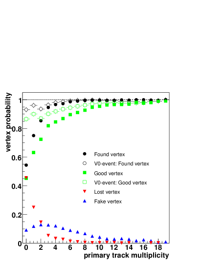
It was found that the probability of finding the primary vertex was strongly dependent on multiplicity. For the purposes of this study, “charged track multiplicity” is defined as being a count of tracks in the TPC that have at least 15 hits, at least 10 of which must be used in the track fit. After separating the raw charged track multiplicity distributions for each event class, i.e. lost vertex, fake vertex and good vertex, these distributions can be divided by the charged track multiplicity distribution of all events. This ratio then represents the probability for a certain event class to occur as a function of the measured charged track event multiplicity. Finally, the probabilities for each charged track multiplicity are mapped back to the corresponding primary track multiplicity, where “primary tracks” are those which satisfy the above requirements and additionally point back to within 3 cm of the primary vertex. The probabilities for each event class as a function of primary track multiplicity are shown in Figure 3. Whereas lost vertex events are monotonically decreasing with increasing multiplicity, fake vertex events are most probable when the event has 2 primary tracks. The open symbols in Figure 3 show the corresponding “found” and “good” probabilities for events that contained at least one strange particle decay candidate. Note that primary vertex finding is initiated with tracks pointing at fired slats of the CTB, as mentioned above. But all found tracks are allowed to contribute to the final vertex position. Therefore, on rare occasions and in low multiplicity events, a vertex may be found with no single track pointing back within 3 cm. These events will appear in Figure 3 as having a found (or fake) vertex but zero primary track multiplicity. The use of these probabilities to correct the strange particle yields and event counts as a function of multiplicity is described later.
III.2 Particle Identification
All the strange particles presented here, with the exception of the charged kaons, were identified from the topology of their weak decay products in the dominant channel:
| (2) |
| (3) |
| (4) |
| (5) |
The charged tracks of the daughters of neutral strange particle decays form a characteristic “V”-shaped topological pattern known as a “V0”. The V0 finding software pairs oppositely charged particle tracks to form V0 candidates. These candidates can then be further paired with a single charged track, referred to as the “bachelor” to form candidates for and decays. During the initial finding process, loose cuts are applied to partially reduce the background while maximizing the candidate pool. Once the candidate pool is assembled, a more stringent set of cuts is applied to maximize the signal-to-noise ratio and ensure the quality of the sample. The cuts are analysis dependent and are summarized in Table 1 for the and analyses and in Table 2 for the and analyses.
| Cut | and | |
|---|---|---|
| DCA of V0 to primary vertex | 2.0 cm | 2.0 cm |
| DCA of V0-daughters | 0.9 cm | 0.9 cm |
| N(hits) daughters | 14 | 14 |
| N() | 3 | 5 |
| Radial Decay Length | 2.0 cm | 2.0 cm |
| Parent Rapidity (y) | 0.5 | 0.5 |
| Cut | and | and |
|---|---|---|
| Hyperon Inv. Mass | 1321 5 MeV | 1672 5 MeV |
| Daughter Inv. Mass | 1115 5 MeV | 1115 5 MeV |
| N() bachelor | 5 | 3 |
| N() pos. daugh. | 5 | 3.5 |
| N() neg. daugh. | 5 | 3.5 |
| N(hits) bachelor | 14 | 14 |
| N(hits) pos. daugh. | 14 | 14 |
| N(hits) neg. daugh. | 14 | 14 |
| Parent Decay Length (lower) | 2.0 cm | 1.25 cm |
| Parent Decay Length (upper) | 20 cm | 30 cm |
| Daugh. V0 Decay Length (lower) | N/A | 0.5 cm |
| Daugh. V0 Decay Length (upper) | N/A | 30 cm |
| DCA of Parent to PVtx | N/A | 1.2 cm |
| DCA of Daughters | N/A | 0.8 cm |
| DCA of V0 Daughters | N/A | 0.8 cm |
| DCA of Bachelor to PVtx (lower) | N/A | 0.5 cm |
| DCA of Bachelor to PVtx (upper) | N/A | 30 cm |
| Parent Rapidity | 0.5 | 0.5 |
Several of these cuts require some further explanation. A correlation has been observed between the luminosity and the raw V0 multiplicity. This correlation is suggestive of pile-up events producing secondary V0s. The apparent path of the V0 parent particle (the or ) is extrapolated back towards the primary vertex. The distance of closest approach (DCA) of the V0 parent to the primary vertex is then determined. Secondary V0s from pile-up events do not point back well to the primary vertex of the triggered event and may therefore be removed via a cut on the DCA of the V0 parent to the primary vertex. Parent particles for secondary V0s may be charged and curve away from the primary vertex before decaying, causing the secondary V0 to also point back poorly. Therefore, this cut also removes some true secondary V0s.
Tracks in the TPC are occasionally broken into two or more segments that appear to be independent tracks to the V0 and finding software. In the majority of cases, this is due to tracks crossing the boundaries between sectors of the TPC pad plane. A cut requiring a minimum number of hits is applied to each of the decay daughter tracks to minimize the contamination from these track fragments.
Lastly, we define a variable N() to quantitatively measure the distance of a particular track to a certain particle band in vs. rigidity space STAR130Mult ; STAR130p-bar-p :
| (6) |
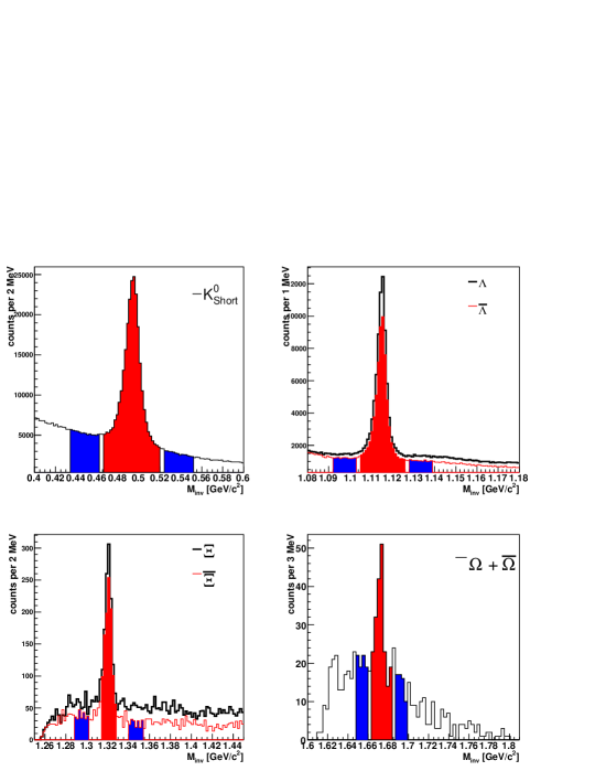
where R is the resolution (width in of the distribution of a given particle band, see Fig. 1) at the track’s momentum and is the number of hits used in the determination of the . Cutting on the N() of a given track helps to decrease the background even further by decreasing the contamination of the candidate pool due to misidentified tracks. This is particularly important for the analysis. The and analyses can tolerate more open cuts in favor of increased statistics. The invariant mass distributions for , , , and their corresponding antiparticles are shown in Figure 4.
The charged kaon decay reconstruction method is based on the fact that the four dominant decay channels (shown in relation 7) have the same pattern. The charged kaon decays into one or two neutral daughter(s) which are not detected and one charged daughter which is observed in the TPC.
| (7) |
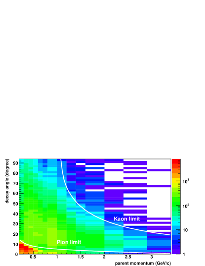
The decay topology corresponding to the above channels is known as a “kink”, as the track of the charged parent in the TPC appears to have a discontinuity at the point of the parent decay. The kink-finding software starts by looping over all tracks reconstructed in the TPC in the given event, looking for pairs of tracks which are compatible with the kink pattern described above. The first selection criterion is for the kaon decay vertex (the kink) to be found in a fiducial volume in the TPC. The TPC has an inner radius of 50 cm and an outer radius of 200 cm from the nominal beamline, but the fiducial volume is defined to have an inner radius of 133 cm and an outer radius of 179 cm. The fiducial volume is chosen to suppress background due to high track densities (inner cut) while allowing a reasonable track length for the determination of the daughter momentum (outer cut). This leads to a maximum number of hits for both the parent and daughter track in the fiducial volume. Additional cuts are applied to the found track pairs in order to select the kink candidates.
| Cut | (kinks) |
|---|---|
| Invariant mass | GeV/ |
| Kink angle | |
| Daughter mom. | 100 MeV/ |
| DCA/cm between Parent and Daughter |
and . See text and Figure 5 for further details.
For each kink found, a mass hypothesis is given to both the parent and daughter tracks (i.e. parent and daughter) and the pair invariant mass is calculated based on this hypothesis. A cut on the invariant mass ( in Table III) can then be applied. As charged pions decay with a branching ratio of approximately 100% into the same channel as the charged kaons, they will have the same track decay topology in the TPC. We therefore expect that the kink finding algorithm described above will include , , and as kink parent candidates. Therefore, several other cuts must be applied to further eliminate the pion background from the kaon decays in which we are interested. A summary of the applied cuts is given in Table 3.
In Figure 5 we show the regions excluded by the kink angle cut in Table 3. The cut is placed on the line marking the pion limit. In addition to the cuts listed in Table 3, a cut was applied to the specific energy loss to remove pion contamination below =500 MeV/ where the kaon and pion bands are clearly separated.
III.3 Signal Extraction
In order to extract the particle yield and , we build invariant mass distributions in several bins for each of the particle species except the charged kaons. The residual background in each bin is then subtracted through a method referred to here as “bin-counting”.
In the bin-counting method, three regions are defined in the invariant-mass distribution. The first, which is defined using the Gaussian signal width found by fitting the -integrated invariant-mass distribution with a linear function plus a Gaussian, is the region directly under the mass peak (, , and for the , , and respectively) which includes both signal and background (red or lightly shaded in Figure 4). For the and invariant mass distributions, the second and third regions (blue or dark shading in Figure 4) are defined to be the same total width as the signal region placed on either side ( away for and ) of the chosen signal region. For the , the second and third regions are each the size of the signal region and are placed away. In this method the background is implicitly taken to be linear under the mass peak. In bins where the background appears to deviate significantly from the linear approximation, a second degree polynomial fit is used to determine the background under the mass peak. This occurs mainly at low .
This procedure is carried-out in each transverse momentum bin and as a function of event multiplicity. The resulting spectrum is then corrected for vertex finding efficiency (Section III.4) as well as the particle specific efficiency and acceptance (Section III.1). The and spectra are further corrected for higher-mass feed-down as detailed in section III.5.
III.4 Particle Reconstruction Efficiencies
The number of reconstructed strange particles is less than the actual number produced in the collision due to the finite geometrical acceptance of the detector and the efficiency of the tracking and decay-finding software. Additionally, the quality cuts described in section III.2 reduce not only the combinatorial background but the raw signal as well.
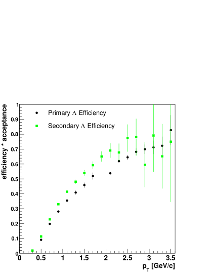
In order to determine the efficiency for each particle species as a function of transverse momentum, an embedding process, similar to that described in section III.1, is employed. In this process, a Monte Carlo generator is used to produce the particles of interest with a given transverse momentum distribution. The produced particles are propagated through the GEANT detector simulation and the resulting signals embedded into real events at the level of the detector response (pixel level). Using real events provides a realistic tracking and finding environment for evaluating the performance of the software. Only one simulated particle is embedded in any given event so as not to overly modify the tracking and finding environment. The embedded events are then processed with the full reconstruction software chain and the results compared with the input to determine the final correction factors for the transverse momentum spectra. Whether or not the event used for embedding already contained one or more strange particles is not a concern as only GEANT-tagged tracks are counted for the purpose of calculating efficiencies. The resulting total efficiencies (acceptance tracking, finding, and cut efficiencies) are plotted in Figure 6 for , , , , and . The correction is assumed to be constant over the measured rapidity region.
Finally, a correction needs to be applied to the raw particle yields due to low primary vertex efficiencies for low multiplicity events described in section III.1. The spectra were binned in multiplicity classes and for each class the particle yields were corrected using the probabilities corresponding to finding a good vertex in an event with at least a V0 candidate (open squares in Figure 3), thereby accounting for particles from lost and fake events. The overall event normalization is also corrected, using the numbers corresponding to the probability of finding a vertex (black filled circles in Figure 3), to account for the number of lost events.
| (kinks) | ||||||||||
| Error Source | dN/dy | dN/dy | dN/dy | dN/dy | dN/dy | |||||
| Cuts and Corrections (%) | 5.4 | 1.1 | 3.7 | 2.2 | 5.4 | 1.3 | 13 | 1.1 | 15 | 8.0 |
| Yield extraction and Fit function (%) | 4.9 | 3.7 | 1.5 | 1.2 | 6.3 | 4.7 | 30 | 5.6 | 20111The numbers for are for yield extraction only. The statistics do not allow a meaningful fit function study to be done for . | 3.0††footnotemark: |
| Normalization (%) | 4 | N/A | 4 | N/A | 4 | N/A | 4 | N/A | 4 | N/A |
III.5 Feed-down corrections
and baryons produce a as one of their decay products. In some cases, the daughter can be detected as if it were a primary particle. The result is a modification of the measured primary spectrum and an overestimation of the primary yield. The amount of contamination is unique to the cuts used to find the .
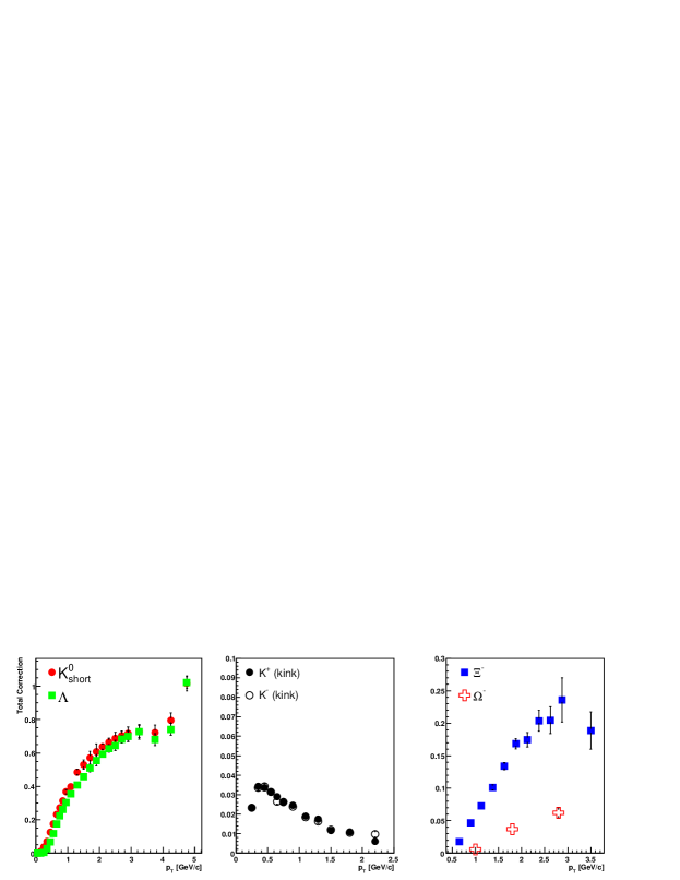
In order to correct this, Monte-Carlo simulations were performed and tuned to match the measured shape and yield of the spectrum presented in this paper. The shape and yield of the spectrum coming from decays can then be determined. The total correction factor (efficiency acceptance) was then calculated for both primary baryons and secondary baryons produced by embedded decays (see Figure 7). The correction factor is different for baryons coming from decays. Lastly, the secondary spectrum is multiplied by the correction factor for secondary baryons, divided by the primary correction factor, and the result is subtracted from the measured spectrum. The application of the correction factor is formalized in Equation 8,
| (8) |
where is the final feed-down corrected spectrum, is the non-feed-down corrected spectrum (corrected for efficiency and acceptance), is the secondary spectrum (determined from MC), and is the ratio of the secondary efficiency and acceptance correction to the primary efficiency and acceptance correction. The neutral has not been measured by our experiment and therefore, for the purposes of determining the feed-down correction, the yield is taken to be equal to the measured yield. Similarly, the yield is taken to be equal to the measured yield. By using Monte Carlo calculations, we determined that the finding efficiency for secondary particles was the same whether the comes from a charged or neutral . Therefore, the final feed-down correction is doubled to account for feed-down from decays.
III.6 Systematic Errors
Several sources of systematic errors were identified in the analyses. A summary of these errors and their estimated size is to be found in Table 4. A description of various sources of systematic error and their relative contribution is given below.
Cuts and Corrections: The offline cuts that are applied to minimize the residual backgrounds also help eliminate contamination from pile-up events. The cuts may be tightened to further reduce background or loosened to allow more signal and improved statistics at the cost of greater contamination. The final cuts are a compromise between these two extremes which aim to maximize the statistics for a given particle species while eliminating as much background as possible. The systematic errors from the cut-tuning provide an estimate for our sensitivity to changes in the various cuts.
This number includes the systematic errors from the embedding and vertex finding efficiency corrections. The and entry also accounts for the systematic errors from the feed-down correction.
Methods of Yield Extraction: In order to estimate the systematic error on the yield extraction in each bin, a second method of determining the yield in a given bin was used. In the second method, a combination of Gaussian plus a linear function is fit to the mass peak and background. The yield is then determined by subtracting the integral of the fitted linear function across the width of the signal peak from the sum of the bin content in the peak. In both methods, fitting and bin-counting, the background is assumed to be linear under the mass peak. A second degree polynomial fit is used in bins where this assumption is clearly invalid (mostly at low ). The two methods of extracting the yield may give different values due to the finite precision of the fitting method and fluctuations in the background in the bin-counting method. The difference in the two methods and any differences resulting from a deviation from the linear background assumption are taken into account by this systematic error.
The systematic error on the lowest /ndf functional parameterization of the spectra is also included in this row. It is estimated by comparing the yield and from the best /ndf functional parameterization with that from the second best /ndf functional form. The final numbers for the mid-rapidity yield and (in Tables 6 and 7) were determined for each particle using the fit with the smallest /ndf as shown in Table 5.
Normalization: The overall systematic error from the vertex and trigger efficiency affects only the particle yields and does not change the shape of the spectra. However, the vertex finding efficiency depends on the beam luminosity. The number quoted in this row is the level of fluctuation in the vertex finding efficiency with beam luminosity, 4%.
Conversion of our measurements to cross-sections must also account for an additional 7.3% uncertainty in the measured NSD trigger cross-section (261.9 mb) and for the 86% efficiency of the BBC trigger detectors.
IV Results
IV.1 Spectra
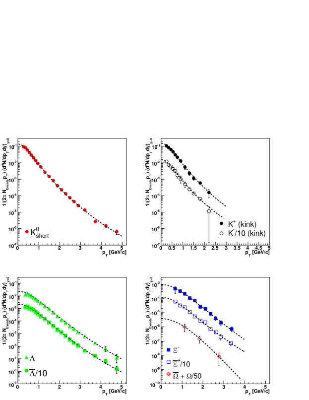
The fully corrected spectra for , , , , , and are shown in Figure 8. The measured spectra cover only a limited range in transverse momentum and therefore an appropriately parameterized function is needed to extrapolate into the unmeasured regions for the yield determination. In the past, exponential functions such as that given in Equation 9 have been used to extrapolate spectra from collisions to low transverse momentum while QCD-inspired power-law functions (see Equation 10) seem to provide a better description of the high (3 GeV/) region UA5 ; UA5:87 ; Bocquet96 ; Hagedorn . The coverage of the STAR detector for strange particles is large enough that a function which accounts for both the power-law component of the spectra and the low turnover becomes necessary to describe the data. A form that has been suggested is the Lévy function given by Equation 11 Wilk .
| (9) |
| (10) |
| (11) |
| Power-Law | Lévy | |||||
| Particle | ndf | ndf | ndf | |||
| 15 | 22 | 1.5 | 21 | 0.89 | 19 | |
| (kinks) | 3.1 | 11 | 7.0 | 10 | 0.40 | 9 |
| (kinks) | 9.4 | 11 | 5.0 | 10 | 0.30 | 9 |
| 4.5 | 22 | 3.3 | 21 | 0.81 | 18 | |
| 4.7 | 22 | 3.1 | 21 | 0.99 | 18 | |
| 0.84 | 9 | 1.4 | 8 | 0.76 | 8 | |
| 1.4 | 9 | 0.96 | 8 | 0.83 | 8 | |
| 0.13 | 1 | – | ||||
| Particle | dN/dy, | Stat. Err. | Sys. Err. |
|---|---|---|---|
| 0.134 | 0.003 | 0.011 | |
| (kinks) | 0.140 | 0.006 | 0.008 |
| (kinks) | 0.137 | 0.006 | 0.007 |
| 0.0436 | 0.0008 | 0.0040 | |
| 0.0398 | 0.0008 | 0.0037 | |
| (FD) | 0.0385 | 0.0007 | 0.0035 |
| (FD) | 0.0351 | 0.0007 | 0.0032 |
| 0.0026 | 0.0002 | 0.0009 | |
| 0.0029 | 0.0003 | 0.0010 | |
| 0.00034 | 0.00016 | 0.0001 |
| Particle | (GeV/) | Stat. Err. | Sys. Err. |
|---|---|---|---|
| 0.605 | 0.010 | 0.023 | |
| (kinks) | 0.592 | 0.071 | 0.014 |
| (kinks) | 0.605 | 0.072 | 0.014 |
| 0.775 | 0.014 | 0.038 | |
| 0.763 | 0.014 | 0.037 | |
| (FD) | 0.762 | 0.013 | 0.037 |
| (FD) | 0.750 | 0.013 | 0.037 |
| 0.924 | 0.120 | 0.053 | |
| 0.881 | 0.120 | 0.050 | |
| 1.08 | 0.29 | 0.09 |
| Particle | STAR dN/dy ( 0.5) | UA5 Yield | STAR Yield (scaled to UA5 y) |
|---|---|---|---|
| 0.134 0.011 | 0.73 0.18, | 0.626 0.051 | |
| 0.0834 0.0056 | N/A | 0.272 0.018 | |
| (FD) | 0.0736 0.0048 | 0.27 0.09, | 0.240 0.016 |
| 0.0055 0.0014 | , | 0.0223 0.0057 |
| Particle | STAR | UA5 |
|---|---|---|
| 0.61 0.02 | , | |
| 0.77 0.04 | , | |
| 0.903 0.13 | , |
where , , , , , , , and are fit parameters. Attempts were made to fit the spectra for our measured species with all three forms. A summary of the resulting ndf from each fit is given in Table 5 for each of the measured species. The mid-rapidity yields and mean transverse momenta quoted below were determined from the best fitting form which, for all species, was the Lévy form (Equation 11). The measured mid-rapidity yields and feed-down corrected yields are presented in Table 6. The measured mean transverse momenta are presented in Table 7.
Initially, we compare our measurement of neutral strange particles to similar experiments at this energy. The closest comparison can be made to the SS (Super Proton-Antiproton Synchrotron) experiments of UA1-UA5 using the beam. Only UA5 published strange particle measurements at =200 GeV UA5 ; UA5:87 , with others at =546 GeV UA5:546 and 900 GeV UA5 ; UA5:87 while UA1 published high statistics strange particle measurements at =630 GeV (Bocquet96 and references cited therein).
It is worth noting that the UA5 sample consisted of only 168 “manually sorted” candidates UA5 , whereas the STAR sample consists of fifty-eight thousand candidates.
Table 8 compares the values of and obtained from the STAR spectra to the published values from the UA5 experiment at SS UA5:87 measured with a larger rapidity interval. In the last column, the STAR data is scaled by a factor, obtained via Pythia pythia simulation, to account for the difference in rapidity coverage of the two experiments. UA5 measured with y2.5, with y2.0, and with y3.0. STAR measures only in the region y0.5. The STAR scaled yields are found to be in agreement with the measurement from UA5 and have greatly improved on the precision.
Table 9 compares the of the two experiments. It was verified, using Pythia, that the dependence of on the different rapidity intervals between STAR and UA5 is small, i.e. 2-3%. Therefore, the STAR measurement is compared to UA5 without further scaling and is found to have improved on the precision.
IV.2 Transverse Mass Scaling
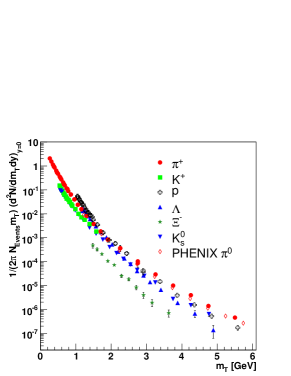
It has been noted previously that the identified particle spectra from collisions at ISR energies ISR75 ; ISR81 seem to sample an approximately universal curve when plotted versus transverse mass Wong , an effect termed “-scaling”. More recently, data from heavy-ion collisions at RHIC have been shown to scale in transverse mass over the measured range available Schaffner-Bielich02 . Transverse mass spectra from identified hadrons at =540 GeV and 630 GeV collisions at SpS have also been shown to exhibit the same behavior up to at least 2.5 GeV Schaffner-Bielich02 . The degree to which -scaling is applicable and the resulting scaling factors have been used to argue for the presence of a gluon-saturated state (color-glass condensate) in heavy-ion collisions at RHIC energies Schaffner-BielichCGC02 , though no such interpretation is applied to or collisions. Little discussion of the similarity of the results between and A+A has been provided. In Figure 9(a) we present the , , and spectra together with their antiparticles and with spectra for , K, and p from previously published STAR results at =200 GeV STAR-pi-k-p ; STAR-TOF ; STAR-rDEDX . The PHENIX spectrum from collisions at the same energy is also shown phenix-pi0 .
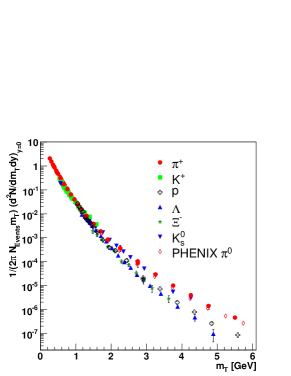
It is clear from Figure 9(a) that while the spectra appear to have qualitatively similar shapes, the yields are quite different. Nevertheless, the shape similarities encourage us to find a set of scaling factors that would bring the spectra onto a single curve. Figure 9(b) shows the result of scaling with the set of factors shown in Table 10. These factors were chosen so as to match the , K, and p spectra at an of 1 GeV. The higher mass spectra are then scaled to match the , K, and p spectra in their respective regions of overlap.
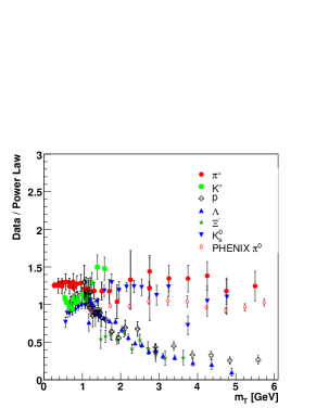
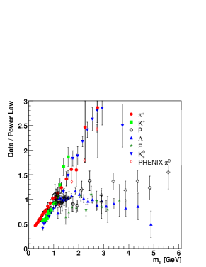
While the low- region seems to show reasonable agreement between all the measured species the region above 2 GeV shows an interesting new effect. The meson spectra appear to be harder than the baryon spectra with as much as an order of magnitude difference developing by 4.5 GeV in . In order to quantify the degree of agreement, a power-law function was fit to all the scaled meson and baryon spectra separately. The ratio of data to each fit was taken for each point in Figure 9(b). The data-to-fit ratio is shown for the meson fit in Figure 9(c) and the baryon fit in Figure 9(d).
This is the first time such a meson-baryon effect has been noticed in collisions. This effect is observable due to the high (and therefore high-) coverage of the strange particle and relativistic rise spectra STAR-rDEDX . The harder meson spectrum in the jet-like high- region may indicate that for a given jet energy, mesons are produced with higher transverse momentum than baryons. This effect would be a simple reflection of the fact that meson production from fragmentation requires only a (quark,anti-quark) pair while baryon production requires a (di-quark,anti-di-quark) pair. The difference between the baryon and meson curves appears to be increasing over our measured range, and it will be interesting to see, with greater statistics, what level of separation is achieved and whether or not the spectra eventually become parallel.
| K | p | ||||
|---|---|---|---|---|---|
| Scaling Factor | 1.0 | 2.0 | 0.6222Data from STAR-pi-k-p were scaled by 0.45 | 0.7 | 4.0 |
| Scaled at | 1.0 | 1.0 | 1.0 | 1.5 | 1.5 |
IV.3 Particle Ratios
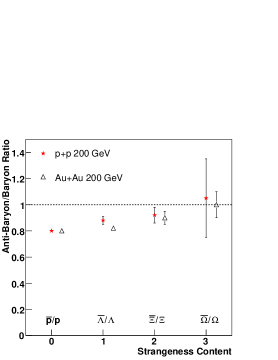
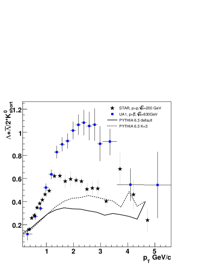
Figure 10(a) shows the mean anti-baryon/baryon ratios () as a function of strangeness content for and Au+Au at GeV HarrisSQM03 . The ratios rise slightly with increasing strangeness content and are consistent within errors with those from Au+Au collisions at the same center-of-mass energy. Although the ratios are not unity for the protons and baryons, the deviation from unity may be explained by different parton distributions for the light quarks HERA . This may be sufficient to explain the observed deviation from unity without having to invoke baryon number transport over five units of rapidity.
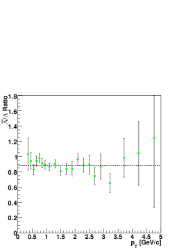
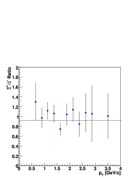
In the case of a quark jet, it is expected that there is a leading baryon as opposed to anti-baryon while there is no such distinction for a gluon jet. Therefore, making the assumption that at high the observed hadron production mechanisms are dominated by jet fragmentation, it is reasonable to expect that the ratio will drop with increasing . This has been predicted previously for calculations starting from as low as 2 GeV/ Xin-Nian . Figures 10(b) and 10(c) show the and ratios as a function of transverse momentum respectively. Although the errors shown in these figures are large, the ratios show no sign of decrease in the measured range. The dotted horizontal line in each figure is the error-weighted average over the measured range.
One conclusion that could be drawn from the ratios in Figure 10 is that particle production is not predominantly the result of quark-jet fragmentation over our measured range of .
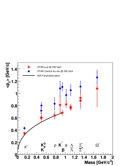
IV.4 Mean Transverse Momentum
One means of partially characterizing the spectra from collisions is through the determination and comparison of the mean transverse momentum. In Figure 11, the is shown for all particle species measured in both and central Au+Au collisions in STAR.
.
In total, twelve particles in both systems are presented, covering a mass range of approximately 1.5 GeV/. The solid line is an empirical curve proposed originally ISRcurve to describe the ISR ISR25GeV and FNAL FNAL data for , K , and p only, at = 25 GeV. It is interesting that it fits the STAR lower mass particles from at = 200 GeV remarkably well considering there is nearly an order of magnitude difference in collision energy. However, it is clear that a different parameterization would be needed to describe all of the STAR data. The dependence of the inverse slope parameter, T (and therefore of the ), on particle mass has previously been proposed to be due to an increasing contribution to the transverse momentum spectra from mini-jet production in and collisions Dumitru . The contribution is expected to be even greater for higher mass particles Gyu92_2 .
The available statistics allow a detailed study to be made. The mid-rapidity spectra can be binned according to eventwise charged particle multiplicity (uncorrected ) and the determined in each bin. We present in Figure 12 the dependence of on uncorrected charged particle multiplicity for , , , , and .
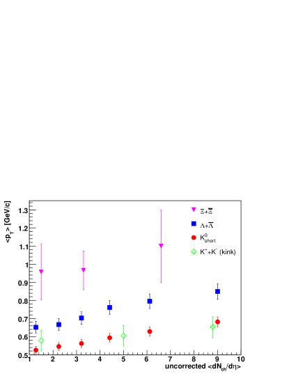
The scale difference is readily apparent but perhaps more interesting is the increasing trend of with event multiplicity. The increase in with multiplicity is faster for the than for the and charged kaons over the range from 2 to 6 in . The statistics available in the multiplicity-binned do not allow a proper constraint of the Lévy fit. The points for shown in Figure 12 were determined from the error-weighted mean of the measured distribution only. The present level of error on the measurement does not allow a strong conclusion to be drawn, though the trend with increasing mass is suggestive. This mass-ordering of the multiplicity dependence has been observed in previous measurements at three different energies E735 . In particular, the pions show little increase in when going from low to high multiplicity collisions E735 .
Models inspired by pQCD such as Pythia suggest that the number of produced mini-jets (and thereby the event multiplicity) is correlated with the hardness () of the collision. The effect of the mini-jets is to increase the multiplicity of the events and their fragmentation into hadrons will also produce harder spectra.
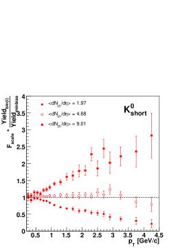
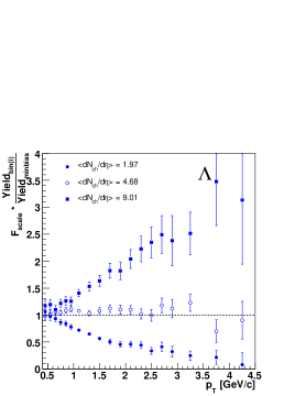
The spectral shape cannot be characterized by a single number. It is also possible to compare the multiplicity-binned spectra directly. We show in Figures 13(a) and 13(b) the ratio (Rpp) of the multiplicity-binned spectra to the multiplicity-integrated (minimum bias) spectra scaled by the mean multiplicity for each bin (see Equation 12) for and respectively.
| (12) |
where
| (13) |
The changes in incremental shape from one multiplicity bin to the next then become easier to see. The striking change in spectral shape going from the lowest to highest multiplicity bin is further evidence of the increasing contribution of hard processes (jets) to the high part of the spectra in high multiplicity events.
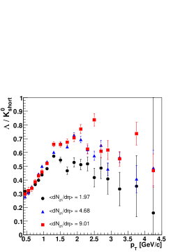
Figure 13(c) shows the / ratio as a function of in the various multiplicity bins. We see in all three bins that the shows a sharper increase with in the low ( 1.5 GeV/) part of the spectrum. Furthermore there seems to be a relative increase in the production in the intermediate GeV/ region.
V Model Comparisons
V.1 Comparison to PYTHIA (LO pQCD)
At the present time, the most ubiquitous model available for the description of hadron+hadron collisions is the Pythia event generator. Pythia was based on the Lund string fragmentation model string1 ; string2 but has been refined to include initial and final-state parton showers and many more hard processes. Pythia has been shown to be successful in the description of collisions of , and fixed target systems (see for example, ref. Field ).
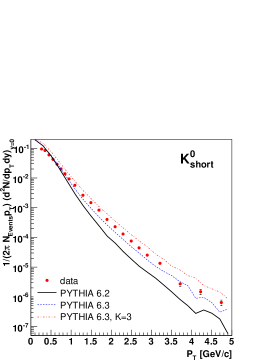
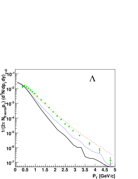
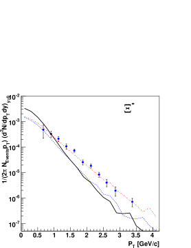
In this paper we have used Pythia v6.220 and v6.317 (using default settings with in-elastic cross-section (MSEL=1)) in order to simulate spectra for , and . These have then been compared with the measured data.
As shown in Figure 14, although there is some agreement at low , there are notable differences above 1.0 GeV/, where hard processes begin to dominate. Pythia v6.2 underestimates the yield by almost an order of magnitude at =3 GeV/. With the newer version 6.3, released in January 2005, these large discrepancies have been largely reconciled for but remain significant for and . This version includes a significantly modified description of the multiple parton scattering processes. The red dot-dashed lines in Figure 14 represent a simple tune that was done with Pythia 6.317 which will be described in more detail below.
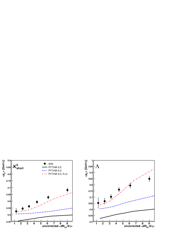
To try and understand the difference between Pythia and our results, we made comparisons of versus uncorrected charged multiplicity for and , as shown in Figure 15. As expected from the previous figure, version 6.2 fails to reproduce the minimum bias magnitude of . Although version 6.3 is capable of reproducing our minimum bias values of it clearly fails to reflect its increase with charged multiplicity, suggesting that further tuning is necessary.
In order to improve the agreement with our data we have made some simple changes to the Pythia default parameters. In particular, by increasing the K-factor to a value of 3 (set to 1 in the defaults) there is an enhancement of the particle yield at high in the model which allows it to better describe the data.
The K-factor, which represents a simple factorization of next-to-leading order processes (NLO) in the Pythia leading order (LO) calculation, is expected to be between 1.5–2 for most processes, such as Drell-Yan and heavy quark production kfactor at higher energies. Based on these measurements, a K-factor of 3 would signal a large NLO contribution, particularly for light quark production at RHIC energies. Intriguingly, a large K-factor has been estimated for the 200 GeV regime at RHIC based on the energy dependence of charged hadron spectra eskola-kfactor . So it seems that for light quark production at lower energies, NLO contributions are important and a comparison of our data to detailed pQCD based NLO calculations is more appropriate.
With the addition of this K-factor, we can see that the spectra for and in Figure 14 agree even better with the model, with the data falling slightly below the prediction. More importantly, the Pythia results of versus charged multiplicity, including the enhanced K-factor, are now in much better agreement with the data, as seen in Figure 15.
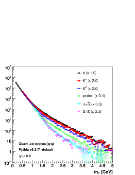
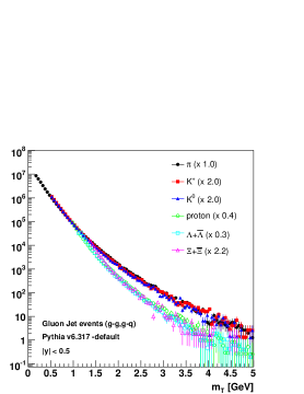
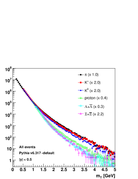
Figure 16 shows the results of separating Pythia events based on their final state parton content. Events where the final state is qq are labeled as containing “quark jets” while events with are labled as containing gluon jets. Figure 16(a) shows that events with only quark-jet final states seem to show a mass splitting in the high region while events whose final states contain jets from gluons (Figure 16(b)) show a shape difference between mesons and baryons with the meson spectra being harder than the baryon spectra. The shape difference is also apparent in Figure 16(c) which contains all final states including those with both quark and gluon jets. This shape difference could be simply related to the fact that a fragmentation process could impart more momentum to a produced meson than a produced baryon based on mass and energy arguments. This taken together with the results shown in Sections IV.2 and IV.3 indicates that above 2 GeV in transverse mass, the spectra contain significant contributions from gluon-jet fragmentation rather than quark-jet fragmentation.
In Figure 13(c) we showed the to ratio separated into multiplicity bins. Figure 17 shows the multiplicity integrated ratio compared with Pythia calculations using the default settings as well as a K-factor of 3. Here we see again the same shape difference between the and the that is seen for baryons and mesons in general in Figure 9(b) and in the p/ ratio STAR-rDEDX . Pythia is not able to reproduce the full magnitude of the effect in either ratio STAR-rDEDX . The to ratio shows a similar shape in GeV Au+Au collisions though the magnitude is larger and multiplicity-dependent Lamont06 . Also, measurements from UA1 at GeV indicate the magnitude may also be dependent on beam energy Bocquet96 .
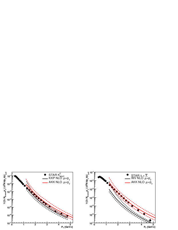
V.2 Comparison to NLO pQCD Calculations
In Figure 18 we compare the and spectra to NLO pQCD calculations including fragmentation functions for the from Kniehl, Kramer, and Pötter (KKP) KKP and a calculation by DeFlorian, Stratmann, and Vogelsang for the Vogelsang . The variations in show the theoretical uncertainty due to changes of the factorization and renormalization scale used. The factorization and renormalization scale allows one to weight the specific hard scattering contributions of the parton densities to the momentum spectrum. Although for the reasonable agreement is achieved between our data and the pQCD calculation, the comparison is much less favorable for the . Considering that good agreement was achieved for charged pion STAR-rDEDX and phenix-pi0 ; STAR-pi0 spectra and yields at the same energy, our comparison and the comparisons in STAR-rDEDX suggest that the region of agreement with NLO pQCD calculations may be particle species dependent. The baryons are more sensitive to the gluon and non-valence quark fragmentation function, which is less constrained at high values of the fractional momentum Bourrely Soffer .
Recently, the OPAL collaboration released new light quark flavor-tagged data which allows further constraint of the fragmentation functions OPAL . Albino-Kniehl-Kramer (AKK) show that these flavor separated fragmentation functions can describe our experimental data better AKK . However, in order to achieve this agreement, AKK fix the initial gluon to fragmentation function to that of the proton , and apply an additional scaling factor. They then check that this modified also works well in describing the SS data at =630 GeV. So, it appears that the STAR data is a better constraint for the high part of the gluon fragmentation function than the OPAL data. Similar conclusions have been drawn elsewhere with respect to the important role of RHIC energy collisions Fai . Recent studies of forward production also suggest that the region of agreement with NLO calculations extends as far out as 3.3 units in FPD .
V.3 Comparison to EPOS
Finally we compare our data to the version 1.02 of the EPOS model EPOSDetails . This model generates the majority of intermediate momentum particles by multiple parton interactions in the final state rather than fragmentation. The multi-parton cross section is enhanced through a space-like parton cascade in the incoming parton systems. The outgoing, time-like parton emission, is allowed to self-interact and to interact with the di-quark remnants. The interactions can be either elastic or inelastic. The overall result is a strong probability for multi-parton interactions before hadronization. The cascades are modeled through so-called parton ladders which also include multiple scattering contributions of the di-quark remnants from a hard parton scattering in a collision. Furthermore, by taking into account the soft pomeron interactions, the model is able to describe the spectra down to low . Finally, the inclusion of parton ladder splitting in asymmetric d+Au collisions yields a good description of the difference between and d+Au spectra in the same theoretical framework. Further details of the model can be found elsewhere EPOSDetails .
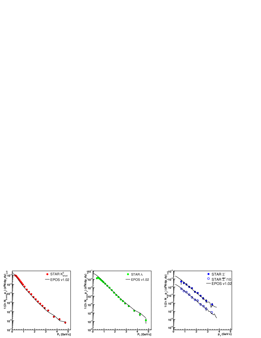
EPOS shows remarkable agreement with BRAHMS, PHENIX and STAR data for pion and kaon momentum spectra and in and d+Au collisions at both central and forward rapidities (STAR-rDEDX ; EPOS-RHIC ; EPOSDetails and references therein). Figure 19 shows that this trend also continues for the heavier strange particles at mid-rapidity. The agreement in collisions in the measured region is largely due to a strong soft component from string fragmentation in the parton ladder formalism. Remnant and hard fragmentation contributions are almost negligible at these moderate momenta. The soft contribution dominates the kaon spectrum out to 1 GeV/ and the spectrum out to 3 GeV/. As the momentum differences between (di-quark,anti-di-quark) and (quark,anti-quark) string splitting are taken into account, and the current mass difference between light and strange quarks is folded into the spectral shape, a comparison between the spectra exhibits a flow-like mass dependence.
The agreement with EPOS is better than even the best NLO calculations. A detailed discussion of the differences between EPOS and NLO calculations is beyond the scope of this paper, but it should be mentioned that the two models are, in certain aspects, complementary. More measurements of a) heavier particles and b) to much higher are needed in order to distinguish between the different production mechanisms. In summary, the data show the need for sizeable next-to-leading-order contributions or soft multi-parton interactions in order to describe strange particle production in collisions.
V.4 Statistical Model
The application of statistical methods to high energy hadron-hadron collisions has a long history dating back to Hagedorn in the 1960s Hagedorn65 ; Hagedorn68a ; Hagedorn68b . Since then statistical models have enjoyed much success in fitting data from relativistic heavy-ion collisions across a wide range of collision energies Hagedorn70 ; Siemens79 ; Mekjian82 ; Csernai86 ; Stocker86 ; Cleymans93 ; Rafelski02 ; PBM03 . The resulting parameters are interpreted in a thermodynamic sense, allowing a “true” temperature and several chemical potentials to be ascribed to the system. More recently, statistical descriptions have been applied to and collisions Becattini , and even Becattinie+e- , but it remains unclear as to how such models can successfully describe particle production and kinematics in systems of small volume and energy density compared to heavy-ion collisions.
It is important to note that a system does not have to be thermal on a macroscopic scale to follow statistical emission. For example, Bourrely and Soffer have recently shown that jet fragmentation can be parametrized with statistical distributions for the fragmentation functions and parton distribution functions Bourrely Soffer . In this picture, the apparently statistical nature of particle production observed in our data would be a simple reflection of the underlying statistical features of fragmentation. It is interesting to note that Biro and Mueller have shown that the folding of partonic power law spectra can produce exponential spectral shapes of observed hadrons in the intermediate region with no assumption of temperature or thermal equilibrium whatsoever Biro .
Another possibly related idea is that of phase space dominance in which all possible final state configurations (i.e. those that are consistent with the energy, momentum, and quantum numbers of the initial state) are populated with equal probability Hormuzdiar . The finite energy available in the collision allows many more final state configurations that contain low mass particles than high mass particles. The final state configurations containing high mass particles are therefore less likely to be observed not because they are less probable, but because there are fewer of them relative to the low mass configurations.
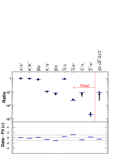
We include in this section the results of a canonical statistical model fit, using THERMUS THERMUS , to the STAR feed-down corrected ratios from collisions at =200 GeV. We used only the canonical formalism as it has been determined from a micro-canonical calculation that the volume of collision systems does not exceed 100 fm3 Liu04 . Previous results have shown that such a small volume invalidates the use of a grand-canonical treatment Liu03 . The canonical calculation involves only the temperature (T), baryon number (B), charge (Q), strangeness saturation factor (), and the radius. For this fit, B and Q were both held fixed at 2.0. The resulting parameters are presented in Table 11 and a graphical comparison is presented in Figure 20.
| Canonical Value | |
|---|---|
| T | 0.1680 0.0081 GeV |
| 2.000 (fixed) | |
| 2.000 (fixed) | |
| 0.548 0.052 | |
| 3.83 1.15 fm |
The interpretation of the fit parameters is difficult in the context of a collision where the system is not expected to thermalize and the volume is small. It is important to note that in a pure thermal model, all emitted particles would be expected to reflect the same temperature. Non-thermal effects such as flow would modify this result. In collisions, the particle spectra clearly show different slopes and those slopes are not in agreement with the T parameter that results from the statistical model fit to the particle ratios. As no flow is thought to be present in the system and the results of Section IV.2 support that conclusion, this result is a further indication of contributions to the particle spectra from non-thermal processes like mini-jets.
VI Summary and Conclusions
We have presented measurements of , , , , , , , and spectra and mid-rapidity yields from =200 GeV collisions in STAR. Corrections have been made for detector acceptance and efficiency as well as the multiplicity dependence of the primary vertex finding and, in the case of the and , feed-down from higher mass weak decays. It was found that the measured range of transverse momentum necessitates a functional form that accounts for the power-law like shape at high . We have used a Lévy function to fit the spectra and extrapolate to low .
The and mid-rapidity yields are in excellent agreement for all species with previous measurements at the same energy but with greatly improved precision. The anti-particle to particle ratios are flat with over the measured range for both the and and therefore show no sign of quark-jet dominance at high . The integrated ratios approach unity with increasing strangeness content. The anti-baryon to baryon ratios suggest that the mid-rapidity region at RHIC is almost baryon-free, at least in collisions. The amount of deviation from unity expected from differing parton distribution functions must first be determined before any claim of significant baryon number transport from beam rapidity to mid-rapidity can be made.
We have demonstrated the scaling of transverse mass spectra for low mesons and baryons onto a single curve to within 30% out to approximately 1.5 GeV in . Above 2 GeV the spectra show a clear difference in shape between mesons and baryons with the mesons being harder than the baryons. This is the first observation of a difference between baryon and meson spectra in collisions and is mainly due to the high (and therefore high ) coverage of the strange particles presented here. Pythia 6.3 seems to account for this effect and suggests it is mostly due to the dominance of gluon jets. More data are needed to determine the range of the effect.
The mean transverse momentum as a function of particle mass from both the and Au+Au systems has been compared. Both systems show a strong dependence of on particle mass. It is also worth noting that the mass-dependence of in the system seems to be independent of collision energy as the parameterization of the GeV ISR data seems to work well over the same range of measured masses at RHIC.
The dependence of on event multiplicity was also studied for each of the three species (and anti-particles). The shows a clear increase with event multiplicity for the and particles. There may be a mass-ordering to the increase as the baryons show a slightly faster increase with multiplicity than the , but the present level of error on the data does not allow a definite statement to be made.
The multiplicity-binned and spectra show a clear correlation between high multiplicity events and the high parts of the spectra. The spectral shapes for the and are observed to change with event multiplicity and the to ratio increases over the lower range and reaches higher values in the range above 1.5 GeV/ for larger multiplicites. This suggests that the high multiplicity events produce more hyperons relative to than the low multiplicity events.
Comparisons of our spectra with Pythia v6.221 show only poor agreement at best without adjustment of the default parameters. In the relatively high region (above 2 GeV/) there is nearly an order of magnitude difference between our data and the model calculation. The more recent Pythia 6.3 provides a much better description of our data though a K-factor of 3 is required to match the and spectra as well as the observed rate of increase of with multiplicity. NLO pQCD calculations with varied factorization scales are able to reproduce the high shape of our spectrum but not the spectrum. Previous calculations at the same energy have been able to match the spectra almost perfectly, which suggests that there may be a mass dependence to the level of agreement achievable with pQCD.
The EPOS model has previously provided excellent descriptions of the , , and proton spectra from both and d+Au collisions measured by BRAHMS, PHENIX, and STAR at mid-rapidity and forward rapidity. We have extended the comparison to strange and multi-strange mesons and baryons and have found the agreement between our data and the EPOS model to be at least as good as the best NLO calculations.
We have demostrated the ability of the statistical model to fit our data to a reasonable degree with three parameters. Interpretation of the resulting parameters in the traditional fashion is not possible as the colliding system is not considered to be thermalized. The T parameter does not agree with the slopes of the measured species and we conclude that this result suggests a significant contribution of non-thermal processes (such as mini-jets) to the particle spectra.
VII Acknowledgments
We would like to thank S. Albino, W. Vogelsang, and K. Werner for several illuminating discussions and for the calculations they have provided. We thank the RHIC Operations Group and RCF at BNL, and the NERSC Center at LBNL for their support. This work was supported in part by the HENP Divisions of the Office of Science of the U.S. DOE; the U.S. NSF; the BMBF of Germany; IN2P3, RA, RPL, and EMN of France; EPSRC of the United Kingdom; FAPESP of Brazil; the Russian Ministry of Science and Technology; the Ministry of Education and the NNSFC of China; IRP and GA of the Czech Republic, FOM of the Netherlands, DAE, DST, and CSIR of the Government of India; Swiss NSF; the Polish State Committee for Scientific Research; STAA of Slovakia, and the Korea Sci. & Eng. Foundation.
References
- (1) G. Bocquet et al., Phys. Lett. B 366, 441 (1996).
- (2) B. Alper et al. (British-Scandinavian Collaboration), Nucl. Phys. B 100, 237 (1975).
- (3) T. Alexopoulos et al. (E735 Collaboration), Phys. Rev. D48, 984 (1993).
- (4) T. Alexopoulos et al. (E735 Collaboration), Phys. Lett. B 336, 599 (1994).
- (5) X. N. Wang and M. Gyulassy, Phys. Lett. B 282, 466 (1992).
- (6) K. H. Ackermann et al. (STAR Collaboration), Nucl. Instrum. Meth. A 499, 624 (2003).
- (7) M. Anderson et al., Nucl. Instrum. Meth. A 499, 659 (2003).
- (8) H. Bichsel, Nucl. Instrum. Meth. A 562, 154 (2006); H. Bichsel, D. E. Groom, S. R. Klein, J. Phys. G 33, 258 (2006).
- (9) J. Adams et al. (STAR Collaboration), Phys. Rev. Lett. 92, 112301 (2004).
- (10) J. Adams et al. (STAR Collaboration), Phys. Rev. C70, 041901 (2004).
- (11) F. S. Bieser et al., Nucl. Instrum. Meth. A 499, 766 (2003).
- (12) C. Adler et al. (STAR Collaboration), Phys. Rev. Lett. 87, 262302 (2001).
- (13) C. Adler et al. (STAR Collaboration), Phys. Rev. Lett. 86, 4778 (2001); ibid 90, 119903 (2003).
- (14) R. E. Ansorge et al (UA5 Collaboration), Nucl. Phys. B 328, 36 (1989).
- (15) R. E. Ansorge et al (UA5 Collaboration), Phys. Lett. B 199, 311 (1987).
- (16) R. Hagedorn, Riv. Nuovo Cimento 6, n. 10, 1 (1984).
- (17) G. Wilk and Z. Włodarczyk, Phys. Rev. Lett. 84, 2770 (2000).
- (18) G. J. Alner et al. (UA5 Collaboration), Phys. Rep. 154, 247 (1987).
- (19) T. Sjöstrand et al., Computer Physics Commun. 135, 238 (2001).
- (20) B. Alper et al., Nucl. Phys. B 87, 19 (1975).
- (21) K. Alpgard et al., Phys. Lett. B 107, 310 (1981).
- (22) G. Gatoff and C. Y. Wong, Phys. Rev. D46, 997 (1992).
- (23) J. Schaffner-Bielich, D. Kharzeev, L. McLerran, and R. Venugopalan, nucl-th/0202054
- (24) J. Schaffner-Bielich, D. Kharzeev, L. McLerran, and R. Venugopalan, Nucl. Phys. A 705, 494 (2002).
- (25) J. Adams et al. (STAR Collaboration), Phys. Rev. Lett. 92, 112301 (2004).
- (26) J. Adams et al. (STAR Collaboration), Phys. Lett. B 616, 8 (2005).
- (27) J. Adams et al. (STAR Collaboration), Phys. Lett. B 637, 161 (2006).
- (28) S. S. Adler et al. (PHENIX collaboration), Phys. Rev. Lett. 91, 241803 (2003).
- (29) J. Harris, J. Phys. G 30, S613 (2004).
- (30) A. D. Martin, W. J. Stirling, and R. G. Roberts, Phys. Rev. D50, 6734 (1994).
- (31) X. N. Wang, Phys. Rev. C58, 2321 (1998).
- (32) M. Bourquin and J. M. Gaillard, Nucl. Phys. B 114, 334 (1976).
- (33) B. Alper et al., Nucl. Phys. B 114, 1 (1976).
- (34) J. W. Cronin et al. (Chicago-Princeton Group), Phys. Rev. D11, 3105 (1975).
- (35) A. Dumitru and C. Spieles, Phys. Lett. B 446, 326 (1999).
- (36) X. N. Wang and M. Gyulassy, Phys. Rev. D45, 844 (1992).
- (37) T. Sjöstrand, hep-ph/9508391; B. Andersson, G. Gustafson, G. Ingelman, and T. Sjöstrand, Phys. Rep. 97, 31 (1983).
- (38) B. Andersson, “The Lund Model” (Cambridge University Press, 1998); B. Andersson et al., hep-ph/0212122.
- (39) R. D. Field, Phys. Rev. D65, 094006 (2002); R. D. Field, hep-ph/0201192.
- (40) R. Vogt, Heavy Ion Phys. 17, 75 (2003).
- (41) K. Eskola and H. Honkanen, Nucl. Phys. A 713, 167 (2003).
- (42) J. Adams et al. (STAR Collaboration), nucl-ex/0601042, submitted to Phys. Rev. C.
- (43) B. A. Kniehl, G. Kramer, and B. Pötter, Nucl. Phys. B 597, 337 (2001).
- (44) D. deFlorian, M. Stratmann, and W. Vogelsang, Phys. Rev. D57, 5811 (1998).
- (45) J. Adams et al. (STAR Collaboration), Phys. Rev. Lett. 92, 171801 (2004).
- (46) C. Bourrely and J. Soffer, Phys. Rev. D68, 014003 (2003).
- (47) G. Abbiendi et al. (OPAL Collaboration), Eur. Phys. J. C 16, 407 (2000).
- (48) S. Albino, B. A. Kniehl, and G. Kramer, Nucl. Phys. B 725, 181 (2005).
- (49) X. Zhang, G. Fai and P. Levai, Phys. Rev. Lett. 89, 272301 (2002).
- (50) J. Adams et al. (STAR Collaboration), nucl-ex/0602011, submitted to Phys. Rev. Lett.
- (51) K. Werner, F. M. Liu, and T. Pierog, hep-ph/0506232.
- (52) K. Werner, F. M. Liu, and T. Pierog, J. Phys. G 31, S985 (2005).
- (53) R. Hagedorn, Nuovo Cimento Suppl. 3, 147 (1965).
- (54) R. Hagedorn and J. Randt, Nuovo Cimento Suppl. 6, 169 (1968).
- (55) R. Hagedorn, Nuovo Cimento Suppl. 6, 311 (1968).
- (56) R. Hagedorn, Nucl. Phys. B 24, 93 (1970).
- (57) P. J. Siemens and J. I. Kapusta, Phys. Rev. Lett. 43, 1486 (1979).
- (58) A. Z. Mekjian, Nucl. Phys. A 384, 492 (1982).
- (59) L. Csernai and J. Kapusta, Phys. Rep. 131, 223 (1986).
- (60) H. Stöcker and W. Greiner, Phys. Rep. 137, 277 (1986).
- (61) J. Cleymans and H. Satz, Z. Phys. C 57, 135 (1993).
- (62) J. Rafelski and J. Letessier, J. Phys. G 28, 1819 (2002).
- (63) P. Braun-Munzinger, K. Redlich, and J. Stachel, nucl-th/0304013.
- (64) F. Becattini and U. Heinz, Z. Phys. C 76, 269 (1997).
- (65) F. Becattini, A. Giovannini, and S. Lupia, Z. Phys. C 72, 491 (1996).
- (66) T. Biro and B. Müller, Phys. Lett. B 578, 78 (2004).
- (67) J. Hormuzdiar, S. D. H. Hsu, and G. Mahlon, Int. J. Mod. Phys. E 12, 649 (2003).
- (68) S. Wheaton and J. Cleymans, hep-ph/0407174.
- (69) F. M. Liu, J. Aichelin, M. Bleicher, and K. Werner, Phys. Rev. C69, 054002 (2004).
- (70) F. M. Liu, K. Werner, and J. Aichelin, Phys. Rev. C68, 024905 (2003).